Wet Gas injection optimization for Increasing Hydrocarbon Recovery factor

(1)

République Algérienne Démocratique et Populaire

Ministère de l’Enseignement Superieure et de la Recherche

Scientifique

Université Echahid Hamma Lakhdar d’El-Oued

FACULTE DE TECHNOLOGIE

DEPARTEMENT DE GENIE MECANIQUE

Présenté pour l’obtention du diplôme de

MASTER ACADEMIQUE

Domaine: Sciences et Technologies

Filière: Génie mécanique

Spécialité: Energétique

Thème

Présenté par

Abdellatif KAHMANE Belkheir ABABBA Mohammed Aymen MEGA

Devant le jury composé de

Khaled MANSOURI Président UEHL El-Oued Mohammed Tahar Gherbi Examinateur

UEHL El-Oued ATIA Abdelmalek MCA Encadreur UEHL El-Oued

2018-2019

Laboratoire d'Exploitation et de Valorisation des Ressources Energétiques

Wet Gas injection optimization for

Increasing Hydrocarbon Recovery factor

(2)

i

Dedication

First and foremost, praises and thanks to Allah, the Almighty, for His showers of blessings throughout our research work to complete the research successfully. He has been the source of our strength throughout this program. We are extremely grateful to the parents for their love, prayers, caring and sacrifices for educating and preparing us for our future. We are very much thankful to the friends for their love, understanding, prayers and continuing support to complete this research work. To our teachers who taught us, and for their supports and encouragements.

Abdellatif KAHMANE, Belkheir ABABBA & Mohammed Aymen MEGA

(3)

ii

Acknowledgements

First we would thank God for giving us the power and patience to finish this work successfully. Our most sincere thank goes to our supervisor, Dr. Abdelmalek ATTIA, for his patience, advice, guidance and psychological support, since without him; our work would not be competed at all. Our special thank goes to our supervisors in SH-FCP company, Mr. Nadhir NEGGALA &

Mr.Dihyaeddine NOURI , for their help, generosity, encouragement and support to complete

this dissertation.

We similarly thank the jury members who accepted to read and evaluate this work.

We are hugely grateful to all the teachers who taught us during these two years of the Master in the Faculty of Science and Technology at the University of Hamma lakhder El Oued. Especially the teachers of mechanical department.

We would also like to express a special word of thanks to our families for all their support, love and respect.

(4)

iii

Nomenclature

Fg = Fractional gas flow, fraction

k = Permeability, darcies

kro = Relative permeability to oil, fraction

krg = Relative permeability to gas, fraction

L = Distance along the bedding plane, ft M = Mobility ratio, krgμo/kroμg

qT = Total flow rate through area A , ft3/D

Sg = Gas saturation, fraction PV

Sorg* = rreducible oil saturation in presence of gas, fraction PV

Swi = Initial water saturation, fraction PV

t = Time, days

α = Angle of dip (positive down-dip), degrees μg = Gas viscosity, cp

μo = Oil viscosity, cp

ϕ = Porosity, fraction

v_p = The void volume (pore volume) vs = The volume of the solid material.

V_T = Sufficiently large volume

H = Difference in manometer levels, i.e. hydrostatic height difference, Mi = Fluid mobility

(5)

iv

List of figures

Figure page

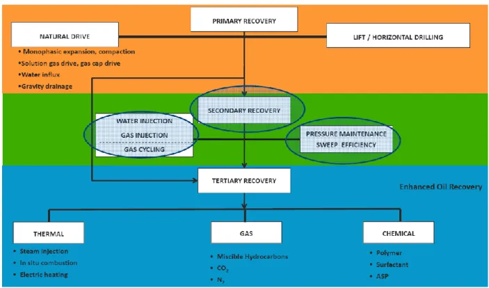
Figure I.1 : reservoir drive mechanisms. ... 3

Figure I.2: Gas/oil displacement results for Berea cores, oil production as a function of time. ... 7

Figure I.3:Buckley-Leverett fractional gas flow plot (based on data from the Hawkins field). ... 10

Figure I.4: Typical Buckley-Leverett saturation profiles. ... 11

Figure I.5 : Effect of viscosity on gas/oil fractional flow. ... 12

Figure I.6 :Cross-sectional view of gas/oil displacement front [at 0.15 pore volumes injected (PVI)] for mobility ratios of (a) 20 and (b) 383 at 0.10 and 0.15 PVI, respectively. ... 14

Figure I.7 : Gas/oil displacements fronts for various mobility ratios (0.151 to 71.5) and PVI until breakthrough, quarter of a five-spot pattern. ... 14

Figure II.1: Location of Menzel Ledjmet Field. ... 19

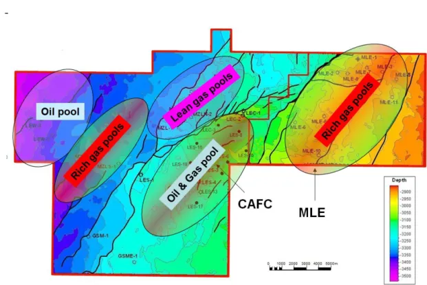
Figure II.2: LES/LEC TAG-I Pool – CAFC & MLE Areas ... 20

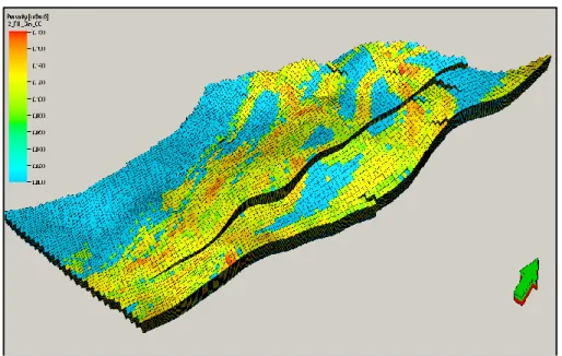
Figure II.3: Porosity distribution(Layer1) ... 24

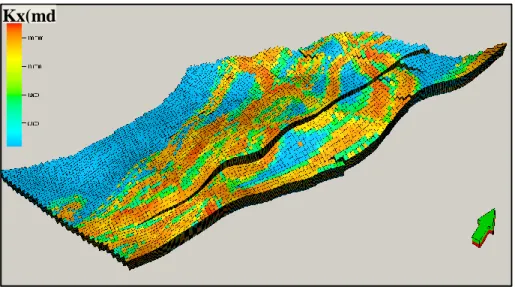
Figure II.4: Permeability distribution (Layer1) ... 25

Figure II.5:Reservoir equilibrium regions ... 28

Figure II.6 : A: 3D view of the section area; B: Cross section showing fluid contacts ... 30

Figure III.1:LES-LEC TAGI Field ... 34

Figure III.2: Daily field production of the sensitivities on Gas Injection ratios ... 36

Figure III.3: Cumulative field production of the sensitivities on Gas Injection ratios ... 37

Figure III.4: Cumulative field Gas production of the sensitivities on Gas Injection ratios ... 37

Figure III.5: Cumulative field Gasinjection of the sensitivities on Gas Injection ratios ... 38

Figure III.6: New well location for the Gas injector (3D View) ... 40

Figure III.7: New well location for the Gas injector (2D View) ... 40

Figure III.8 : Daily Dynamic simulation results for the New Gas injector………..……..…………..41

Figure III.9 : Cumulative dynamic simulation results for the New Gas injector ... 42

Figure III.10: Currentlocation of the Well7 in LES-LEC TAGI...43

Figure III.11 : Results of extension perforations on WELL7...……….……….44

Figure III.12 : Daily Production results of extension perforations on WELL7 vs base case………..…….44

(6)

v

List of tables

Table Page

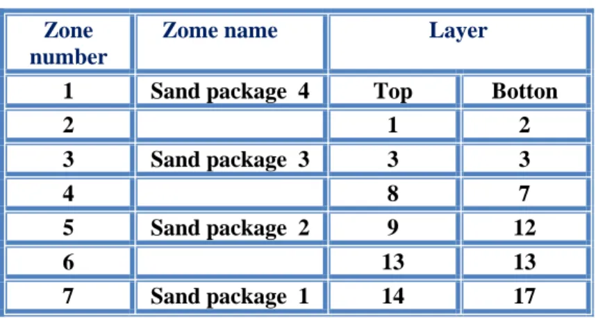
Table II.1: Vertical breakdown and layering ... 22

Table III.1: Sensitivities on Gas injection volumes. ... 39

Table III.2: New Gas injector results vs Base case ... 43

(7)

vi

General

(10)

1

General Introduction

Conventional and unconventional hydrocarbons are likely to remain the main component of the energy mix needed to meet the growing global energy demand in the next 50 years. The worldwide production of crude oil could drop by nearly 40 million B/D by 2020 from existing projects, and an additional 25 million B/D of oil will need to be produced for the supply to keep pace with consumption. Scientific breakthroughs and technological innovations are needed, not only to secure supply of affordable hydrocarbons, but also to minimize the environmental impact of hydrocarbon recovery and utilization.

The lifecycle of an oilfield is typically characterized by three main stages: production buildup, plateau production, and declining production. Sustaining the required production levels over the duration of the lifecycle requires a good understanding of and the ability to control the recovery mechanisms involved. For primary recovery (natural depletion of reservoir pressure), the lifecycle is generally short and the recovery factor does not exceed 20% in most cases. For secondary recovery, relying on either natural or artificial water or gas injection, the incremental recovery ranges from 15 to 25%. Globally, the overall recovery factors for combined primary and secondary recovery range between 35 and 45%.[1]

In our work study the OIL field development plan requested water/gas injection for pressure support and to avoid natural depletion of reservoir pressure.

Water injection process (WIP) is a popular method for Increasing Hydrocarbon Recovery factors and it has been successfully applied in several fields, but in SH-FCP fields there are many reservoirs that Water injection cannot be applied due to its low petro-physical properties, in which makes this process uneconomical to operate. In cases where WIP cannot be applied, gas injection is the most helpful technology for recovering oil in a technical and economically viable.[2]

(11)

Chapter I

(12)

2

I.1.Introduction

Gas injection is certainly one of the oldest methods utilized by engineers to improve recovery, and its use has increased.

Gas injection projects are undertaken when and where there is a readily available supply of gas. This gas supply typically comes from produced solution gas or gas-cap gas, gas produced from a deeper gas-filled reservoir, or gas from a relatively close gas field. Such projects take a variety of forms, including the following:

 Reinjection of produced gas into existing gas caps overlying producing oil columns.

 Injection into oil reservoirs of separated produced gas for pressure maintenance, for gas storage, or as required by government regulations.

 Gas injection to prevent migration of oil into a gas cap because of a natural water drive, down-dip water injection, or both.

 Gas injection to increase recoveries from reservoirs containing volatile, high-shrinkage oils and into gas-cap reservoirs containing retrograde gas condensate.

 Gas injection into very under-saturated oil reservoirs for the purpose of swelling the oil and hence increasing oil recovery.

The primary physical mechanisms that occur as a result of gas injection are:

 Partial or complete maintenance of reservoir pressure  Displacement of oil by gas both horizontally and vertically

 Vaporization of the liquid hydrocarbon components from the oil column and possibly from the gas cap if retrograde condensation has occurred or if the original gas cap contains a relict oil saturation

 Swelling of the oil if the oil at original reservoir conditions was very under-saturated with gas

 Gas injection is particularly effective in high-relief reservoirs where the process is called "gravity drainage" because the vertical/gravity aspects increase the efficiency of the process and enhance recovery of up-dip oil residing above the uppermost oil-zone perforations. [3]

(13)

3

I.2.Drive mechanisms

A reservoir drive mechanism is a source of energy for driving the fluids out through the wellbore. It is not necessarily the energy lifting the fluids to the surface, although in many cases, the same energy is capable of lifting the fluids to the surface.[4]

Figure I.1: reservoir drive mechanisms

I.2.1.Primary recovery mechanisms

 Solution Gas Drive :

This mechanism is mainly observed at the start of Production, expansion of dissolved gases occur, change in fluid volume results in production of reservoir fluids. A solution gas drive reservoir is initially either considered to be saturated or under-saturated. [4]

 Gas Cap Drive :

The decrease in pressure during the production, expansion of Gas cap occur, as production continues, the gas cap expands pushing the gas-oil contact (GOC) downwards.

Better than Solution gas drive .The recovery of gas cap reservoirs is better than for solution drive reservoirs (20% to 40% OOIP).[4]

(14)

4  Water Drive Mechanism:

This is the case of reservoirs bounded by aquifers. During Pressure Depletion, the compressed water expands and over flow towards reservoir. Invading water drive the oil towards producing wells. Water influx acts to mitigate the Pressure Decline. The recovery from water driven reservoirs is usually good (20-60%OOIP).[3]

 Gravity Drainage :

Under density difference effect, the three reservoir fluids (oil, water and gas) segregate creating a secondary energy source. This is relatively a weak mechanism. It can be used as drive mechanism in combination with other drive mechanism

The best conditions for gravity drainage can be in case of thick oil zones or high vertical permeability. Efficiency of gravity drainage is usually low compared to field production rates.[3]

 Combination or Mixed Drive :

In practice, reservoir usually incorporates at least two main drive mechanisms [5]. For example Gas cap & Aquifer are sometimes present together and both free gas and water are in contact with the oil. In such a reservoir some of the energy will come from the expansion of the gas and some from the energy within the massive supporting aquifer and its associated compressibility Sometimes it may be only water drive in the above situations. If the hydrocarbons are taken out at a rate such that for every volume of oil removed water readily moves into replace the oil, then the reservoir is driven completely by water. On the other hand there may be only depletion drive. If the water does not move in to replace the oil, then only the gas cap would expand to provide the drive. [4]

I.2.2.Secondary recovery mechanisms

The natural drainage of oil reservoir often leads to low recovery factors. Additional energy should be injected into oil reservoirs in order to achieve higher recovery. First solution is to inject fluid, water and/or gas, in the reservoir. The objective is supporting pressure and improving the sweeping efficiency of the hydrocarbon zone. [4]

(15)

5

I.2.3 Tertiary recovery

Tertiary recovery or often called enhanced oil recovery includes some advanced methods used at the late life of the reservoir. These techniques usually require deep studies of reservoir fluid and rock and also high investment costs. Among the EOR techniques there are thermal processes, chemical processes and miscible gas injection. [4]

I.3.Gas injection mechanism

The decision to apply gas injection is based on a combination of technical and economic factors. Deferral of gas sales is a significant economic deterrent for many potential gas injection projects if an outlet for immediate gas sales is available. Nevertheless, a variety of opportunities still exist. First are those reservoirs with characteristics and conditions particularly conducive to gas/oil gravity drainage and where attendant high oil recoveries are possible. [6] Second are those reservoirs where decreased depletion time resulting from lower reservoir oil viscosity and gas saturation in the vicinity of producing wells is more attractive economically than alternative recovery methods that have higher ultimate recovery potential but at higher costs. And third are reservoirs where recovery considerations are augmented by gas storage considerations and hence gas sales may be delayed for several years.

The purposes of this section include listing the physical criteria that separate the successful gas injection operations from the unsuccessful ones, describing the reservoir and process variables that must be defined and quantified, and demonstrating some of the simple techniques available for predicting and evaluating field performance. Some of these calculations can be performed with spreadsheets or, more tediously, with hand-held calculators. Modern numerical reservoir simulators are commonly used to calculate the projected performance of applying immiscible gas injection to a particular reservoir. For reservoirs with several years of immiscible gas injection, these same simulators can be used to history match past performance and to project future performance under various scenarios (e.g., continuing current operations, evaluating various new producing wells options, or comparing surface facility operational alternatives). [7]

Specifically not included in this chapter is any discussion of the factors to consider in implementing a gas injection project, such as gas compression needs, gas distribution systems,

(16)

6

wellbore configurations, and vessel selection and sizing for handling produced fluids. These subjects are covered in various chapters in the Production Operations Engineering and Facilities and Construction Engineering sections of the Handbook. [7]

I.3.1. Microscopic and Macroscopic Displacement Efficiency of Gas Displacement

The conceptual aspects of the displacement of oil by gas in reservoir rocks are discussed in this section. There are three aspects to this displacement: gas and oil viscosities, gas/oil capillary pressure (Pc) and relative permeability (kr) data, and the compositional interaction, or component mass transfer, between the oil and gas phases. The first two topics are discussed in this section; the third is discussed in the next section.[7]

I.3.2.Gas/Oil Viscosity and Density Contrast

One must first understand the viscosity and density differences between gas and oil to appreciate why the gas/oil displacement process can be very inefficient. Gases at reservoir conditions have viscosities of ≈0.02 cp, whereas oil viscosities generally range from 0.5 cp to tens of centipoises. Gases at reservoir conditions have densities generally one-third or less than that of oil. Thus, gas is generally one to two orders of magnitude less viscous than the oil it is trying to displace. Regarding the fluid density difference, gas is always considerably "lighter" than the oil; hence, gas, when flowing, will segregate by gravity to the top of the reservoir or zone and oil will "sink" simultaneously to the bottom of the reservoir or zone.

Another gas/oil property that must be known for calculations at reservoir conditions is the interfacial tension (IFT) between the oil and gas fluid pair. This value is needed at reservoir conditions for the conversion of gas/oil capillary pressure data from surface to reservoir conditions. A number of technical papers discuss the calculation of IFT from compositional information about the oil and gas phases [8] [9]. As the pressure increases, the IFT values decrease, although not low enough for miscible displacement to occur. Although not illustrated in the table, it should be noted that the IFT between nitrogen and oil is higher than that between a lean natural gas and the same oil. [10]

(17)

7

I.3.3.Gas/Oil Capillary Pressure and Relative Permeability

The gas/oil capillary pressure and relative permeability data are typically measured by commercial laboratories using routine special core analysis procedures. Gas-oil capillary pressure data can be measured with either porous-plate or centrifuge equipment. One approach for obtaining gas/oil relative permeability data is the viscous displacement method in which gas displaces oil. A second method is the centrifuge method, which is generally used to obtain capillary pressure and relative permeability information simultaneously.

In all cases, gas is the non-wetting phase in this displacement; hence, it will preferentially flow through the largest pores first. However, what is very important in the determination of the oil relative permeability is the distribution of the oil phase in the core sample because in real reservoirs connate water occupies the smallest pores. As shown by Hagoort, [11] initial water saturation has a significant effect on oil relative permeability during the gas/oil displacement (centrifuge experiments). The water phase will occupy a greater percentage of the smaller pore spaces as the connate water saturation increases. As a result, the pore structure appears more streamlined to the oil and gas phases. The oil relative permeability at higher connate water saturations is considerably higher ( Figure I.2 ).

(18)

8

This figure shows that long drainage times are required for displacement of oil to low saturation values.

The other key aspect of the oil relative permeability (kro) is the determination of its value as the oil saturation decreases. Because oil relative permeability becomes quite low but nonzero, the time to reach equilibrium in laboratory core plug measurements can be very long. Figure I.2 presents experimental results for cumulative oil recovery as a function of drainage time and shows that the oil continues to flow but more and more slowly (linearly as a function of the logarithm of tD).

If the gas/oil relative permeability data were measured with the viscous displacement technique (the extended Welge technique as described by Johnston et al.) [12],extra care is needed in applying these data. First, the displacement of oil by gas is at an unfavorable mobility ratio (see discussion below) that makes the process unstable. Second, a displacement is adversely affected by capillary end effects that, for the gas/oil system, cannot be overcome by high gas throughput rates. At low oil saturations, the region of most interest, the capillary end effect is the greatest.[11]

Finally, one method developed to affect the gas/oil relative permeability and to reduce gas mobility is to inject water alternately with gas (WAG). This procedure was proposed by Caudle and Dyes[13].Although the method was proposed for use in miscible gas floods, the concept applies equally to immiscible gas displacements. This technique has been used in many west Texas CO2 miscible gas projects, in the Prudhoe Bay miscible flood[14] , and in the Kuparuk immiscible and miscible gas injection processes.[15]

The three-phase gas, oil, and water relative permeabilities are calculated in numerical reservoir simulators with algorithms developed over the past several decades. [16]

I.3.4.Mobility Ratio

The mobility of a fluid (Eq. I.1) is defined as its relative permeability divided by its viscosity. Mobility combines a rock property, permeability, with a fluid property, fluid viscosity. Gas-oil relative permeabilities are assumed to be dependent on the saturations of the two fluid phases and independent of fluid viscosity:

(19)

9

A fluid’s mobility relates to its flow resistance in a reservoir rock at a given saturation of that fluid. Because viscosity is in the denominator of this definition, gases, which are very-

low-viscosity fluids, have very high mobility.[12]

M =

kg @sorg μo

ko @swiμg

(I.2)

Mobility ratio is generally defined as the mobility of the displacing phase (in the gas/oil case, gas) divided by the mobility of the displaced phase, which is oil. It can also be written in more familiar engineering terms as the ratio of the two fluids’ relative permeability values multiplied by the ratio of the two fluids’ viscosities.

𝑀 =

krg

k_ro

μ_o

μ_g

(I.3)

For simple calculations, the mobility ratio is calculated at the endpoint relative permeability values for the two phases.

All displacements of oil by gas are at "unfavorable" mobility ratios, with typical values of 10 to 100 or more.[17]

I.3.5.Gas/Oil Linear Displacement Efficiency

The equations that characterize the mechanics of oil displacement by an immiscible fluid were developed by Buckley and Leveret [18] using relative permeability concepts and Darcy’s law describing steady-state fluid flow through porous media. The resulting fractional flow equation describes quantitatively the fraction of displacing fluid flowing in terms of the physical characteristics of a unit element of porous media. Assumptions inherent in their work are steady-state flow, constant pressure, no compositional effects, no production of fluids behind the gas front, no capillary effects, movement of advancing gas parallel to the bedding plane, immobile water saturation, and uniform cross-sectional flow (no gravity segregation of fluids within the element). Subsequent work by Welge [19] made solving the displacement equations easier.

(20)

10 is calculated as

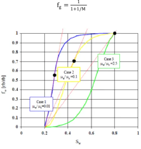
When gravity is negligible, the Welge equation for the fractional flow of gas at any gas saturation (Sg) isexpressedin more familiar Buckley-Leverettequation:

f

_g

=

1

1+1/M

(I.4)

Figure I.3:Buckley-Leverett fractional gas flow plot (based on data from the Hawkins field).

To relate the fraction of gas flowing to time, Buckley and Leverett developed the following material-balance equation:

𝐿 = qtt

∅A

dfg

dsg (I.5)

The value of the derivative dfg/dSg may be obtained for any value of gas saturation by determining slopes at various points on the fg vs. Sg curve. These slopes can be determined manually or, more precisely, using the method presented by Kern [20] for computer spreadsheets. Figure I.4 illustrates calculated gas-saturation distributions derived from the no-gravity and with-no-gravity fractional flow curves shown in (Figure I.3). The area beneath each

(21)

11

curve represents the gas-invaded zone. The saturation profile calculation results in lengths that first increase as saturation decreases and then decrease at lower saturations. While correct from a material-balance standpoint, it has been customary to square off the leading edge of the curve at the breakthrough saturation to account for capillary pressure that was neglected in the original derivation of the equation.

FigureI.4: Typical Buckley-Leverett saturation profiles.

The gas/oil displacement efficiency, the percent of the oil volume that has been recovered, can be calculated for any period of gas injection by integrating the volume of the gas-invaded zone as a function of gas saturation (Sg). Hence, the fractional flow curves (Figure I.4) are used to generate saturation profiles (Figure I.4) that lead to values for the gas/oil displacement efficiency. In the next section, several of the factors affecting this efficiency are discussed.[21]

I.3.6.Factors Affecting Gas/Oil Displacement Efficiency

The fractional-flow and material-balance equations discussed above are important for understanding the effects on the efficiency of the gas/oil displacement process of (1) initial saturation conditions, (2) fluid viscosity ratios, (3) relative permeability ratios, (4) formation dip, (5) capillary pressure, and (6) factors of permeability, density difference, rate of injection, and cross section open to flow. [21]

(22)

12

 Initial Saturation Conditions: If gas injection is initiated after reservoir pressure has declined below the bubble point, the gas saturation will decrease the amount of displaceable oil. If the free gas saturation exceeds the breakthrough saturation, no oil bank will be formed. Instead, oil production will be accompanied by immediate and continually increasing gas production. Laboratory investigations and mathematical analyses have demonstrated this influence of gas saturation on gas displacement performance [22]. Swi has been shown to have no influence on displacement efficiency at gas breakthrough, but it directly affects the displaceable oil volume[23]. If Swi is mobile, the displacement equations are not directly applicable because they were developed for two-phase flow. Approximations of gas displacement performance can usually be made when three phases are mobile by treating the water and oil phases as a single liquid phase. Displacement calculations can then be made with krg and kro data determined from core samples containing immobile water saturation. Oil recovery can be differentiated from total liquid recovery on the basis of material balance calculations incorporating estimated minimum interstitial water saturation.

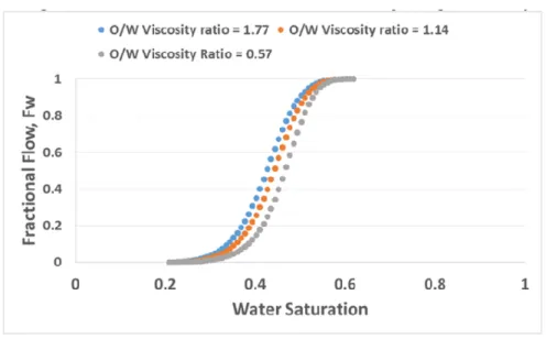
 Fluid Viscosities. The effect of oil viscosity on fractional flow is illustrated in Figure I.5 In this plot, the Sg at breakthrough increases from 12 to 38% with a 10-fold decrease in oil viscosity.[21]

(23)

13

 Relative Permeability Ratios: The concepts of relative permeability can be applied equally well to complete or partial pressure-maintenance operations. Relative permeability, a characteristic of the reservoir rock, is a function of fluid saturation conditions. It is important that calculations be based on dependable data obtained by laboratory analyses at reservoir conditions using representative core samples. If possible, the laboratory-determined data should be supplemented by relative permeabilities calculated from field performance data.

 Formation Dip. When formation dip aids gravity, as illustrated in Figure I.4, fractional flow behavior is significantly improved if permeability is high enough and withdrawal rates do not exceed gravity-stable conditions. Gravity drainage is discussed later in this chapter.[21]

 Capillary Pressure. Capillary forces are opposite gravity drainage forces and directionally decrease displacement efficiency. However, capillary forces can often be ignored as insignificant for projects with rates of displacement normally used. Only at extremely low rates of displacement, where viscous forces become negligible, is the saturation distribution controlled to a significant extent by the balance between capillary and gravitational forces. Another place where capillary forces are considered important is many of the large carbonate reservoirs of the Middle East where the matrix-blocks/fracture-system interaction can significantly affect overall reservoir performance.

 Other Factors. Higher permeability, greater density difference between oil and gas, and a lower displacement rate all improve the displacement efficiency.[21]

I.3.7.Unfavorable Mobility Ratio Causes Viscous Flow Instabilities

Displacements that take place at very unfavorable mobility ratios are unstable, and viscous fingering occurs. This is the situation for essentially all gas/oil displacements, especially if the displacement is occurring horizontally. The impact of such instabilities is illustrated in Figures. I.6 and I.7. [24] [25] Both figures were drawn from technical literature concerning miscible displacement laboratory experiments using homogeneous sandpacks, but the observed effects would be the same for immiscible gas displacing oil at very unfavorable mobility ratios. Figure I.6 shows, in cross-sectional view, the nature of viscous fingering for two highly unfavorable mobility ratios (the two fluids have equal densities). The flood front in both cases is very

(24)

14

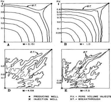
unstable. Figure I.7 shows, in areal view, the effect of mobility ratio on the displacement process in a quarter of a five-spot pattern for mobility ratios from 0.151 to 71.5. For mobility ratios from 4.58 to 71.5 (cases D through F), the flood front is very unstable, and breakthrough occurs via narrow fingers of the injected fluid; these cases show how the process of gas displacing oil would occur.[21]

Figure I.6 :Cross-sectional view of gas/oil displacement front [at 0.15 pore volumes injected (PVI)] for mobility ratios of (a) 20 and (b) 383 at 0.10 and 0.15 PVI, respectively. [24]

Figure I.7 : Gas/oil displacements fronts for various mobility ratios (0.151 to 71.5) and PVI until breakthrough, quarter of a five-spot pattern. [25]

(25)

15

In both of these illustrations, the cause of the viscous fingering was a slight perturbation in the flow field that grew into the viscous finger once the perturbation occurred. In real reservoir situations, there are two physical aspects that enhance the viscous-fingering phenomenon. First, real reservoirs are very heterogeneous, so a variety of styles of permeability heterogeneities can initiate viscous fingering. Second, in a cross-section immiscible gas/oil displacement process, gas is always less dense than oil. Hence, there is a gas/oil density difference, and the force of gravity causes the gas to override the oil and initiate a viscous finger of the high-mobility gas phase along the top of the reservoir interval.

If the gas/oil displacement is occurring vertically with gas generally displacing oil downward, gravity will work to stabilize the flood front between the gas and oil, although if the rate is too high, instabilities in the form of gas cones or tongues can occur.[21]

I.4. General Immiscible Gas/Oil Displacement Techniques

I.4.1. Types of Gas-Injection Operations

Immiscible gas injection is usually classified as either crestal or pattern, depending on the location of the gas injection wells. The same physical principles of oil displacement apply to either type of operation; however, the overall objectives, type of field selected, and analytical procedures for predicting reservoir performance vary considerably by gas injection method.[26]

 Crestal Gas Injection: sometimes called external or gas-cap injection, uses injection wells in higher structural positions, usually in the primary or secondary gas cap. This manner of injection is generally used in reservoirs with significant structural relief or thick oil columns with good vertical permeability. Injection wells are positioned to provide good areal distribution and to obtain maximum benefit of gravity drainage. The number of injection wells required for a specific reservoir depends on the injectivity of individual wells and the distribution needed to maximize the volume of the oil column contacted.

Crestal injection, when applicable, is superior to pattern injection because of the benefits of gravity drainage. In addition, crestal injection, if conducted at gravity-stable rates—e.g., less than the critical rate will result in greater volumetric sweep efficiency than pattern injection

(26)

16

operations. There are many examples of ongoing crestal injection projects throughout the world, including some very large projects in the Middle East.[26]

 Pattern Gas Injection: sometimes called dispersed or internal gas injection, consists of a geometric arrangement of injection wells for the purpose of uniformly distributing the injected gas throughout the oil-productive portions of the reservoir. In practice, injection-well/production-well arrays often vary from the conventional regular pattern configurations—e.g., five-spot, seven-spot, nine-spot (see the chapter on waterflooding in this section for more description of these patterns)—to irregular injection-well spacing. The selection of an injection arrangement is a function of reservoir structure, sand continuity, permeability and porosity levels and variations, and the number and relative locations of existing wells.[26]

This method of injection has been applied to reservoirs having low structural relief, relatively homogeneous reservoirs with low permeabilities, and reservoirs with low vertical permeability. Many early immiscible gas-injection projects were of this type. The greater injection-well density results in pattern gas injection, rapid pressure and production response, and shortened reservoir depletion times.

There are several limitations to pattern-type gas injection. Little or no improvement in recovery is derived from structural position or gravity drainage because both injection and production wells are located in all areas of the reservoir. Low areal sweep efficiency results from gas override in thin stringers and by viscous fingering of gas caused by high flow velocities and adverse mobility ratios. High injection-well density increases installation and operating costs. Typical results of applying pattern injection in low-dip reservoirs are rapid gas breakthrough, high producing GORs, significant gas compression costs to reinject the gas into the reservoir, and an improved recovery of < 10% of original oil in place (OOIP). Note that gas inefficiently displaces oil in gas-swept areas. Attempts to subsequently waterflood such areas result in rapid water breakthrough and little, if any, additional oil displacement.

Few pattern gas injection projects have been implemented in recent years because this method is not as attractive economically as alternative methods for increasing oil recovery.[26]

(27)

17

I.4.2.Optimum Time To Initiate Gas Injection Operations

The optimum time to begin gas injection is site specific and depends on a balance of risks, gas market availability, environmental considerations, and other factors that affect project economics. When only oil recovery and improvements in reservoir producing characterstics are considered, reservoir conditions for gas injection operations are usually more favorable when the reservoir is at or slightly below the oil bubble point pressure, unless the bubble point pressure is low compared with the initial reservoir pressure. Near the oil bubble point pressure, non- recovered oil represents the smallest volume of stock-tank oil, oil relative permeability is high, and oil viscosity is low.[27]

I.4.3.Efficiencies of Oil Recovery by Immiscible Gas Displacement

It is customary in most displacement processes to relate recovery efficiency to displacement efficiency and volumetric sweep efficiency. The product of these factors provides an estimate of recoverable oil expressed as a percentage of OOIP. Analytical procedures are available for evaluating each efficiency factor. For the purposes of this chapter, the two components describing the overall recovery efficiency are defined as follows:

1. Displacement efficiency is the percentage of oil in place within a totally swept reservoir rock volume that is recovered as a result of viscous displacement and gravity drainage processes.

2. Volumetric sweep efficiency is the percentage of the total rock or PV that is swept by gas. This factor is sometimes divided into horizontal and vertical components, with the product of the two components representing the volumetric sweep.

Recovery efficiencies increase with continued gas injection, but the rate of recovery diminishes after gas breakthrough occurs as the GOR increases. The overall result is that the ultimate oil recovery efficiency is a function of economic considerations, such as the cost of gas compression and the volume and availability of lean residue gas or potentially more expensive alternatives like N2 from a nitrogen rejection plant.[27]

(28)

18

I.5.conclusion

Gas injection is one of the methods utilized by engineers to improve recovery, and its use has increased.

Gas injection mechanisms that occur as a result of gas injection are:  Partial or complete maintenance of reservoir pressure

 Displacement of oil by gas both horizontally and vertically

 Vaporization of the liquid hydrocarbon components from the oil column and possibly from the gas cap if retrograde condensation has occurred or if the original gas cap contains a relict oil saturation

 Swelling of the oil if the oil at original reservoir conditions was very undersaturated with gas

 Gas injection is particularly effective in high-relief reservoirs where the process is called "gravity drainage" because the vertical/gravity aspects increase the efficiency of the process and enhance recovery of up-dip oil residing above the uppermost oil-zone perforations.[28]

(29)

CHAPTER II

(30)

19

II .1.Introduction

The Menzel Ledjmet East (MLE) natural gas and liquids project under taken by ENI and Sonatrach on Block 405 b in the Berkine basin has been brought into production just in 2013. The MLE project, which entailed the development of the MLE wet gas field that has just comeon stream and the Central Area Field Complex (CAFC) oil and gas field, has an important production capacity.[2]

II.2.Geographic location

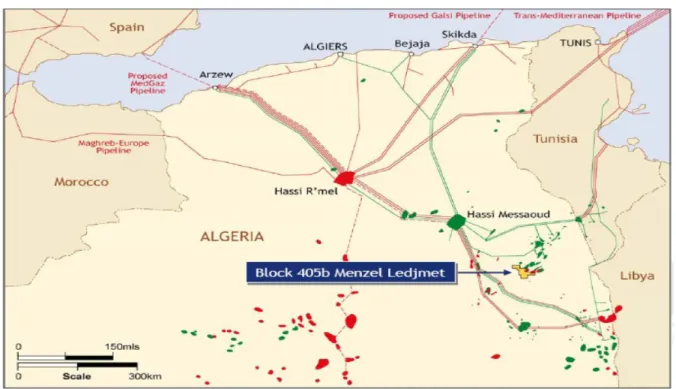
The Menzel Ledjmet Block 405b is located in the Berkine Basin in the desert region of Algeria.It is about220km southeast of Hassi Messaoud (Ouargla). That's 1,000 km southeast of Algiers. The exploitation contract was signed between SONATRACH and the Canadian company FCP than the Italian company ENI replaced FCP.

Figure II.1: Location of Menzel Ledjmet Field.

The field contains numerous hydrocarbon accumulations that can be commercially exploited to the benefit of the Algerian State, SONATRACH and ENI. They consist of oil, lean gas and rich gas pools. The west area of block 405b, Central Area Complex Field (CAFC), where this

(31)

20

study was carried out, is developed in synergy with the East part called MLE. The CAFC is located to the west of the MLE field. [2]

CAFC is characterized by different Reservoirs and Single Well Pools (SWP) mineralized with Lean Gas, Rich Gas and Oil as summarized below:

- TAGI Oil reservoir (The multi-well LES/LEC TAGI Sequence 3 oil pool and gas cap).

- F6-2 Lean gas reservoir. - F6-2 Rich gas reservoir.

- F6-2 SWP lean and rich gas pools. - F6-2 SWP oil.

- F6-1 Light oil reservoir. -

(32)

21

II.3. Static model

The LES/LEC TAG-I pool contains a volatile oil with an overlying rich gas cap. Bottom water has been penetrated by 3 wells within the pool. At the beginning, a 3-D dynamic reservoir simulation model was constructed using Computer Modeling Group’s GEM equation of state simulation software. This model was conditioned to honor the well tests and lab data and used to help plan development of the reservoir and to evaluate the oil and gas recovery potential for various development options. Later, this model had been reconstructed using ECLIPSE simulation software; it has the following primary building blocks:

 The Petrel geological model modified in a geologically reasonable fashion to replicate well and interference test behavior.

 A model of the reservoir oil that reasonably replicates the phase behavior measured in the laboratory and in well tests.

 Rock-fluid interaction parameters that reflect the identified facies associations and special core analysis data.

 Vertical flow models for the production and injection wells that were tuned to match well test data. [29]

II.3.1. Geocellular model

The model combined various inputs from multiple sources. Geophysical data was used to create the structure for the geocellular grid, while petrophysical data was used to populate the grid cells. The geocellular model consists of 8 horizons with layers of varying thicknesses. The grid cells have an aerial resolution of 100m*100m, the same as the simulation grid. Vertically, the grid contains 7 zones, based on the flow units within the TAG-I (Seq-3) which is collectively separated into 17 proportional thickness layers. [30]

(33)

22

Table II.1: Vertical breakdown and layering Zone

number

Zome name Layer

1 Sand package 4 Top Botton

2 1 2 3 Sand package 3 3 3 4 8 7 5 Sand package 2 9 12 6 13 13 7 Sand package 1 14 17

II.3.2. Geological model

The TAG-I Sequence 3 was treated as a series of braided fluvial systems intermingled with meandering channels. These braided systems have been identified in the core as 4 separate units within the TAG-I Sequence 3. The 4 flow units are separated by either complete barriers or partial barriers depending upon were they are stratigraphically, which were identified on logs as well as in cores. [30]

II.3.3.Structural Framework

The structural framework was created in Petrel, and covers the entire Ledjmet Block 405b. The structural model was based on seismic fault interpretations and seismic time horizons. A total of 3 seismic time horizons (Senonian Salt, Liassic Salt, and TAG-I) were used to generate the TAG-I Sequence 3 depth structure which was used in the geocellular model. The time surfaces were depth converted using interval velocities. The depth structures were tied to the well tops after each interval velocity function was applied. It was assumed the TAG-I reflector represented the top of the TAG-I Sequence3.

The fault framework was generated in pillar gridding process‟ using directional faults polygons, boundary segments and trends in order to keep the grid as orthogonal as possible and lined up at about 30° deg azimuth which is the predominant direction of deposition. [30]

(34)

23

II.3.4. Petrophysical inputs

A total of 4 petrophysical properties were distributed; Facies, Effective Porosity, horizontal permeability and water saturation. The well log data was normalized and calibrated with core data before it was used in the geocellular model. Porosity and permeability were the two main parameters used, as they were the basis for both the facies calculation and capillary pressure calculations. The discrete facies property was based on the calculated FZI, which incorporates core, MREX, and wireline log inputs. Both effective porosity and permeability were calibrated with all available core data, and analyzed across Ledjmet Block 405b to ensure all relevant petrophysical data were captured in the geocellular modeling. [31]

a. Flow Facies and Flow Units

The different flow zones defined from petrophysical data were classified into four representative types of facies:

- Channel high energy - Channel high energy - Levee

- Shale

b. Porosity

The porosity of porous media is defined as the ratio of the volume of the pores to the total bulk volume of the media (usually expressed as fraction or percent).[32] Let us select any Point of the porous media and its environment with a sufficiently large volumeV𝑇 , where:

V_𝑇 = v_p + v_s (II.1)

Porosity is defined as the ratio of pore volume to total volume, which can be expressed as:

∅ = Vp

VT =

vT−vs

VT (II.2)

Much like the facies modeling, all available data was used to model the effective porosity (PHIE). The PHIE was upscaled, biased to the facies, into the grid resolution using arithmetic

(35)

24

averaging. Data analysis was performed on a facies by facies basis, therefore all the data conditioning and trends are applied to the PHIE for each flow facies per flow zone. A vertical variogram was created and used for the porosity of each facies. The PHIE was distributed throughout the geocellular model based on the facies model. [31]

Figure II.3: Porosity distribution(Layer1)

c. Permeability:

Permeability in a reservoir rock is associated with its capacity to transport fluids through a system of interconnected pores, i.e. communication of interstices. In general terms, the permeability is a tensor, since the resistance towards fluid flow will vary, depending on the flow direction. In practical terms, however, [33] permeability is often considered to be a scalar, even though this is only correct for isotropic porous media.

If there were no interconnected pores, the rock would be impermeable, i.e., it is natural to assume that there exists certain correlations between permeability and effective porosity.

Similar to the previously discussed reservoir property models, the horizontal permeability was distributed stochastically. Porosity / Permeability cross plots were created and imposed in the modeling. Both the facies and porosity models were the basis for the permeability model. [12]

(36)

25

Figure II.4: Permeability distribution (Layer1)

d. Water saturation:

The equilibrium fluid saturation distribution in a petroleum reservoir, prior to production is governed by the pore space characteristics. This is as a result of the non-wetting phase, normally hydrocarbons, entering pore space initially occupied by the wetting fluid, normally water, [34] during migration of hydrocarbons from a source rock region into a reservoir trap. A pressure differential is required for the non-wetting phase to displace wetting phase and this is equivalent to a minimum threshold capillary pressure and is dependent on pore size.

Water saturation was the only property not modeled on well log responses. Instead of using up scaled water saturation (Sw) curves, saturation height functions were used to create the Sw model.

To apply the saturation height functions, a height above contact property was generated using an ―Oil Down To‖ contact at 3135m subsea. [31]

Kx(md )

(37)

26

II.4. Dynamic model

The reservoir was simulated using a compositional simulator.

II.4.1. Short Overview on ECLIPSE software for numerical Simulation

ECLIPSE is a batch program. The engineer creates a single input data file for ECLIPSE. This data file contains a complete description of the model. The *.DATA file, commonly called a ―data file‖ or ―data deck,‖ is subdivided into sections: RUNSPEC, GRID, EDIT, PROPS, REGIONS, SOLUTION, SUMMARY, SCHEDULE. Within these sections, you can use keywords to identify input data, request output data, and specify conditions.

ECLIPSE reads the input data file section by section and processes each section in turn once that section has been read. Various data and consistency checks are made before proceeding to the next section. [14]

The last section is exceptional because it specifies time-dependent data and is not read and processed as a whole; the keywords are processed in the order they are read from the data file. The first task performed by ECLIPSE is to allocate memory for the input data (RUNSPEC section). Although ECLIPSE is dynamically dimensioned and reserves s much memory as required for the simulation as a whole, different kinds of information in the simulation require varying amounts of memory.

The simulation grid geometry and properties are processed into a form more convenient for calculation of flows. For each cell, ECLIPSE calculates the pore volume, transmissibility in three dimensions and cell center depth and creates connections to other cells to/from which fluids may flow (GRID section).

These quantities may be modified either by the user or by ECLIPSE (EDIT section).

The rock fluid properties are specified next. The term fluid properties refer to a set of input tables that effectively define the phase behavior of each flowing phase. The term rock properties refer to sets of input tables of relative permeability and capillary pressure versus saturation. Effectively, this defines the connate, critical and maximum saturation of each phase, supplies information for defining the transition zone and defines the conditions of flow of phases relative to one another. This strongly affects the ratios of produced phases that are water cuts and GORs (PROPS section).

(38)

27

Next, the initial conditions are defined, often by specifying the OWC and/or GOC depths and the pressure at a known depth. ECLIPSE uses this information in conjunction with much of the information from previous stages to calculate the initial hydrostatic pressure gradients in each zone of the reservoir and allocate the initial saturation of each phase in every grid cell prior to production and injection. This is called initialization (SOLUTION section). [35]

The final section of the data file is where simulation actually begins. Wells are drilled, perforated and completed, production and injection targets are set up, wells are opened and fluids flow through the reservoir, driven by the wells (SCHEDULE section). [35]

ECLIPSE outputs a variety of information on the simulation results and its progress at dates during the simulation defined by the user (SUMMARY section).

When the run has finished, the output is examined using text editors and post-processors of various degrees of sophistication. [35]

II.4.2. Properties distribution from geocellular model

- Simulation grid: The model has grid dimensions 59*141*23. A corner point gridding was used. Each cell has 100*100m area and a variable thickness.

- Permeability and porosity: The geological parameters distribution was taken from the static model described above.

- NET to GROSS: initially all the cells were supposed to be filled 100% of fluids. [36]

II.4.3. Wells:

At the beginning of the LES/LEC TAGI reservoir study, 5 explorationvertical wells were drilled. From PVT analysis, 3 wells were identified as oil wells (OP3, OP6, and OP8); the remaining 2 were gas condensate (GI2, GI7). After that, 7developmentwells were drilled: (OPc3, OP10, OPH11,OPH19, OPH20, OPH21, OPH22). [36]

(39)

28

II.4.4. Rock-Fluid Interaction

A total of 12 saturation functions were generated from laboratory experiments: 6 for imbibition and 6 for drainage. The HYSTERISIS keyword of ECLIPSE was used to handle both series of curves for each cell. The distribution of the 12 functions on the grid cells was done using the SATNUM and IMBNUM of ECLIPSE.

Each saturation function contains 4 tables defining:  Oil water relative permeability curve.  Oil gas relative permeability curve.  Oil water capillary pressure curve.  Oil gas capillary pressure curve.

II.5. Rock compaction

From laboratory studies, the rock compaction was assumed 6.5267E-05bar-1 at a reference depth of 361.51 bar. [36]

II.5.1.Fluid contacts

The LES/LEC TAGI reservoir is composed of two equilibrium regions representing the main area and the east one.

(40)

29 - Main area:

 Gas-Oil Contact is defined at 3107m for both regions.

 Oil-Water Contact: From RCI data, the oil water contact is defined at 3135 for the main area and 3122m for the east one.

- East area: this area contains gas condensate, a gas water contact is defined at 3122 mSSTVD

II.5.2.Fluid model

Due to fluid type difference between east and main area, 2 different fluid models were defined. Both equations of state are 12-pseudo-component Peng-Robinson Equation of State (―EOS‖). The equations of state were tuned to reasonably various laboratory measurements of the selected reservoir oil (from OP3) and gas (OP10), including:

 Single- and multi-stage separator tests.  Differential liberation data.

 Slim tube test behavior.  Constant Mass Expansion.

(41)

30

Figure II.6 : A: 3D view of the section area; B: Cross section showing fluid contacts

II.6. Field development plan

The initial development of this field will be on a maximum of 30 years divided on two periods:  The first 10 years:

 Full pressure maintain by Water and associated gas re-injection. The related oil production plateau IS 2500 M3/D. The produced gas will be re-injected into the gas cap at peak rates of 120 MMscf/d.

 Oil displacement by water was supposed to be a stable process in this reservoir because of a favorable mobility ratio. Expected water injection rate was 500 to 720 m3 to

W

E

W

E

A

(42)

31

maintain reservoir pressure, and this was facilitated by drilling a total of 3 water injectors in the field.

 Water produced from the Barremian will be injected also into the reservoir’s water leg for pressure maintain.

 Blowdown phase: Injection will be stopped and gas injectors will be transformed into producers.

To optimize the the development of LES/LEC TAGI, a total of 16 wells are drilled. Five exploration and appraisal wells have penetrated this reservoir between. Two pressure interference tests were conducted between the five existing wells to confirm reservoir continuity between these wells. With the two successful pressure interference tests conducted in the central portion of the LES/LEC TAGI pool, reservoir continuity between the five existing wells (OP3, OP6, GI7, OP8, and GI2) has been proven. [37]

II.6.1.Development wells

LES/LEC TAGI Pool developed with an optimized pressure maintenance scheme with water injection, solution gas re-injection and optimized blow down of the gas cap to have a commercial gas sales profile when combined with MLE. The current development involves a total of 15 wells of which:

 8 oil producers (4 Horizontals, 1 Deviated and 3 verticals)

 1 gas producer (vertical)

 3 gas injectors

 3 water injectors

In addition to the previous development wells, 3 source water wells had been already drilled. A horizontal well (OP26) has been drilled on the east area with negative results (water bearing). After the results of this well and also the results ofOP10 (gas condensate instead of oil) the development of the east area is postponed. Two planned wells in this area (one injector and one producer) are put on hold. [37]

(43)

32

II.7. Conclusion

At the end of this chapter, we can say that the LES/LEC TAGI reservoir model gathers the majority of the real field available data. It is quite worth to use this dynamic model in order to translate considerably the field behavior. The heterogeneity and the complexity of the Menzel Ledjmet reservoir needs more and more studies and interpretations.

The geological uncertainties are so important in the reservoir model and should be considered in any future work in the purpose of better enhancing the target to «The Model reflects the real field behavior».

(44)

Chapter III

(45)

33

III.1. Introduction on Field development plan

The initial development of LES-LEC TAGI will be on a maximum of 30 years divided on two periods:

 The first 10 years: Injection phase:

 First Production: December 1st, 2016 for early production scenario, with water injection and starting from August 1st, 2017 start-up the total re-injected of produced gas into the gas cap to achieve full pressure maintenance.

 Production plateau: target oil rate = 2500 Sm3/d (~15700 bbl/d), maximum gas rate= 3.4 MSm3/d (~ 120 MMscft/d). In the early production case the start-up rate has been assumed equals to 8000 bbl/d.

 Maximum drawdown for oil producers 500 psi

 Maximum drawdown for gas producers 400 psi

 Downtime = 5%

 Well constrain: Minimum THP = 80 bar. [20]

 After 10 years: Blow-down phase:

Injection will be stopped and gas injectors will be transformed into producers to have a commercial gas sales profile when combined with MLE.

 Target gas production rate = 5.7 Msm3/d (~ 200MMscf/d)

 Well constrain: Minimum THP = 35 bar (gas production diverted to MLE CPF). Development wells:

The current development involves a total of 19 wells of which:

 12 oil producers.

 4 gas injectors.

(46)

34

III.2. Proposed Development Plan Optimization description

The CAFC oil project is mainly composed of two fields: LES-LEC TAGI (TAGI Seq-3) and LEW-Area (Lower Devonian F6-2). The development plan of LES-LEC TAGI required a full water/gas injection for pressure support. In the other side, LEW- area will be developed in natural depletion. [37]

As per POD (plan of development), three water injectors were drilled on LES-LEC TAGI reservoir with a target rate of 18000 Rbbl/d in order to support the reservoir pressure and maximize recovery.

Unfortunately, the three wells have crossed the reservoir on a very poor area with low petro physical properties. Many attempts have been realized in order to sustain the water injection process, the three wells have been stimulated with hydraulic fracturing and acidizing but with negative results, the wells injectivity remains very low confirming a limited connectivity to the production area. [37]

With the production start-up of CAFC Oil project on Dec 2016, the LES/LEC TAGI wells have shown very lower performance than expected.

(47)

35

In addition to that, a horizontal well has been drilled on the east area of the reservoir with totally negative results (found water bearing). Based on that, the drilling of a second well in the east lobe was postponed till the better understanding of the reservoir compartmentalization.

With all these constraints, it was impossible to reach a stable production plateau as expected on the POD. [37]

 Proposed solutions:

In this chapter, we will give some proposals to mitigate the production depletion of CAFC oil wells. Each proposal will be presented by a simulation scenario predicting the reservoir behavior and using a proper Reservoir dynamic modeling simulator (Schlumberger Eclipse Software).

The proposed actions will concentrate on the optimization of a location of a new Gas injector in LES LEC TAGI, sensitivities on increasing Gas injection rate on an already existing well was also considered on the optimization process (directly connected to the main area).

The field fraction on the gas produced from oil wells to be injected was also optimized (sensitivities on injection (Current injection situation, 50%, 75%, 100%), opening a window on the possibility of the scenario « sell today could be better than tomorrow ».

We will discuss also to realize technical actions to enhance the production of some existing wells with poor performance. The related gain of each action will be evaluated in the aim of maximizing the ultimate production recovery (Objective function of this study).

III.3. LES-LEC TAGI Gas injection Optimization Workflow

In this chapter we will concentrate on the first step of the workflow on the gas injection only on the already existing wells (03 wells):

III.3.1. Sensitivities on the current situation

Assuming that drilling new well as Gas Injector should be very challenging and strongly technically justified, sensitivities on the injection volume fraction (portion) compared to

(48)

36

produced gas from oil wells is highly recommend as a first trial of field recovery optimization, since it gives the capability of exploitation gas from the beginning of the project not waiting till the blow down phase. [38]

So in this regards, different scenarios considering different gas injection fractions compared to the base case with the current injection situation, the results are illustrated in the following curves and table:

As mentioned, before the objective function is the final cumulative oil production, but for these cases, an economic evaluation of early time gas sales versus late time oil recovery is mandatory in the purpose of getting the full picture on the proposed development scenarios :

(49)

37

Figure III.3: Cumulative field production of the sensitivities on Gas Injection ratios

(50)

38

Figure III.5: Cumulative field Gas injection of the sensitivities on Gas Injection ratios

Table III.1: Sensitivities on Gas injection volumes.

Simulation Case Field Oil cumulative (MMbbl) Field gas production cumulative (MMBOE) Field gas injection cumulative (MMBOE) Field net gas cumulative (MMBOE) TOTAL (MMBOE)

Base Case (Do nothing

Case) 27.52 60.21 25.07 35.14 62.66

Case 3 (50% Gas Injection) 26.03 54.97 19.28 35.69 61.72

Case 4 (75% Gas Injection) 31.98 71.17 36.32 34.85 66.83

Case 5 (100% Gas

Injection) 34.48 78.91 44.60 34.31 68.79

GAIN Case 3 -1.49 -5.24 -5.80 0.56 -0.93

GAIN Case 4 4.46 10.96 11.25 -0.28 4.18