Magnétostratigraphie à haute résolution de séquences sédimentaires holocènes de la marge continentale de la mer de Chukchi, océan Arctique

UNIVERSITÉ DU QUÉBEC

MAGNÉTO STRATIGRAPHIE À HAUTE RÉSOLUTION DE SÉQUENCES SÉDIMENTAIRES HOLOCÈNES DE LA MARGE CONTINENT ALE

DE LA MER DE CHUKCHI, OCÉAN ARCTIQUE

MÉMOIRE DE MAÎTRISE PRÉSENTÉ À

L'UNIVERSITÉ DU QUÉBEC À RIMOUSKI Comme exigence partielle

Du programme d'océanographie de l'ISMER

PAR

AGATHE LISÉ-PRONOVOST

UNIVERSITÉ DU QUÉBEC À RIMOUSKI Service de la bibliothèque

Avertissement

La diffusion de ce mémoire ou de cette thèse se fait dans le respect des droits de son auteur, qui a signé le formulaire « Autorisation de reproduire et de diffuser un rapport, un mémoire ou une thèse ». En signant ce formulaire, l’auteur concède à l’Université du Québec à Rimouski une licence non exclusive d’utilisation et de publication de la totalité ou d’une partie importante de son travail de recherche pour des fins pédagogiques et non commerciales. Plus précisément, l’auteur autorise l’Université du Québec à Rimouski à reproduire, diffuser, prêter, distribuer ou vendre des copies de son travail de recherche à des fins non commerciales sur quelque support que ce soit, y compris l’Internet. Cette licence et cette autorisation n’entraînent pas une renonciation de la part de l’auteur à ses droits moraux ni à ses droits de propriété intellectuelle. Sauf entente contraire, l’auteur conserve la liberté de diffuser et de commercialiser ou non ce travail dont il possède un exemplaire.

Le jury de ce mémoire de maîtrise est composé de

:

Directeur de maîtrise: Prof. Guillaume St-Onge, ISMER-GEOTOP

Évaluateur interne: Prof. André Rochon, ISMER-GEOTOP

Résumé

Deux longues séquences sédimentaires holocènes (HL Y050 1-06JPC et-08JPC) ont été prélevées sur la marge continentale de l'Alaska en mer de Chukchi afin de reconstituer les variations millénaires à séculaires du champ magnétique terrestre et établir une chrono stratigraphie régionale en Arctique de l'ouest. Les analyses physiques et paléomagnétiques indiquent que les deux séquences sédimentaires ont enregistré les paléodirections (inclinaison et déclinaison) et la paléointensité relative à haute résolution durant la période postglaciaire. La chronologie de HL Y050 1-08JPC a été établie à partir de datations radiocarbones par spectrométrie de masse par accélérateur (AMS) et indique un taux de sédimentation très élevé (348 cm/ka) sur le plateau continental à proximité du canyon Barrow entre 8000 et 5000 cal BP, suivi par une diminution majeure du taux de déposition. La corrélation des vecteurs paléomagnétiques complets (inclinaison, déclinaison et paléointensité relative) a été utilisée pour définir la chronologie de la séquence sédimentaire HLY0501-06JPC, en utilisant l'enregistrement HLY0501-08JPC ainsi que d'autres enregistrements sédimentaires et volcanique de l'ouest de l'Amérique du Nord.

Remerciements

Je remercie sincèrement Guillaume St-Onge pour la direction de ce projet de maîtrise et pour m'avoir initié avec passion au paléomagnétisme. Merci à Laurie Brown et André Rochon pour avoir accepté d'évaluer ce travail en étant membres du jury.

J'adresse mes remerciements au capitaine, à l'équipage et aux scientifiques à bord de l'USCGC Healy lors de la mission océanographique HOTRAX 2005 dirigée par le Dr Dennis Darby et financée par la United States National Science Foundation (US NSF). Ce projet de maîtrise a été financé par le Conseil de Recherche en Sciences Naturelles et en Génie du Canada (CRSNG) et le Polar Climate Stability Network (PCSN). Merci également à Stefanie Brachfeld de la Montclair Slale University (US) pour les analyses au magnétomètre à échantillon vibrant.

Merci à Stefanie Brachfeld, Dennis Darby, Joseph Ortiz, Leonid Polyak et Urs Neumeier pour de pertinentes discussions dans leur domaine d'expertise respectif ainsi que pour leur patience et leur disponibilité. De plus, je remercie Christoph E. Geiss et Monika Korte pour le partage de leurs données paléomagnétiques. Je remercie également Anne deVernal et le GEOTOP à l'UQAM pour m'avoir gentiment accueilli dans leurs locaux lors de ma période de rédaction.

Un grand merci à Francesco Barletta pour ses explications et ses bons conseils au cours des deux dernières années. Enfin, merci à mes collègues et amis au laboratoire de géologie marine de l'ISMER, Francesco, Ursule, Hervé, Michel, David, Éric, Manuel et Marie-Pier pour les nombreuses discussions, pour leur amitié et nos nombreux espressos partagés.

Table des matières

Résumé ... 1

Remerciements ... 11 Liste des tableaux ... IV Liste des figures ... V Introduction générale ... 1

Chapitre 1 ... 5

Paleomagnetic constraints on the Holocene stratigraphy of the Arctic Alaskan margin ... 5

Abstract ... 6

1. Introduction ... 6

2. Regional setting ... 8

3. Materials and Methods ... 10

3.1. Coringsites ......................................................................................... 10

3.2. Physical analysis ...... 10

3.3. Paleomagnetic analysis ... 11

3.4. Radiocarbon analysis ... 12

4. Results ... 14

4.1. Core stratigraphy ...... 14

4.2. Natural remanent magnetization ........................................... 18

4.3. Paleomagnetic directional data ............................................ 18

4.4. Magnetic mineralogy ..................................................................... 19

4.5. Magnetic granulometry ...... 21

4.6. M agnetic concentration ............................................................................. 2 2 5. Discussion ... 23

5.1. Initial stratigraphy ... 23

5.2. Preliminary age model ........................................................... 24

5.3. Record reliability for relative paleointensity determination .......................... 25 5.4. Relative paleointensity proxy ... 25

6. Conclusions ... .35

Discussion générale ... 36

Conclusion générale ... 38

Liste des tableaux

Table 1. Core location ... 10 Table 2. Radiocarbon dates from cores 6JPC and 8JPC. ... 13

Table 3. Ages of paleomagnetic inclination, declination and paleointensity features used for the

identification of tie-points ... 33

Tableau 4. Distance entre le site 6JPC en Arctique de l'Ouest et les enregistrements palomagnétiques

Liste des figures

Figure 1. Location of cores 8JPC and 6JPC in the Western Arctic Ocean as weil as other high resolution Western North American records cited in the text... ... 8 Figure 2. Correlation of the physical and magnetic parameters between the jumbo piston core (JPC) and its trigger gravit y core (TC) plotted with a 5 points moving average function. The magnetic susceptibility (kLF) and bulk density measurements were acquired on board on

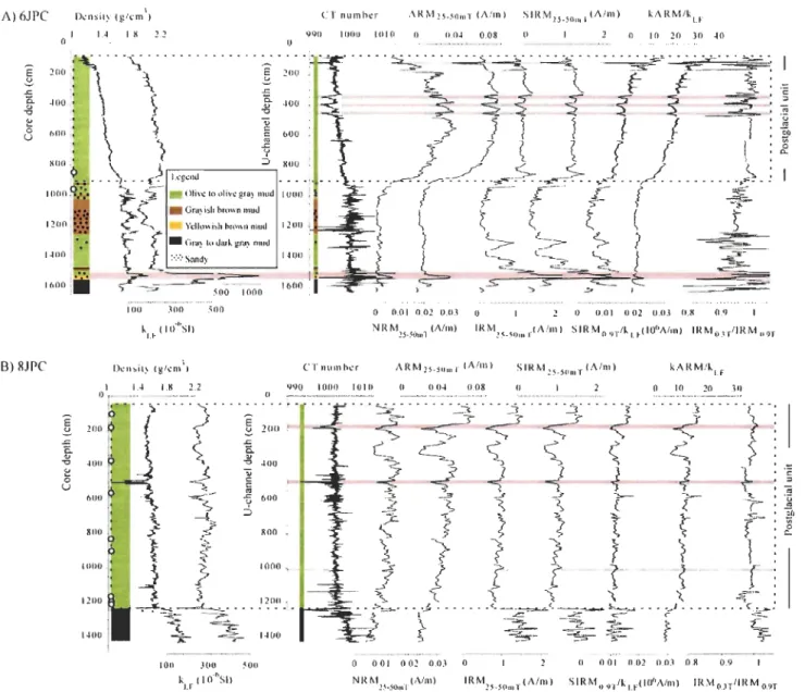
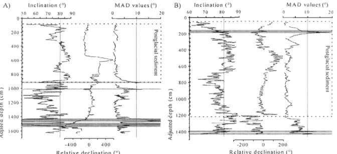
whole cores, whereas the magnetic remanence values (NRM, ARM, IRM) were measured on u-channel samples ... 15 Figure 3. Downcore physical and magnetic properties with simplified lithology of cores a) 6JPC and b) 8JPC. The upper dashed rectangle indicates the postglacial sedimentary unit of each core. Unreliable intervals are highlighted in gray (see text for details). Circles along the core depth axes represent the location ofradiocarbon dated material as listed in Table 2 ... 16 Figure 4. AF demagnetization behavior and orthogonal projection diagrams of sampI es from the postglacial (top) and the basal (bottom) units of cores a) 6JPC and b) 8JPC. Open (close) circles denote projections on the vertical (horizontal) plane ... 17 Figure 5. Downcore variation of ChRM inclination, declination and MAD values of cores a) 6JPC and b) 8JPC. The vertical line on the inclination graph indicates the expected GAD value for the latitude of the sampling site. The dashed rectangle indicates the postglacial sedimentary unit of each core. Unreliable intervals are highlighted in gray (MAD values> 100

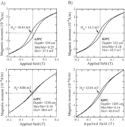
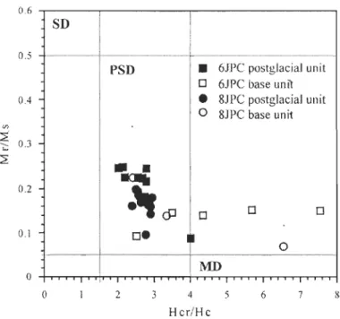
) .. . . ... . . .... . . . 18 Figure 6. Typical hysteresis curves and derived parameters for the postglacial unit (upper graph) and the basal unit (lower graph) of cores a) 6JPC and b) 8JPC ... 20 Figure 7. Day plot (Day et al., 1977) of cores 6JPC and 8JPC pilot samples. AIl samples from the postglacial units (solid symbols) faIl in the pseudo-single domain (PSD) range for magnetite ... 21 Figure 8. Magnetic grain size indicator SIRM vs

hF

for cores a) 6JPC and b) 8JPC. The

reference hnes for magnetite are from Thompson & Oldfield (1986) ... 22 Figure 9. Changes in magnetic concentration in the postglacial unit of cores a) 6JPC and b) 8JPC. The variability on each axis is indicated. A variability lower than one order of magnitude is required for paleointensity determination (Tauxe, 1993) ... 23 Figure 10. Radiocarbon-based age model of core 8JPC. Linear fit (dashed lin es) equations and estimated sedimentation rates (SR) are indicated. The excluded date is shown with an open symbol. ... 24

Figure 11. Nonnalized intensity for cores A) 6JPC and B) 8JPC. Gray intervals highlight where the three nonnalization parameters result in different relative paleointensity behavior. ... 27 Figure 12. Coherence of the relative paleointensity proxies with their nonnalizers for cores A) 6JPC and B) 8JPC. The horizontalline represents the 95% confidence level. A Blackman-Tuckey cross-spectral analysis using a Barlett window (Paillard et al., 1996) was applied. NRM₂₅_

50mT ISIRM25-50mT VS SIRM25-50mT (not shown) is similar to NRM25-50mT IIRM25_50mT VS IRM25-50mT' ... 28 Figure 13. Figure 13. Full vector paleomagnetic comparison of cores 6JPC and 8JPC with regional records on their own chronology. Core 6JPC is shown with its adjusted depth scale. A) Inclination, B) Declination and C) Relative paleointensity records from Western North

American volcanic rocks (PSVL; Hagstrum and Champion, 2002), Grandfather Lake

sediments, Alaska (GFL; Geiss and Banerjee, 2003), Beaufort Sea and Alaskan margin sediments (cores 803 and 5JPC; Barletta et al., in press), Mara Lake sediments, Western Canada (MR; Turner, 1987). AIso illustrated are the cals7k spherical harmonie outputs for the Alaskan margin (derived from Korte and Constable, 2005). The Mara Lake chronology was calibrated using the IntCalO4 calibration curve (Reimer et al., 2004). The pale line on the Alaskan margin plots (5JPC, 6JPC and 8JPC) represents the high resolution records and the dark line represents an Il points moving average function. Correlative features discussed in the text are illustrated ... 30 Figure 14. Depth vs age diagram of core 6JPC based on the identified paleomagnetic tie points (Table 3) considering an offset of A) 80 cm and B) 147 cm between the piston (6JPC) and the trigger weight (6TC) cores. Both age models fall within the error bar limits of the available radiocarbon date (Table 2) shown with a thicker symbol. The black li ne is an interpolation between points or cluster of points (Ortiz et al., this issue) and the dashed line represents a linear fit in aIl the points. The linear fit equation and derived sedimentation rate (SR) for the two possible adjusted depth-scales of core 6JPC (dashed line) are illustrated for comparison . ... 34

Introduction générale

La variabilité du champ magnétique terrestre

L'échelle des temps de polarité géomagnétique (geomagnetic polarity timescale;

GPTS) est un outil efficace de stratigraphie pour des périodes couvrant plusieurs millions d'années. Une telle magnétostratigraphie globale n'existe pas pour la variabilité à haute fréquence du champ magnétique terrestre. D'abord, quelques siècles ne suffisent pas pour

observer des inversions de polarité ou des excursions magnétiques. Ensuite, des

dissimilitudes ou des décalages temporels peuvent être observés entre des enregistrements paléomagnétiques à haute fréquence venant de régions différentes du globe. La contribution

non-dipolaire du champ magnétique terrestre et la superposition de sIgnaux

environnementaux ou climatiques pourraient être à l'origine de ces différences d'un continent à un autre ou sur quelques milliers de km seulement (e.g., Lanza et Meloni, 2006). Ainsi, la distance géographique maximum pour laquelle des variations millénaires de paléointensité relative sont généralement cohérentes est de quelques milliers de kilomètres (Lund and Schwartz, 1999). L'étude du paléomagnétisme à partir de séquences sédimentaires est le seul moyen d'obtenir un enregistrement continu dans le temps et lorsque le taux de sédimentation est suffisamment élevé (> 1 00 cm/ka), une résolution millénaire à séculaire de la variabilité du champ magnétique passé peut être atteinte (e.g., Stoner et al., 2007, St-Onge et al., 2003; Barletta et al., sous presse).

La magnétostratigraphie

holocène

L'étude des variations millénaires à séculaires du champ magnétique est un moyen de mieux comprendre la variabilité de haute fréquence du champ magnétique de la Terre, mais

peut aussi permettre de développer des traceurs paléoenvironnementaux (e.g.,Verosub and

Roberts, 1995) ou un outil stratigraphique robuste (e.g., Guyodo and Valet, 1996, 1999; Laj

et al., 2000; Stoner and St-Onge, 2007). Un avantage de la magnéto stratigraphie est que

l'enregistrement du vecteur magnétique (inclinaison, déclinaison et paléointensité) est indépendant du contexte environnemental. Que les grains magnétiques se déposent en milieu

marin ou lacustre (i.e., magnétisation rémanente post-déposition; pDRM) ou qu'ils se trouvent dans une coulée de lave ou dans une poterie d'argile cuite (i.e., magnétisation

rémanente thermale; TRM), ils enregistrent au même moment la même information

magnétique. La principale différence entre les deux types de magnétisation rémanente ci-dessus est que l'enregistrement de l'intensité du champ magnétique par TRM est ponctuel et absolu, alors que l'enregistrement par pDRM est continu et relatif. Ainsi, des données

archéomagnétiques bien datées tels des évènements volcaniques connus peuvent servir à calibrer des enregistrements paléomagnétiques continus. De manière générale, la

comparaison d'archives paléomagnétiques provenant de différents contextes (e.g., lave et sédiments) et/ou de différents environnements (e.g., sédiments marins et sédiments lacustres)

permet de valider les données obtenues pour une région donnée (e.g., Bohnel and Molina-Garza, 2002 ; Hagstrum et Champion, 2002 ; St-Onge et al., 2003 ; Herrero-Bervera et Valet, 2007 ; Barletta et al., sous presse). La reproductibilité constitue d'ailleurs un critère de qualité important pour un enregistrement sédimentaire de paléointensité relative (King et al., 1983; Tauxe, 1993).

Un autre avantage important de la magnéto stratigraphie est son utilisation comme outil chronostratigraphique dans des environnements où les techniques de datations

conventionnelles pour la période Quaternaire (e.g., datations radiométriques, comptage de

varves) sont difficiles ou inapplicables. Par exemple, les sédiments ne sont pas toujours

varvés et du matériel carbonaté n'est pas toujours trouvé pour effectuer la datation du radiocarbone (14C). De plus, l'effet réservoir en milieu marin ou la contamination par du

« vieux carbone» en milieu lacustre ne sont pas toujours bien documentés et peuvent

introduire d'importantes incertitudes (e.g., Snyder et al., 1994; Walker, 2005 ; Mangerud et al., 2006). Dans de tels environnements, il est donc optimal de combiner les méthodes de datations conventionnelles avec des indicateurs chronologiques (e.g., tephra, pollen,

magnéto stratigraphie ).

Finalement, la magnéto stratigraphie peut atteindre de très hautes résolutions

trouve les archives paléomagnétiques aux plus hautes résolutions temporelles dans certains

lacs et sur certaines marges continentales où s'accumulent des sédiments en grande quantité

depuis la dernière glaciation et déglaciation. Un nombre croissant d'études paléomagnétiques

sur les sédiments holocènes de ces endroits clés ont été publiées depuis quelques décennies et des courbes de références régionales ont aussi été construites (e.g., Turner and Thompson,

1981 ; Creer and Tucholka, 1982; Lund and BaneIjee, 1985; Verosub et al., 1986; Lund,

1996 ; Gogorza et al., 2000 ; Snowball and Sandgren, 2002 ; Snowball et al., 2007 ; Stoner et al., 2007). Bien que des sédiments holocènes se soient accumulés avec des vitesses de

sédimentation élevées à certains endroits des mers épi continentales Arctiques (Hill et al.,

1991 ; Darby, 2006), très peu d'études publiées à ce jour proviennent de sédiments des hautes latitudes nord (>600_{N) et la majorité d'entres elles sont basées sur des sédiments}

lacustres.

Le paléomagnétisme en Arctique

La datation de séquences sédimentaires est souvent problématique en Arctique

puisque la dissolution du matériel carbonaté raréfie la conservation de coquilles ou de tests

dans le sédiment (Jutterstrom et Anderson, 2005). Lorsqu'il y a datation de matériel carbonaté, il est nécessaire de corriger l'âge radiocarbone apparent pour le temps de résidence du CO2 dans l'eau. Cet effet réservoir est mal connu dans les différentes régions de l'Arctique

et peut varier dans le temps (e.g., Bjork et al., 2003; Ericksson et al., 2004; Poliak et al.,

2007). Dans ce contexte, l'utilisation d'indicateurs chronologiques est un bon complément

aux datations radiocarbones. En ce sens, Barletta et al. (sous presse) ont récemment démontré

le potentiel d'utiliser la variabilité millénaire à séculaire du champ magnétique terrestre en

Arctique de l'Ouest pour développer des marqueurs chronostratigraphiques régionaux. Le paléomagnétisme aux hautes latitudes est d'autant plus intéressant que les variations

d'inclinaison et de déclinaison sont de plus grande amplitude à proximité du pôle Nord

géomagnétique, ce qUI pourrait faciliter l'identification de tels marqueurs

Le paléomagnétisme en Arctique est prometteur puisque les sédiments postglaciaires qui s'y trouvent contiennent généralement des grains fins de magnétite et de titano-magnétite

(Darby, 2003; Darby and Bischof, 2004; Bischof and Darby, 1997, 1999), d'excellents minéraux magnétiques pour l'acquisition d'une pDRM et pour les reconstitutions d'orientation (inclinaison et déclinaison) et de paléointensité relative (Tauxe, 1993 ; Stoner et St-Onge, 2007).

Les objectifs de ce projet de maîtrise sont de

1) reconstruire et décrire la variabilité du champ magnétique terrestre en Arctique de l'Ouest

selon deux séquences sédimentaires de la marge continentale de la mer de Chukchi;

2) établir par magnéto stratigraphie la chronologie de la séquence sédimentaire HL Y050

Chapitre 1

Paleomagnetic constraints on the Holocene stratigraphy

of the Arctic

Alaskan margin

Agathe Lisé-Pronovosta,b*, Guillaume St-Ongea, b, Stefanie Brachfeldc, Francesco Barlettaa, b,

Dennis Darbl

a Institut des sciences de la mer de Rimouski (ISMER), 310 allée des Ursulines, G5L 3A l,

Rimouski, QC, Canada

b GEOTOP research center

C Montclair State University, NJ, USA

ct Dept. of Ocean, Earth, & Atmospheric Sciences, Old Dominion University, VA, USA

*Corresponding author: agathe.lisepronovost@ugar.gc.ca

Keywords: Paleomagnetism, Arctic, Holocene, paleomagnetic secular variation, relative

paleointensity, marine sediment

Abstract

Two long Holocene piston cores (HL Y050 1-06JPC and -08JPC) were raised from high sediment accumulation areas at the Arctic Alaskan margin in order to reconstruct the millennial- to centennial-scale behavior of Earth's magnetic field and to better constrain the regional chronostratigraphy of the Western Arctic. Paleomagnetic and physical analyses indicate that both sedimentary sequences have recorded a reliable record of paleomagnetic secular variation (inclination

and declination) and relative paleointensity during the Holocene. The accelerator mass spectroscopy

(AMS) radiocarbon-based postglacial chronology of core HLY0501-08JPC indicates sedimentation rates as high as 348 cm/ka on the continental shelf near Barrow Canyon from approximately 8000 to 5000 cal BP, followed by a major decrease in sediment deposition. Full vector paleomagnetic correlation (inclination, declination and relative paleointensity) was used to constrain the chronology

of core HL Y050 1-06JPC, using core HL Y050 1-08JPC and other previously published and independently dated sedimentary and vo1canic records from Western North America.

1. Introduction

The study of millennial to centennial variation of the Earth's magnetic field recorded by sedimentary sequences is a means of better understanding the geomagnetic field high frequency behavior, and can be a very useful stratigraphic tool (e.g., Guyodo and Valet, 1996,

1999; Laj et al., 2000; Stoner and St-Onge, 2007). In the last few decades, an increasing number of Holocene paleomagnetic studies based on marine and lacustrine sediment sequences have been published. In an effort to further develop magnetostratigraphy as a regional dating tool, Holocene paleomagnetic reference curves have been constructed for the United Kingdom (inclination and declination; Turner and Thompson, 1981), Sweden (inclination, declination and relative paleointensity; Snowball and Sandgren, 2002), Finland (inclination, declination and relative paleointensity; Snowball et al., 2007), North America (inclination and declination; Lund and BaneIjee, 1985; Verosub et al., 1986; Lund, 1996),

East-central North America (inclination and declination; Creer and Tucholka, 1982) and South Argentina (inclination and declination; Gogorza et al., 2000). In parallel, Korte and

Constable (2005) developed a global geomagnetic field model (CALS7K.2) based on

spherical harmonic analysis. This model was calibrated with archeomagnetic (from volcanic

rocks and fired artifacts) and paleomagnetic (from sediment sequences) data for the last 7 kyr

and it has succeeded in reproducing sorne of the millennial- to centennial-scale dipole

moment variability observed in the sediment sequences (Korte and Constable, 2006).

The observation of synchronous changes of the geomagnetic field, either inclination,

declination and/or intensity at sites from the same area can lead to the identification of

regional chronostratigraphic markers. For example, Barletta et al. (in press) recently observed

several directional and paleointensity features that have the potential to be used as

chronostratigraphic markers for Holocene sediments in the Western Arctic. Such markers are

especially attractive in the Arctic, where dating is often complicated (see below). Due to their

proximity to the North geomagnetic pole, the high latitude sites have the potential to record

higher amplitude directional changes than in the lower latitudes. Unfortunately, only a

handful of paleomagnetic studies covering the Holocene period have been published from

northern high latitude sites (> 600N) and only a subset of these present the full paleomagnetic

vector (Andrews and Jennings, 1990; Frank et al., 2002; Snowball and Sandgren, 2002; Geiss

and Banerjee, 2003; Nowacyzk et al., 2001; Snowball and Sandgren, 2004; Snowball et al.,

2007; Stoner et al., 2007; Barletta et al., in press). Because high sedimentation rate sites are

found on the continental shelves and si opes of Arctic marginal seas (Darby et al., 2006), these

sites are key are as to address the millennial- to centennial-scale geomagnetic field variability

for the Holocene.

The prerequisite for a paleoclimatic study based on a sedimentary sequence is the

establishment of a reliable age model in order to transform the depth scale into an age scale.

Since the radio carbon reservoir effect is often poorly constrained in the Arctic and since the

datable material is often very rare, the chronostratigraphy of Arctic marine sediment

sequences has always been a challenge. It is therefore optimal to combine dating methods.

High-resolution magnetostratigraphy is a valuable tool to date sediment sequences in the

absence of datable material (e.g., Mackereth, 1971; Saarinen, 1999; St-Onge et al., 2004) or

to independently support and improve a chronostratigraphy based on radiocarbon dating (e.g.,

Creer and Tucholka, 1982; Andrews et al., 1986; Kotilainen et al., 2000; Stoner et al., 2007).

In this paper, we present the full vector paleomagnetic records (inclination, declination and

relative paleointensity) of two long Holocene piston cores in order to cons train the

2. Regional setting

The two studied jumbo piston cores were recovered from the Arctic Alaskan margin in the eastern Chukchi Sea (Fig. 1). A distinct submarine feature in the area is the Barrow Canyon, a major pathway for dense Pacific water inflow from the Bering Strait (Pickart et al., 2005) and for sediment loaded waters moving from the continental shelf (Weingartner et al., 1998) toward the continental slope and the Canada Basin. In the present oceanographic conditions, upwelling events of intermediate-depth Atlantic waters from the Canada Basin into the Barrow Canyon have been observed episodically (Pickart et al., 2005).

70'N l20"W IOO'W Bathymetry Bilo-som _ S1-100m . 101-200m _ 201·500m _ 501·2500m _ >2500m ~O"w

Figure 1. Location of cores 8JPC and 6JPC in the Western Arctic Ocean as well as other high resolution Western North American records cited in the text: 5JPe and 803 (Barletta et al., in press), PSVL (paleosecular variation from lava flows; Hagstrum and Champion, 2002), ML

(Mara Lake; Turner and Thompson, 1981) and GFL (Grandfather Lake; Geiss and Benerjee,

Since the manne transgression (from about 12000 cal BP on the Chukchi shelf;

Keigwin et al., 2006) associated with the last deglaciation, the major sediment sources on the

Arctic Alaskan margin come from river discharge, coastal erosion and redistribution of sediment by ice drift. Northern North American rivers bringing sediment at the Arctic Alaskan margin are found from the Beaufort Sea to the Bering Sea. The Colville River in

Alaska (USA) and the Mackenzie River in the Northwest Territories (Canada) are major

rivers forming deltas in the western Arctic Ocean. However, smaller rivers located in northwest Alaska (Utukok, Kokolik and Kukpowruk Rivers) are reaching Barrow Canyon through a network of submarine paleochannels and would have been an important sediment source to the northeast Chukchi Sea during the last deglaciation (Hill and Driscoll, 2008).

Due to the present hydrodynamic conditions, most of the Chukchi shelf is the area of net

seafloor erosion or non-deposition, whereas fine-grained sediments are deposited in the valleys such as the Barrow Canyon and deeper on the slope (Phillips et al., 1988). Grains are also transported and released in the Chukchi Sea by sea ice (Darby and Bischof, 2004; Darby, 2003).

The last major lithostratigraphic marker on the Western Arctic margins is the

lithological change associated with the transition from deglacial to marine Holocene

environments (e.g, Darby et al., 1997; Polyak et al., 2007). Previous geophysical seafloor

surveys and core descriptions from the Chukchi Sea have shown that brownish to olive-gray,

strongly bioturbated mud (postglacial sediments) overlay stiffer grayish, sometimes

laminated mud containing ice rafted debris (glacial/deglacial sediments) in the Chukchi Sea

(Philips et al., 1998; Keigwin et al., 2006; Polyak et al., 2007). Similarly, Barletta et al. (in press) described a piston core from the Chukchi Sea with about 12 meters ofpostglacial olive gray mud overlying glacialldeglacial sediments.

3. Materials and Methods

3.1. Coring sites

Two long jumbo piston cores (HL Y050 1-06JPC and HL Y050 1-08JPC, hereinafter referred as to cores 6JPC and 8JPC, respectively, Table 1) from the Arctic Alaskan margin

were collected on board the US CGC Healy as part of the 2005 Healy-Oden Trans-Arctic

Expedition (HOTRAX). The Alaskan margin coring sites were selected using the

hull-mounted 3.5 kHz subbottom profiler and the 12 kHz multibeam bathymetric sonar for the areas of significant thickness (> 1 0 m) of apparent Holocene sediments, as previously observed in the area (Phillips et al., 1988; Keigwin et al., 2006), and for the absence of

erosional features or sediment deforrnation by mass movements. Core 8JPC was raised from

the continental shelf (90 m) near the Barrow Canyon, while core 6JPC was collected ~100

km northwards in the lower mid-slope (673 m; Table 1; Figure 1).

Table 1. Core location.

Core Latitude (ON) Longitude (0W) Localisation Water depth (m) Length (m)

HLY0501-06JPC 72.69 157.03 Lower mid-slope 673 15.54

-06TC HLY0501-08JPC -08TC 71.63 3.2. Physical analysis 156.86 Continental shelf 90 1.03 13.96 3.06

On board, the piston cores were analyzed with a GEOTEKTM Multi Sensor Core

Logger for the deterrnination of wet bulk density (by gamma-ray attenuation) and low-field

volumetric magnetic susceptibility (kLF) at 1 cm intervals, then split and described. kLF is mainly proportional to the ferrimagnetic mineraI concentration. However, kLF increases with paramagnetic material when the concentration of ferrimagnetic material is low and with the addition of superparamagnetic

«

0.03 /lm) and large (> 10 /lm) magnetite grains (e.g., Thompson and Oldfield, 1986; Stoner and St-Onge, 2007). In the laboratory, the cores were

photographed with a high resolution digital camera and sampled with u-channels (u-shaped

plastic liners of 2 x 2 cm cross-section and up to 1.5 m length). The u-channels were then

de la Recherche Scientifique, Centre Eau, Terre, Environnement (INRS-ETE) in Quebec city,

Canada, in order to visualize the sedimentary structures, possible core deforrnation and

extract the computed tomography (CT) numbers. The CT number primarily reflects changes

in bulk density with al-mm downcore resolution (St-Onge et al., 2007).

3.3. Paleomagnetic analysis

Paleomagnetic data were acquired at 1 cm intervals on u-channel samples using a 2G

Enterprises™ cryogenie magnetometer and pulse magnetizer module (for Isotherrnal Remanent Magnatization, IRM) at the new Paleo and Environmental Magnetism Laboratory

at the Institut des sciences de la mer de Rimouski (ISMER), Canada. The response function of

the magnetometer pick-up co ils integrates measurements over - 4.5 cm (Weeks et al, 1993).

To eliminate the edge effect associated with this response function, the first and last 5-cm

data of each u-channel were excluded.

The natural remanent magnetization (NRM) was measured first usmg stepwise

altemating field (AF) demagnetization at peak fields from

°

to 70 mT at 5 mT increments.

Inclination and declination of the characteristic remanent magnetization (ChRM) were

ca1culated by a least-square line-fitting procedure (Kirschvink, 1980) using the Mazaud

(2005) software with AF demagnetization steps from 20 to 70 mT (11 steps). An anhysteretic

remanent magnetization (ARM) was then induced at peak AF of 100 mT with a 0.05 mT

direct current (DC) biasing field and subsequently demagnetized and measured at 0, 10, 15,

20, 25, 30, 35, 40, 45, 50, 55, 60, 65, 70 mT. An isotherrnal remanent magnetization (IRM)

was imparted with a DC field of 0.3 T and subsequently demagnetized and measured at 0, 10,

15, 20, 25, 30, 35, 40, 45, 50, 55, 60, 70 mT. Similarly, a second IRM (corresponding to a

Saturated Isotherrnal Remanent Magnetization, SIRM) was imparted with a higher DC field

of 0.9 T and then demagnetized and measured at 0, 10, 20, 25, 30, 35, 40, 45, 50, 60, 70 mT.

The arithmetic mean of each magne tic remanence (NRM, ARM, IRM and SIRM) for the

demagnetization steps 25 to 50 mT (6 steps) is presented in figure 3.

Hysteresis properties were measured on pilot samples from core section breaks using

a Princeton Measurements COrp.TM vibrating sample magnetometer (VSM-3900-04C) at 10

mT increments with a maximum field of 1 T at Montclair State University in New Jersey,

USA, in order to help constrain the magnetic mineralogy and granulometry. The following

coercivity of remanence (Hcr) , the saturation magnetization (Ms) and the saturation remanence (Mr).

AIl laboratory-induced magnetizations are dependant on the concentration of magnetic material present in the sample, but each type of magnetization activa tes a specific

group of magne tic grains. Alone or normalized by another magne tic parameter, the different

magnetizations are thus useful to characterize variations in magnetic mineralogy and

granulometry (e.g., King et al., 1982; Thompson and Oldfield, 1986; Brachfeld and Banerjee,

2000; Maher et al., 1999; Peters & Dekkers, 2003; Stoner and St-Onge, 2007). SIRM

normalized by the magnetic susceptibility (kLF) is an indicator of the magnetic grain size,

with smaIler values denoting coarser magnetic grains (Thompson & Oldfield, 1986). kARM is

ca1culated by dividing the ARM by the strength of the DC field applied and is also used as a

magnetic grain size indicator when divided by kLF, where kARM/kLF is inversely proportional

to the magnetic grain size if the magnetic mineralogy is mainly magnetite (King et al., 1982).

FinaIly, 1RMomT 0.3T normalized by SIRMomT 0.9T (pseudo S-ratio) is an indicator of the

magnetic mineralogy, with values close to 1 denoting low coercivity mineraIs such as

magnetite (e.g., St-Onge et al., 2003). The median destructive field (MDF) is the required

peak field to reduce the initial magnetic remanence by half. The MDF is a magnetic mineralogy indicator depending on the coercivity of magne tic mineraIs and on the magnetic gram Slze.

3.4. Radiocarbon analysis

Accelerator Mass Spectroscopy (AMS) radiocarbon measurements were performed on

9 moIlusk sheIls (core 8JPC, Table 2) and on benthic foraminifers (core 6JPC, Table 2) at the

Lawrence Livermore National Laboratory's Center for Accelerator Mass Spectroscopy (LLNL-CAMS) and at the NSF-Arizona Accelerator Mass Spectroscopy Laboratory. The

dates are reported using Libby's half-life and corrected for natural and sputtering

fractionation (ÔI3_{C = -25%0 vs. VPDB). To convert the 14C ages to calendar years, the dates}

were calibrated using the CALIB5.0.2 on-line calibration software (Stuiver et al., 2005),

assuming a ~R of O. The calibrated ages are reported at the 2a confidence level. Based on

paleomagnetic data, a ~R of 0 was recently shown to be appropriate for a nearby Arctic

Alaskan margin core (Barletta et al., in press). Nonetheless, uncertainties remain about the

where there is a possible Pacific component (e.g., shallower waters on the Alaskan margin;

core 8JPC) should be considered as maximal ages.

Table 2. Radiocarbon dates from cores 6JPC and 8JPC

Core Depth Adjusted depth Dated material Lab number AMS 14C age Calibrated age"

(cm) (cm) (yr BP) (yr cal BP)

HLY0501-06JPC 770-772 850-852 Benthic forams CAMS135962 7690 ± 180 7790 (8160) 8520

878-880 958-960 Benthic forams AA74466 12375 ± 60 13710 (13850) 13980

HLY0501- 51 102 Bivalve Macoma AA66974 3216 ± 37 2900 (3030) 3160

08JPC 130 181 Bivalve Astarte CAMSI37887 4590 ± 30 4700 (4790) 4880

327 378 Bivalve Nuculana CAMSI37888 5210 ± 30 5480 (5560) 5640

510 561 Bivalve Macoma AA66975 5309 ± 79 5530 (5710) 5880

789 840 Bivalve Macoma? CAMSI37889 5995 ± 35 6300 (6400) 6500

851 902 Bivalve CAMSI37890 6110 ± 40 6430 (6540) 6650

1116 1167 Bivalve CAMSI37378 7285 ± 35 7660(7750)7840

1150 1201 Gastropode Natica? AA66976 7760 ± 51 8110 (8230) 8350*

1153 1204 Bivalve CAMSI37891 7415±35 7790 (7880) 7960

a The conventional ages were calibrated with the CALIB5.0.2 (Stuiver et al., 2005) online calibration software using the Hughen et al. (2004) dataset and assuming a.0.R value of 0 (see text for details). The tirst and last ages represent the 2a cal age range rounded to the nearest tens, whereas the ages in parentheses are the average age rounded to the nearest tens. * = excluded age.

4. Results

4.1. Core stratigraphy

Correlation of the physical and magnetic parameters measured on the piston cores (JPC) and their companion trigger weight cores (TC) suggests that 51 cm and 80 cm of sediments were lost due to coring at the top of cores 8JPC and 6JPC, respectively (Fig. 2).

The missing piston core sediments were taken into account and aIl depths hereinafter are expressed as adjusted depth if not otherwise specified. Because of significant sediment disturbances in the u-channel sampled from the trigger weight core 6TC, only measurements from the who le core (i.e. MSCL measurements) were used for correlation purposes of cores 6JPC and 6TC. A higher sediment lost (147 cm) at the top of core 6JPC is also possible and suggested by the diffuse spectral reflectance data (Ortiz et al., this issue). Even thought the depth scale is here presented using an adjustment of 80 cm, the possible higher sediment loss is also taken into account for the construction of core 6JPC age model (see section 5.5).

A significant change in aIl the physical and magne tic parameters occurs at 935 cm in core 6JPC and 1230 cm in core 8JPC (Fig.3). The top sedimentary unit of both cores is characterized by olive gray to dark olive gray fine mud to sandy mud. These sediments are typical of Arctic shelf postglacial sediments (e.g., Syvitski, 1991; Darby et al., 2006; Keigwin et al., 2006; Barletta et al., in press). In addition, numerous black iron sulfides are found within this unit. The basal sedimentary unit of core 8JPC is composed of gray to dark gray,

stiff mud with sand and coarser grains, suggesting deposition in a glacial/de glacial regime and/or in nearshore environments during the sea-Ievel rise. In core 6JPC, the bottom of the top unit occurs at 935 cm and the first centimeter-scale drop stone is found above this transition, at 910 cm. Other dropstones are found at 1132 cm and 1290 cm, whereas ice rafted debris (IRD) are common from 1515 cm to the end of the core. Between 935 and 1515 cm,

the sediment is composed of brown and olive gray mud laminations where sand and bioturbated contacts are found, which is typical of glaciomarine sediments (Syvitski, 1991). This interpretation is supported by an age of 13 850 cal BP at 858-860 cm (Table 2). From 1515 to 1535 cm, a yeIlowish brown sandy mud horizon with IRD is observed and has a relatively higher concentration of high coercivity magnetic mineraIs as shown by a sharp decrease in the pseudo-S ratio (gray interval at the base of Fig. 3a). Below this horizon, the

A) 6TC-6JPC 6TC dcnsity Cg/cm) 90 110 130 150 1.1 1.2 t.3 -8 () -80+--'---'----'----'---+ · .... ····.t . . ,;!. R=O.94 E; 0 u ~ 80 c-_...., E ~ () c-100 - ; ()

-::

c.. fi Cl-c.. ₈₀

'"

"0

"

c.. _&0 160 ~ IV

:;,-"

"0 " ~ U 0.. -c 1 60-~ U (") _0.. '3 ..., 160-240 ~ '0 240- .120 240-100 140 1 &0 220 1.3 14 1.5 6JPC k_LF (l 0·6S1) 6JPC density (g/cm') JPC B) 8TC-8JPC _TC 8TC k _I..F . (10-6 S1) 8TC NRM_30mT (A/m) 220 260 300 340 _0.08 lI.12 0.16 0.2 ·50 0 _{·50 0} R=O.89 _R;:0.71 .... ',~ .... :.:,' ',:,::.',,: ',' .. 0

'--<

., ... >

'"

00 S

-==

<2

/

:.:~·::

>

·'

00

2

-1 _<>

ri

.:1 10ù () ~ -5 .. 0- -:: _{50 100} 0. c.. _" 0.

-=c~5

'

=

" '" .' "0 " "0 "0 ₁₀ ::T "0 :;,-U ,... U ~ "'- " 0.. 10 _" .., 3 .... :3 00 ₂₀₀ 00 15 200 20 J40 180 220 260 _{0.06 0.1 0.14} 8.1 PC k_LF (1 0-6 S 1) 8JPC NRM _{30m T (Alm)} 8TC ARM_30mT(A/m) STC lRM_30mT (A/m) 0.1 0.3 0.5 0.7 6 10 14 ·50 ·50 0 R=O.91

..

' R=O.91 .':: . 1'0' 0

.. >

'"'" 0 E ce E 00

.::--=s

-1 ~

)

-1 () ()

-=

Cl. ..r:: Cl. Cl. ₅₀ : _{100 ~} c.. _{50 100} " <>

"

v

"

=- v _{: ~} U ,... U ,... Il.- !::: 0.. (") ... ₁₀ ::: .., _{10 3} 00 00 15 200 15 200 0.2 04 0.6 0.8 10 15 8JPC NRM_{30rnT (}A/Ill) 8JPC IR M_30mT (A/m)

Figure 2. Correlation of the physical and magnetic parameters between the jumbo piston core

(JPC) and its trigger gravit y core (TC) plotted with a 5 points moving average function. The magnetic susceptibility (kLF) and bulk density measurements were acquired on board on

whole cores, whereas the magnetic remanence values (NRM, ARM, IRM) were measured on

1-' en A) 6.JPC Dcnsity tg/cm}

,

CT numh~r /\RMlS,Sn",,. (AllO 1 SIRM_15,5n",.,.,A/m) kA RM/k1.F E ~ ..c: 1 o 200 1.4 1 X 1.1 9QC) IU(H' 11110 Il.04 0.08 10 20 30 40

\

'

,

'~\"

, , ,

,

,

, , ,

,

, ,

i

'2'(1;, " .. , , :~

i

'~'Z~X(

.. , \'

, , ,

,

t~~·, {~'';-'

,

'r

.~ a 4110 .g

' f

l ! '0

g.

400 . , ,. ~ _~ ~

.:2

~ __

._

<

~

_

<

<:

_

_

~ 5 :5 ~ ~~~~_:. ._ ~ ~ a U bOUT \ ) ] 600 '''}

!

1 1

?

1

1 :

~

.,,"

L

I

\

d,

qe

"

~

.,,

"

l

-l-/~

-

tJ

Jj

J

j •

,

oon~

~

;;;.~

. O'l\o,ollll\ogra) mlld 'UIIII !

,

f;'

f

r r ;:

f

f

1

nun

14no

jr. •••

1600

1

.

..". .... • Gru~ "h bru". II1l1d t ! ~ t ~ (

1-ç ~ YdhmishtHO\\lInlml IlUtl "'-1 :::;;;;;;;~ii;.-~ ~ \ \ ~ )

f'"

r.

GI~! ,,, dark grny mud ~)

>

>

'>

1

--=~

fJ

l

:';':'Sond)' 141H1 ~.- ~ L~ C~ ~

l

-Z

.... - ~ ~ -=--, ~-

-_

r

~~ 1600 l' . ..s. .s: =Z:::_' ~ --_.~ ~ --:::=.r ~ 00 1000 ) ) ':) ":':lo ::. J , .... , - -... _,_ ... -_. 101) 300 ,00 _{0.01 0.02 0.113 11.01 0.01 0.03 Il.X 0'1} k _1.. (IO'"s1l NRM_15.;O",' (A/m) IRII\;,;O",,.,Alml SIRMo,,.,./l,,,(Hl';A1tnl IIIMon/IRMII9T

B) 8JPC Dcn~il~ Ig/cm', CT num h~r ARM15.~Uml' tA/m) SIRM 25,"'",T IA/m) kA RM/kl.F

E ~ ..c: _a '" "C ~ a U 1 o 200 400 hOU 800 11H10 1200 1400 1 A I.X 1.2 Q90 101111 1010 11.0~ IUI8 _.. _._._.10 _ ...

-

_

_..

_

20

-

-

_

3_...1t _• '~" '"

«

'.' i " " " ' "

'

t

"""

":::,.:

"""

'..:..-:i" " '_3" ' " '..:J" ' " '' i '' ' ' ' ' ' )' ''' . ' ( ' " 1

~

100 !

~

-

<

<

-

~y

-

<

-<

~

:

~ fr è~

<..

C;

c;:

? ? , '" '0 400 "':>:.:> ~ > ' : ; . . . , • _

-

~

l

,

-

'

-l

-=!

~ ~

-{

-

-

1

+

:~

-<.Ç

~ 600 ~

-t

-~ ~

'{

r-t-

:

]

1

~

KOO •

<-

J

?

?

t

~

r

:

~n

~

) '[ ? ?

}

?

1

} 1000, - ;-

I

t l

-

t

' -

-

i

-

-

f

~ 1 21'" . _ '\. (" '\ '\ \ \ ff."'- , _ .. '---:_ • • • • • •• • '. .. • • • ">~ • • • • ..t •••..•. (. ____ ~('.--_h~ ... . ,..1 ••••••• • "..!'! . .-.. --;;=-_~ ~_.'!. 1 _.~:..~~~ ~ c- ~ _~ -===- -..,? .- 1400. ~ !. ?l.. ~-__ ~:;,..::-_ :s: f ~ "-J ~-~----100 ),,0 300 0.01 0.02 0.03 0.01 0.01 n.nJ 0.8 0.9 k (1 O··SiI

Lf N((~l 1~·50IllT (Mill) IRM H~50mT (A/m) SIR MO.9T/k Lf( Hf'Mm) IR M o.n /ill M O.~T

Figure 3. Downcore physical and magnetic properties with simplified lithology of cores a) 6JPC and b) 8JPC, The upper

dashed rectangle indicates the postglacial sedimentary unit of each core, Unreliable intervals are highlighted in gray (see text for details)' CircIes alon!! the core deoth axes reoresent the location of radiocarbon dated material as listed in Table 2.

sediment becomes dark gray stiff sandy mud with the presence of IRD. The lowermost 50 cm

contain patches with iron sulfides similar to postglacial sediments. Overall, the basal unit of

core 6JPC contains multiple lithological changes and IRD, suggesting deposition in variable

glaciaVdeglacial environments.

The following intervals were excluded from the dataset of core 6JPC postglacial unit

due to sediment disturbance or incomplete filling of the u-channel as revealed by CA T -scan

images and CT number: 121 to 127 cm, 332 to 355 cm, 385 to 400 cm and 446 to 456 cm.

Similarly, the following intervals of core 8JPC postglacial unit were excluded: 170-194 cm,

485-507 cm and 1009-1018 cm. These unreliable intervals represent only 6.7% of the

postglacial units. A) South West fUp 0.009 North .---

...

.(J,(l1 o.OOY -O.Oi Eust !l)own South '(1.01.1 ·0.013 Enst (Down 6.JPC 545 cm NRM 0 mT = 0.071 Afm NRM 25-30m" = 0.027 Afm .;:;- 0.08, - - - ,

~

" 0.06 o :~ _., 0.04 §b ~ 0.02 6JPC 50 100 Applicd field (mT) 1610cm NRM Om1"= 0.013 A/m NRM 25-;0 mT = 0.001 A/m ~ 0.012 g .~ O.UOS :~ ~ 0.004 ::; 10 40 60 Sil Applied field (IllT) B) _West/Up 0.008 S~Ol_ltl_, _ _ _ _ --..~North -0.061 South -0.046 (1.1)08 -0.061 East !Down West fUp O.Ol ·0.046 East !Dowll SJ.PC 455 cm NRM () ml' ~ 0.061 AJm NRM 25.~() ml' "" {l.OIS Alm Ê $11.(16 c o

:

§

0.04 !l ~o 0.02 ~ 8JPC 1360 cm 50 100 Applied iield (mT) NRM 0 mT = 0.050 A/m NRM 25.50 mT = 0.006 A/Ill .? 0.04 .~ "0 510.02 ~ 50 100 Applied f"icld (OlT)

Figure 4. AF demagnetization behavior and orthogonal projection diagrams of samples

from the postglacial (top) and the basal (bottom) units of cores a) 6JPC and b) 8JPC. Open

4.2. Natural remanent magnetization

A strong and stable characteristic remanent magnetization (ChRM) can be isolated in both cores between the AF demagnetization steps of 20-70 mT (Fig. 4). A weak viscous component is removed after a 15 mT or less demagnetization field. The mean postglacial

NRMomT (NRM25-50mT) for core 6JPC is 0.058 ± 0.035 (0.023 ± 0.014 A/m) and the mean postglacial NRMomT (NRM25-50mT) for core 8JPC is 0.064 ± 0.042 (0.012 ± 0.006 A/m).

4.3. Paleomagnetic directional data

The ChRM inclinations in the postglacial units of bath cores vary around the

ca1culated geocentric axial dipole (GAD) inclinations for the latitude of the coring sites (Fig.

5). The mean inclination value of the postglacial unit of core 6JPC (8JPC) is 81.4° ± 21.2°

(79.3° ± 14.4°) and the GAD inclination value is 81.1° (80.6°). The ChRM declinations were

corrected for rotation at section breaks and corrected for similar circular values (e.g., 0 and 360°) to obtain a continuous record. The declination data are relative and centered at zero

since the coring was not azimuthally oriented.

A) Inclination e) MAD values (0) B) MAD vnlucsCO)

E -=-:= _Q. " -0 -0 ~ '0' « 50 60 iO 80 90 10 20 o 10 o +-'--'-... -'-""'r-'--' 200 400 600 800 1000 1200 1400 -0 B 1600 ._'O2._. 1400 « , , , -400 0 400 ·200 o 2(J()

Relative declination (") Relative declination (C)

Figure 5. Downcore variation of ChRM inclination, declination and MAD values of cores

a) 6JPC and b) 8JPC. The vertical line on the inclination graph indicates the expected GAD value for the latitude of the sampling site. The da shed rectangle indicates the postglacial sedimentary unit of each core. Unreliable intervals are highlighted III gray

(MAD values> 10°).

The maximum angular deviation (MAD) values can be used to assess the quality of

the directional data (Kirschvink, 1980). Intervals with MAD values higher than 10° are

highlighted in Fig. 5. Only one of these intervals is found in the postglacial units, where MAD values are generally lower than 5° as recently proposed by Stoner and St-Onge (2007) for high quality Quatemary directional data. High MAD values generally reflect po orly

defined ChRM due to incomplete filling of the u-channel (e.g., from 121 to 127 cm in the

postglacial unit of core 6JPC, Fig.5) or a magnetic mineraI assemblage not suitable for

recording the geomagnetic field, for example IRD-rich layers (e.g. highlighted intervals in both cores basal unit, Fig.5).

4.4. Magnetic minera/ogy

Pseudo S-ratio values are close to 1 (Figure 3) with a postglacial mean of 0.99 and 0.98 for cores 6JPC and 8JPC, respectively. This indicates that saturation of the magnetic

assemblage is achieved in a 0.3 T field, which is typical of low coercivity mineraIs such as

magnetite. The shape of the hysteresis curves from both postglacial units (Fig. 6) is also characteristic of low coercivity ferrimagnetic mineraI like magnetite (Tauxe et al., 1996),

with saturation fields below 0.2 T. Furthermore, Mrs/Ms values ranging between 0.1 and 0.3 (Figure 7) are typical of magnetite/titanamagnetite grains (Day et al., 1977; Tauxe, 1993).

The pseudo s-ratio, the hysteresis curve and the Day plot suggest that the postglacial mineralogy is most likely dominated by magnetite. Thermomagnetic curves measured on

nearby 5JPC confirmed the presence of magnetite with Curie temperatures of 577-580 oC,

and a second phase with Curie temperatures of 360-380 oC (Brachfeld et al., this issue). This lower Curie temperature was observed only in the heating curves, and was nat reversible in

experiments mn from 25-350 oC only (Brachfeld et al., this issue). We speculate that this

indicates the presence of greigite. However, the IRMomTO.9T/kLF postglacial averages of 15.8 kA/m and 12 kA/m for core 6JPC and 8JPC, respectively, verify that ev en though iron

sulfides are present in the postglacial units, neither greigite nor pyrrhotite dominates the magnetic mineraI assemblages (Maher et al., 1999). The average MDF for the postglacial

sediments is 27.5 mT for core 6JPC and 12 mT for core 8JPC. These values are again consistent with magnetite and the presence of coarser grains in core 8JPC accounts for the lower MDFs (see section 4.5).

A) E ~ 0

a

E ... 1 v .~ Sn -2 cd :::E

....

§ 0 E o E v

tS

-1

êh

<'d Depth= 250 cm Mrs/Ms= 0.25 HCF371mT -0.1 0 0.1 0.2 Applied field (T) 6JPC Depth= 1550cm Mrs/Ms= 0.14 l'lOF 38.6 ml' ~-2~~~~--~~~~~ -0.2 -0.1 0 0.1 0.2 Applied field (T) B)

E

.

~

1 o

-

_E QJ 0 E o 2 u

ii

-1 c: ~ Depth= 352 cm MfS/Ms= 0.18 HOt= 42.5 nft" -0.1 0 0.1 0.2 Applied field (T) S.IPC Depth= 1205 cm Mrs/M.s= (J.14 Her= 40.0 OlT :::E -2~~~~ __ L-~~~~ -0.2 -0.1 0 0.1 0.2 Applied field (T)

Figure 6. Typical hysteresis curves and derived parameters for the postglacial unit (upper

graph) and the basal unit (lower graph) of cores a) 6JPC and b) 8JPC.

Higher amplitude and frequency variations of the pseudo S-ratio in the basal units of

both cores (Figure 3) illustrate a varying magnetic mineralogy. The Day plot (Day et al.,

1977) (Fig. 7) illustrates that samples from the basal unit of both cores generally fall in the lower part and outside the theoretical lines for PSD or multi-domain (MD) magnetite, suggesting a mineralogy that may not be entirely dominated by magnetite. The typical shape of the hysteresis curves of the basal units (Fig. 6) also indicates a higher paramagnetic

contribution than in the postglacial unit, in addition to the presence of higher-coercivity mineraIs such as (titano)hematite and goethite (Tauxe et al., 1996; Barletta et al, in press;

0.6 SD 0.5 PSD

•

6JPC postglaciaJ unit 0 6JPC base unil 0.4

e

8JPC postglacial unit

a

8JPC base unit <n :::Ë _0.3

--

~ :2: 0.2 .~

lI

6J

0 0 0 0.1 _{De Il}

a

MD 0

o

2 3 4 5 6 7 8 HerlHe

Figure 7. Day plot (Day et aL, 1977) of cores 6JPC and 8JPC pilot samples. AU samples

from the postglacial units (solid symbols) fall in the pseudo-single domain (PSD) range for

magnetite.

4.5. Magnetic granulometry

The optimal magnetic gram Slze window for paleointensity determinations

corresponds to magnetite grains from 1 to 15 f.!m characterized by pseudo-single do mains

(PSD) magnetic state (King et aL, 1983; Tauxe, 1993). For the postglacial unit of cores 6JPC

and 8JPC, the 1RMomTO.9T vs kLF diagram (Thompson and Oldfield, 1986) (Fig. 8) indicates

magnetic grains sizes generally between 1 and 16 f.!ill and the Day plot (Day et aL, 1977)

(Fig. 7) indicates a PSD magnetic grain size. The Day plot (Fig. 7) also suggests generally

coarser PSD grains in core 8JPC than in core 6JPC. Sirnilarly, the mean postglacial values of

IRM_omTO.9T/kLF and kARMlkLF (Fig.3) for core 8JPC (12 kA/m and 10.5, respectively) are

lower than for core 6JPC (15.8 kA/m and 20, respectively) and indicate coarser mean

magnetic grains. The presence of slightly coarser grains in core 8JPC is not only attributed to

magnetic grains. The average downcore mean size of the < 45 f.!ill fraction measured by laser

diffraction is 14.2 ± 2.5 f.!m for core 8JPC and 7 ± 0.5 f.!m for core 5JPC (Darby et aL, this

issue), a core located approximately 25 km from core 6JPC on the continental slope (location

on Fig.1). Considered together, the magnetic grain size indicators suggest that the magnetic

granulometry of both core postglacial units is within or close to the theoretical PSD limits for

A) • 6JPCpostglacialunit • 6JPC base unit ~. 0.001 '-' 0.000] HT5+..;0---T-...:;,..4--.-. ... ...,-_---.-~--.-...,...,....-.+ 0.[ [ SIRM (Alm) [0 B) O.OOI+----~--~----"'-"'-"'"_7'~~+ • 8JPC postglacial unit • 8JPC:baseunit \0 SIRM (Alm)

Figure 8. Magnetic grain size indicator SIRM vs kLF for cores a) 6JPC and b) 8JPe. The

reference lines for magnetite are from Thompson & Oldfield (1986).

The postglacial unit of core 6JPC depicts a slight downcore increase of wet bulk

density, kLF and CT number with depth, while magne tic grain Slze indicators

(IRMOmTO.9T/kLF and kARMlkLF), NRM25-50mT and ARM25-50mT decrease (Fig. 3). These

results suggest a trend of increasing magnetic grain size and/or a trend of decreasing

concentration of the ferrimagnetic material with depth. Such a long-terrn trend was also observed in core HLY-0501-05JPC (Barletta et al., in press), but is absent in core 8JPC.

FinaIly, in the basal unit of both cores, the magnetic grain size ratios (IRMomTO.9T/kLF and

kARMlhF) as weIl as the Day plot (Fig. 3 and 7) indicate the occurrence of coarser grains.

4.6. Magnetic concentration

Rock magnetic parameters aU depend on the concentration of magnetic materials

present in a sediment sample. Therefore, the optimal sediment sequence for relative

paleointensity deterrninations has a uniforrn concentration of magne tic grains. Figure 9

iIlustrates the variability of the magnetic concentration within the postglacial unit of each

core. Despite an interval with lower ARM in core each core and an interval with weaker h F (upperrnost core section) in core 6JPC, concentration variations are below a factor of 10. This

300

:::-'"

"? 0 ₂₀₀

-...l

""

100 x 6.7 o 80-179cm • 180-859 CIll o 860-925 CIll x 1.8 o OO8~

%

_o o 0.02 0.06 ARM_{25 _,0}I11T (A/m) 350 x 1.9 .100 o 20()

•

x 6.1 x 3.9 • 51-274 and 341·1230 cm o 275-340 cm 0.1 _{0.02 006 0.1} A RM25_501llT (A/m)

Figure 9. Changes in magne tic concentration in the postglacial unit of cores a) 6JPC and b)

8JPe. The variability on each axis is indicated. A variability lower than one order of

magnitude is required for paleointensity determination (Tauxe, 1993).

5. Discussion

5.1. Initial stratigraphy

The physical and magne tic properties of cores 6JPC and 8JPC lead to the identification of two major sedimentary units: an upper postglacial unit and a bottom

glacialldeglacial unit (Fig. 3). The basal units display higher amplitude and higher frequency

changes of the magnetic mineralogy, as weIl as coarser magnetic grain sizes and intervals

with MAD values > 100 (Fig.5). Because of this heterogeneity as weIl as the enhanced

contribution of paramagnetic over ferrimagnetic material in the basal units (Fig. 3, 6), we will

now focus on the postglacial units.

The postglacial units have a homogeneous lithology and most likely contain sediment eroded from the previously glaciated North American continent. Such terrains are generally an excellent source of fme-grained magnetic mineraIs for geomagnetic recording (Stoner and St-Onge, 2007). An abundance of silt- and sand-size magnetic mineraIs, particularly magnetite and titano-magnetite occur in sediments along the Alaskan margin and throughout

5.2. Preliminary age model

The radiocarbon-based age model of core 8JPC is presented in Figure 10. A sharp and

unlikely inversion in sedimentation rates would be assumed at the base of the postglacial unit

if aU dates were considered. The only date derived from a gastropod shell was considered too

old (remobilized) and excluded (core 8JPC at 1201 cm; Table 2). The remaining ages were

derived from 8 bivalve shells weil distributed on the 12 m of postglacial sediment with a

mean distance of 157 +/- 99 cm. This age model is consistent with the very high

sedimentation rates (> 100 cm/ka) observed on the western Arctic margin during the early

Holocene (Hill et al., 1991; Keigwin et al., 2006; Barletta et al., in press). As a result, the

resolution of paleomagnetic measurements on core 8JPC is very high, especially between

5000 and 8000 cal BP, where the average estimated sedimentation rate is 348 cm/ka. The age

model of core 8JPC suggests a major decrease of sediment supply (approximately 9 times

200 400 ..:::: ~ ~ 600 "0 "0 Q ~ ;;;l . ..., ~ 800 . 1000 1.200 o Age (cal Br) 2000 4000 6000 - - - y = 4225,4 + 2.87x R2 = 0,96 8000

Figure 10. Radiocarbon-based age model of core 8JPe. Linear fit (dashed lines) equations

and estimated sedimentation rates (SR) are indicated. The excluded date is shown with an open symbol.

less; Fig.10) on the continental shelf near Barrow Canyon beginning around 5000 cal BP.

Similar steep changes in sedimentation rates have been observed on the continental shelf of

the Laptev Sea (Bauch et al., 2001), in Hope Valley (west of Alaska) and on the upper

Chukchi slope near Barrow canyon (Keigwin et al., 2006), whereas it is not observed on the lower Alaskan slope (Barletta et al., in press). This change in sedimentation rate on Western Arctic continental shelves might be linked to the stabilization of sea-level after the last

marine transgression, in conjunction with the intensification of currents near Barrow Canyon

(Darby et al., this issue).

5.3. Record reliability for relative paleointensity determination

The results presented above indicate that cores 6JPC and 8JPC postglacial units satisfy the criteria for the determination of paleomagnetic secular variation (PSV) and relative paleointensity (RPI) records (e.g., King et al., 1983; Tauxe, 1993; Stoner and St-Onge, 2007).

These criteria include the following:

1) There is a strong and stable well-defined single component characteristic remanent magnetization (ChRM; FigA);

2) MAD values are generally lower than 5° and ChRM inclinations vary around the

theoretical GAD inclination for each site (Fig.5);

3) The magnetic remanence carrier is PSD magnetite (Figs.7, 8);

4) Changes in the magne tic concentration vary by less than 1 order of magnitude (Fig.9).

5.4. Relative paleointensity proxy

The NRM recorded by sediments reflects changes in both the geomagnetic field

intensity and concentration of ferrimagnetic material (e.g.,Tauxe, 1993). To compensate for

the effect of concentration changes on the measured NRM and to obtain a relative

paleointensity record, the NRM is commonly normalized by a concentration-dependant rock

magnetic parameter (e.g., NRM/hF, NRMlARM, NRMlIRM, NRMlSIRM; e.g., see reviews

ofTauxe, 1993; Valet, 2003; Stoner and St-Onge, 2007).

The average over the demagnetization steps 25 to 50 mT (6 steps) was used for ARM,

over this interval (small standard deviations, Fig.11). All nonnalized intensity records

(NRM30mT/kLF, NRM25-50mT 1 ARM25-50mT, NRM25-50mT IlRM25-50mT and NRM25-50mT ISIRM25_

50mT) were divided by their mean value for inter-comparison. The four ratios yield similar

profiles (Fig. 11 ), except for one interval in each core (gray intervals in Fig. Il), where low

ARM values have been observed (Fig.3 and square symbols in Fig.9). Apart from these two

intervals, the overall similarity of the nonnalized magnetic remanence records for each core

suggests that the same magnetic assemblages are activated. The NRM30mT/kLF, NRM

25-50mT/IRM25-50mT and NRM25-50mT/SIRM25-50mT of both cores are not correlated with their

nonnalizer (R2 < 0.1), whereas NRM25-50mT/ARM25-50mT for core 8JPC seems slightly

correlated (R2

=

0.1 for core 6JPC and 0.4 for core 8JPC).

Cross-spectral analysis reveals that the relative paleointensity proxies of core 6JPC

are not coherent with their nonnalizers, whereas NRM30mT/kLF and NRM25-50mT 1 ARM25-50mT

of core 8JPC appear coherent at the 95% confidence level over several frequencies (Fig.12).

NRM25-50mT IlRM25-50mT is the least coherent (Fig.12 B), with a significant peak only

observed at a period centered around 120 years. Because a paleointensity estimate should not

correlate with bulk rock magnetic parameters (Tauxe, 1993), NRM25-50mT/IRM25-50mT is the

A) o 200 400 600 E fr 800 -0 -0 ~ _<J> :l 'ô' < 1000 NRM_30mT IkU,(Altn) NRM25_50mT/IRM25_S0mT 0.2 0.6 lA 0.2 0.6 1 14 1e .. ' ... .I"''a .. I. .. !.,aI "",iil"",'''j'''I'''''''' jiii,iiijiiijiiit*"jiiij'''1 0.2 0,6 1.4 0.2 0.6 1.4 N RM 25-50nlrl _{ARM25-500lT NRM 25-5Un([/SI RM25-50mT} 13) NRM_{30mT IkLF} (A/m) NRM25_50mT/IRM2S_50mT (JA 0.8 1.2 1.6 0.4 0.8 1.2 1..6 1 000 +u...u..u.I.I..u..Lu..ù..u...o.Ju...o..J la .. 1,,'" .. l ' p l . ! ; I ! 1 ! 1 iî: cp 2000 3000 4000 5000 600U -; 7000 2-<.> 101) < 8000

'?)

)

_,

-r

_~~

'}

ç(

{

(!(

ç:

~t"

.. _

Ji

.

7jF

->-""5. ~ -~...,. ~, ~.,.. ~ -1 i l , 1 i l i 1 i i l 1 ( " 1 i i l 1 i l i 1 ji " i .. '1 i i l i i i if l i , i i l , i 0.4 0,8 1.2 1.6 0.4 0.8 1.2 1.6 N RM 25-50mTÎ ARM_{25_} 50mT N R M 25-50mT/S 1 RM25_ 50mT

Figure 11. Nonnalized intensity for cores A) 6JPC and B) 8JPe. The standard deviation for

each ratio mean (from 25 mT to 50 mT) is represented by double gray lines. Gray intervals

highlight where the four nonnalization parameters result in different relative paleointensity

A) <l) c.) a3

~

() B) <!) c.)

g

-§ () - -NRM30m1ALF VS k_LF ···NRM25.50mT/ARM25.S0mT VS ARM25_S0mT 0.8 - -NRM25-50mTI1RM25-50mT VS IRM25.501llT 0.6 0.4 0.2 0 0 0.8 0.6 OA 07 0.01 0.02 0.03 0.04 Frequency (cm·l₎ - - NRM30mTikLF VS kU' 1.20 years .... __ ... N RM25-50I11T/A R M 25.50111'[' V S AR M 25-50mT

1

- -NRM25-50mTt1RM25_50mT VS IRM2'i_50mT , i'''.. ~ • . " ~

..

_.

, " " l ' : ! ~ ;

:Î

, O~-r~-'--r-~~~-r-r~~-.r-r-~~-r-r~~-. o 0.002 0.004 0.006 0.008 0.01 Frequency (y(l)

Figure 12. Coherence of the relative paleointensity proxies with their normalizers for cores

A) 6JPC and B) 8JPe. The horizontal line represents the 95% confidence level. A

Blackman-Tuckey cross-spectral analysis using a Barlett window (Paillard et al., 1996) was

applied. NRM25-50mT /SIRM25-50mT VS SIRM25-50mT (not shown) is similar to NRM25-50mT