Estimates of Government Net Capital Stocks for 26
Developing Countries, 1970-2002
∗
Florence Arestoff
†and Christophe Hurlin
‡Abstract
We provide various estimates of the government net capital stocks for a panel of 26 developing countries over the period 1970-2001. Two kinds of internationally comparable series of public capital stocks are proposed. Firstly, we provide estimates based on the standard perpetual inventory method and various assumptions on initial stocks and deprecation rates. Secondly, we propose to take into account the potential inefficiency of public investments in creating capital with a non parametric approach. Three estimates of net capital stocks are then proposed for three assumptions on the public investment efficiency.
Key Words: Public Capital, Capital Stocks, Developing Countries. J.E.L Classification Numbers: C82, E22, E62.
World Bank Policy Research Working Paper 3858, March 2006
The Policy Research Working Paper Series disseminates the findings of work in progress to encourage the exchange of ideas about development issues. An objective of the series is to get the findings out quickly, even if the presentations are less than fully polished. The papers carry the names of the authors and should be cited accordingly. The findings, interpretations, and conclusions expressed in this paper are entirely those of the authors. They do not necessarily represent the view of the World Bank, its Executive Directors, or the countries they represent. Policy Research Working Papers are available online at http://econ.worldbank.org.
∗We would like to thank Santiago Herrera for his support and his comments on a previous version of this work.
†EURIsCO, University of Paris Dauphine. Place du Maréchal De Lattre de Tassigny. 75016 Paris.
France. Email address: [email protected].
‡LEO, University of Orléans. Rue de Blois. BP 6739. 45067 Orléans Cedex 2. France. Email
1
Introduction
Since the seminal works of Aschauer (1989a,b), the measure of the productivity and the efficiency of infrastructure and public capital has been the subject of many empirical studies, for the OECD countries and especially for the United States1 but also for the case of developing countries. One of the main differences between the papers concerning the OECD countries and those concerning the developing countries is that the first ones use rather the notion of ”public capital” or ”public spending” while the second ones generally emphasize the notion of ”infrastructure”. Thus, if we consider only the titles of the most recent papers devoted to the OECD countries and published in the most famous economic reviews, the terms of ”public capital” (Hulten and Peterson, 1984 ; Aschauer, 1989b, Ram and Ramsey, 1989 ; Lynde and Richmond, 1992 ; Evans and Karras, 1994 ; Holtz-Eakin, 1994 ; Garcia-Mila, McGuire and Porter, 1996; Otto and Voss, 1998 ; Fernald, 1999) or ”public spending” (Aschauer, 1989a ; Munnell, 1990a ; Sturm and De Haan, 1995 ; Devarajan, Swaroop and Zou, 1996 ) appear more often than the notion of ”infrastructure” (Morrisson and Schwartz, 1996 ; Nadiri and Mamuneas, 1994). Moreover, when the notion of ”infrastructure” is used in the title, the definition used to construct the data is sometimes equivalent to the definition of the public capital (Ford and Poret, 1991). On the contrary, the empirical studies devoted to developing countries are generally based on the past flows of public investments or on physical measures of infrastructure (private, but also public). It is for instance the case in the World Development Report for 1994 (Infrastructure and Development), Canning (1999), Canning and Pedroni (1999), Canning and Bennathan (2000), or in the recent study done by Easterly and Serven (2004) for Latin America.
There are many possible explanations of this dichotomy in the literature. Undoubt-edly, one of them is the lack of homogeneous data on public capital stocks for the developing countries. Consequently, as noted by Pritchett (1996), ”there are few good estimates of the productivity of public capital [for developing countries] and what few there are, are of limited comparability” (Pritchett, 1996, page 36). This last point, i.e. the comparability of the estimates of the public capital productivity, and consequently the homogeneity of the definition used for the capital stocks, is essential. This prop-erty of comparability is required if we want to assess the robustness of the estimates of the public capital productivity for a country and to compare it directly with the estimates obtained for OECD countries or for the other developing countries. It is notably the case when physical measures are used to estimate the social rate of return of infrastructure investments, as in Canning and Bennathan (2000) for instance.
In this study, we propose to estimate internationally comparable net public capital stocks for a panel of 26 developing countries over the period 1970-2000. The public
1For more details on this subject see the surveys of Gramlich (1994), Sturm (1998) or Romp and
capital is considered here as mean of production. Given the definition of the System of National Accounts (SNA, 1993), the concept of capital stocks encompasses fixed capital as a set of tangible or intangible assets produced as outputs from the produc-tion processes that are themselves repeatedly or continuously used in other producproduc-tion processes for a period longer than one year. It is important to note that this definition also includes the intangible assets (e.g. computer software), contrary to the definition proposed in the 1968 SNA. The public capital stocks defined in this manner does not correspond to the notion of ”infrastructure”. It is obvious that the gross fixed capital formation of the public sector includes non-productive investments. Even if it would be possible to measure the public investments corresponding to the most important cate-gories of infrastructure, ”it would be naive to believe that everything called infrastructure spending in the fiscal accounts is necessarily productive or that such spending should be the only -or even the main- indicator of public infrastructure performance” (Calderon, Easterly and Serven, 2004, page 3). On the contrary, some infrastructure investments are financed by the private sector. This point is important since in many develop-ing countries, as those in Latin America for instance, the private part of investments in infrastructure has recently increased, as an effect of the periods of macroeconomic adjustments.
Given these differences between the notion of public capital and that of capital in-frastructure, we intend to evaluate specifically the public capital stocks in developing countries. In order to propose an international comparison, we consider the same envi-ronment of analysis as that generally used for the OECD countries. Naturally, the level of stock is not in itself helpful to policy development for a variety of reasons. The nature and the type of investments involved, the organizational and institutional arrangements, the nature of the available private capital, and so on, will influence the action to be taken. However, in an international perspective, such an evaluation provides limited guidance for evaluating the situation of under-provision, or on the contrary oversup-ply, of public investments. It is recognized that the situations of oversupply of public investments have a negative impact on the economy, as the situations of infrastructure shortage, since it draws scarce resources away from maintenance and operation of exist-ing stocks. In this context, the use of a homogenous definition of public capital stocks (as it was the case for the homogenous definition of infrastructure stocks), whatever it is based on physical measures or on monetary flows, is the main ingredient required in the comparative study of the social rates of return of public investments.
For the same reasons, a similar work has been recently done by Kamps (2004) who has proposed various estimates of the government net capital stocks for twenty-two OECD countries . But, if we propose to evaluate the public capital productivity in developing countries as it is done for the OECD countries, it does not imply that we propose to estimate the capital stocks according to the same methodology. Except for the United States (Bureau of Economic Analysis), there are a few available databases of public capital stocks even for the major OECD countries2. Consequently, several
2In his study devoted to 22 OECD countries, Kamps (2004) found 13 countries for which public
capital stocks series are available from national sources. But, the definitions of public capital used are generally not homogeneous.
studies have been devoted to the estimation of net stocks using the investments flux: Sturm and De Haan (1995) for the Netherlands, Berndt and Hansson (1992) for Sweden, Ford and Poret (1991) for France and Japan and more recently Kamps (2004) for 22 OECD countries. All these studies use the same methodology to estimate the net capital stocks: the Perpetual Inventory Method (PIM, thereafter). This well known method consists in cumulating historical series of past investments and in deducting assets which were retired. However, it is recognized that this method based on monetary value of investments cannot be directly adopted in the case of developing countries. Pritchett (1996) showed that in many poor countries the problem is not that governments do not invest, but that these investments do not create productive capital. The cost of public investments does not correspond to the value of the capital stocks. In other words, in some developing countries, one dollar’s worth of public investment spending does not create one dollar’s worth of public capital. Pritchett estimates that only slightly more than half of the money invested in investment projects will have a positive impact on the public capital stocks in the developing countries. Consequently, under this assumption, the use of the PIM leads to overvalue the public capital stocks effectively available. This issue is generally related to the debate concerning the efficiency of public investments in the developing countries (World Bank, 1994).
That is why we propose two kinds of estimates of public capital stocks for each country of the panel. Firstly, we consider the estimates of net capital stocks based on the PIM. These estimates will be considered as benchmark in our econometric estimations of the public capital productivity in order to compare our results to those generally obtained for the OECD countries. This method requires a variety of assumptions concerning the depreciation patterns and the treatment of the initial stocks. We assume a geometric depreciation pattern with a time varying depreciation rates. For a given asset, the depreciation rate is generally considered to be constant. But, the structure of public investments in developing countries has deeply changed over the last decades. As the relative importance of different kinds of assets changes with time, so the average depreciation rate defined on the total stocks does. Consequently, the depreciation rate of the aggregated stocks cannot be considered constant. In this study, we use the structure of public investments in LA studied by Calderon, Easterly and Serven (2004) as a benchmark for the 26 developing countries of our panel. Given this decomposition, we estimate an aggregated time varying depreciation rate. The initial stocks are chosen according to the same methodology as that used by Kamps (2004) for OECD countries. For each country of our panel, an artificial investment series is constructed since 1880. These series are used as inputs to estimate the initial capital stocks. Finally, we analyze the robustness of our estimates to these two main assumptions.
Secondly, we propose to evaluate the capacity of public investment to generate pub-lic capital in developing countries. For that, we intend to link the monetary flows of sectoral investments with the corresponding physical measures of capital stocks effec-tively available and taken from the Canning’ database (1998). We consider four sectors (electricity, telecommunications, roads and railways) of two Latin American reference countries (Mexico and Colombia). For each country and each sector, the analysis is done over a period in which the public infrastructure investments represent more than 85% of the total sectoral investments. Then, we estimate a relationship between the
increase in the monetary value of the stocks and the current monetary value of public investments. This relation gives us the value of the public capital produced by one dollar’s worth of government investment spending. If the PIM gives a correct approxi-mation of the public stocks, we should observe the following relationship: one invested dollar should increase the stock value with one dollar. On the contrary, if it is observed that the stocks value is increased with less than one dollar, it implies that the PIM overvalues the public stocks. But, more originally, this approach also gives us an esti-mate of the part of the public investments that are really ”productive”, i.e. that are efficient in creating capital.
Since no natural specification of this efficiency function can be justified, we propose to estimate it by a non parametric method. We consider the road sector in the United States as a benchmark and we compare the monetary valorization of the number of road kilometers (Canning, 1998) to the flows of public investments in road and highways. The results show that, in this case, the cumulated investment flows represent a good proxy for the capital stocks. On the contrary, the same methodology applied to our two reference developing countries shows that there is a large discrepancy between the amount of investments and the value of the increase in stocks. Moreover, we show that the estimated efficiency function in these countries is almost linear, i.e. the component of the public investments really productive can be approximated by a constant fraction in the total investments. We assume that this last result can be generalized to all the countries of our panel and we estimate new series of net public capital stocks by using only a fraction of investments to improve the stocks value. Naturally, we do not assume that all developing countries have the same ratio of ”productive” investments to the total investments. For each country, we propose a sensitivity analysis and build three estimates corresponding to three different calibrated values of this ratio.
The first section of this study is devoted to the estimates of the net capital stocks using the PIM. In this section, the depreciation profiles, the choice of initial stocks and the robustness of our estimates to these two assumptions are successively presented. The second section is devoted to the measure of public investments’ efficiency. The conclusions are presented in the last section.
2
Government
Net
Capital
Stocks
in
Developing
Countries
In this article, we propose to estimate government net capital stocks at constant prices for a panel of developing countries. Our choice to estimate net capital stocks rather than gross capital stocks is clearly related to our general aim which is to evaluate the productivity of public capital in these countries. The gross capital stock measures the value of assets at their new prices regardless their age. On the contrary, the net capital stock corresponds to the value of assets held by the government at the price of new assets minus the cumulative value of depreciation or, more generally minus the consumption of fixed capital. The depreciation corresponds to the decline of the current value due to the physical deterioration of assets. But, the net capital stock accounts also for
economic depreciation, i.e. the loss of value. Thus, the net public capital stock is an estimate of the market value of the fixed assets held by government. More precisely, if markets for used capital assets were perfect, the net capital stock would be a measure for the present value of future capital services. As noted by Kamps (2004), this market value corresponds to the so-called productive capital stock defined in dynamic general equilibrium models or used in empirical measures of productivity (OECD, 2001b).
In order to estimate these net public capital stocks, in a first step we propose to estimate benchmark series based on the perpetual inventory method.
2.1
The Perpetual Inventory Method
The PIM consists in cumulating historical series on past investments and deducting assets which are retired. To our knowledge, it is the only method3used in the literature devoted to public capital or infrastructure capital stocks, if we except the Canning’s database (1998) based on physical measures of infrastructure. The estimation of the net capital stocks by the PIM requires the following information:
• Sufficiently long gross investment time series, valued at constant prices.
• The law of depreciation of capital goods, and more precisely the time profile of the depreciation rate.
• An evaluation of the initial net capital stocks.
The estimation is carried out for the 26 following developing countries: Botswana, Burkina Faso, Cameroon, Colombia, Costa Rica, Dominican Republic, Fiji, Ghana, India, Indonesia, Kenya, Malaysia, Mauritius, Mexico, Morocco, Pakistan, Panama, Paraguay, Peru, Philippines, Thailand, Tunisia, Turkey, Uruguay, Venezuela, RB and Zimbabwe. These countries have been selected for their data availability and for their relative political and historical stability in order to avoid taking into account the dam-ages of particular phenomena such as war, civil war etc. in the estimates of capital stocks. Two countries (Mexico and Turkey) are OECD members, but their capital stocks are not estimated in Kamps (2004). Our data on public investment are taken from the World Bank World Development Indicators (WDI thereafter). The series cor-respond to the capital expenditure for central government only4. Capital expenditure is
spending to acquire fixed capital assets, land, intangible assets, government stocks, and nonmilitary, nonfinancial assets. Also included are capital grants. The investments ex-pressed in constant prices are computed by deflating these series with the GDP implicit price deflator5. Indeed, the price indexes to derive stock estimates for current-cost and
3An alternative method consists in estimating directly the stock for a benchmark year using
disag-gregated values for each assets. However, with this method, only gross capital stocks can be estimated. The net capital stocks are always estimated by a variant of PIM. Since in this paper, we are interested in net capital stocks, the PIM approach cannot be avoided.
4WDI Code: GB.XPK.TOTL.CN. Source International Monetary Fund, Government Finance
Sta-tistics Yearbook.
5
WDI Code: NY.GDP.DEFL.ZS. The base year is not the same for all the countries (see WDI, 2004).
real cost estimates are generally the same as those used to derive real GDP and its components (see for instance, Bureau of Economic Analysis, 2003, page M-8).
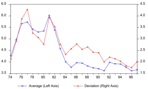
Figure 1 displays the average government capital expenditure - GDP ratio for a reduced sample of 19 developing countries6 over the period 1974-1997 (left hand side
scale) and the standard deviation (right hand side scale). The first remark is that, on average, the public investment ratios observed for these countries are very close to the values observed for OECD countries. The mean of the capital expenditure ratios in our sample is 4.42%. This value roughly corresponds to that observed on average for the OECD countries before the middle of the 1970s (Romp and De Haan, 2005). As it was stated for OECD countries (Ford and Poret, 1991; Sturm, 1998; Kamps, 2004), the average public investments - GDP ratio also decreases for the developing countries of our sample. The average ratio was 5.15% for the period 1974-1984, and only 3.80% after 1985. Two remarks can be made at this step. Firstly, the decline of public capital spending in the developing countries of our sample is, on average, comparable to the decline observed in the 1970s in the OECD countries. For instance, the public investment to GDP ratio for the United Sates was equal to 6.10% in 1961 and was only slightly superior to 3.00% in 1997. In France, this ratio was relatively stable, around 3.5%, for the period 1960-1990. However, in the same time the average part of the other public expenditures in the GDP increased from 40% during the period 1960-1979 to more than 50% during 1990-1997 (Hurlin, 2000). Secondly, this decline has occurred later in developing countries than in OECD countries. It seems that, on average, the decline in the ratios of government capital expenditure to GDP started after the beginning of the 1980s, and mainly occurred in this decade. This observation is identical to that made by Calderon, Easterly and Serven (2004) for nine Latin American economies where the decline was partly due to the context of fiscal austerity of the 1980s and 1990s. On the contrary, it is largely acknowledged that the decline of OECD public investments mainly occurred in the 1970s and even at the early beginning of 1970s for the United States if we consider infrastructure investments in roads (Fernald, 1999). Finally, it is important to remark that the average ratio reached at the end of 1990s in the developing countries of our sample, i.e. 3.70%, remains superior to the average ratio observed in OECD countries at the same period, i.e. around 3.00%.
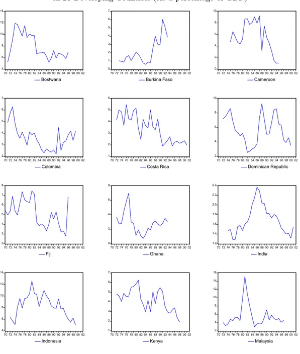
These conclusions based on average ratios hide a very heterogeneous reality. Figure 2 displays the government capital expenditure - GDP ratios for the 26 countries of our sample. This ratio varies considerably across countries. Over the period 1974-1997, the average ratio ranged from 1.73% for India to 9.26% for the Morocco. Moreover, the trends are very heterogeneous. For instance, the decrease in the public investment ratios is very pronounced during the 1980s for most of the Latin American countries of our sample (Mexico, Panama, Peru, and Venezuela), except Colombia and Paraguay where the decline mainly occurred during the 1970s. In the same time, the govern-ment capital expenditures are relatively stable in Thailand. This opposition between the Latin America and one of the East Asian Miracle Economies (World Bank, 1994)
6Since our panel is unbalanced, the average ratios displayed on Figure 1 are computed using a
reduced and balanced sample of 19 countries over the period 1974-1997. The excluded countries are the followings: Botswana, Burkina Faso, Cameroon, Fiji, Ghana, Mauritius and Zimbabwe.
reflects the oppositions observed by Calderon, Easterly and Serven (2004), when they consider physical measures of infrastructure. The only global and common observation that we can make at this step concerns the volatility of the public investment ratios. The variances of these ratios in the developing countries are clearly superior to those observed in the OECD countries. Using Kamps’s database (2004), Romp and De Haan (2005) found that the standard deviation of the government investment ratio for OECD 22 countries during the period 1960-2001 ranged from 1.00% to 1.80%. On the Figure 1, it can be observed that the corresponding standard deviation for developing countries during the period 1974-1997 ranges from 1.75% in 1996 to 4.28% in 1977. This high volatility is clearly observed on Figure 2 for the majority of the countries of our panel. This result is undoubtedly linked to the particular status of the public investments component in the total public expenditures. Much, although not all, of the public spending decline can be traced to fiscal adjustment. As it was earlier noted by Oxley and Martin (1991) ”the political reality is that it is easier to cut-back or post-pone investment spending than it is to cut current expenditures”. Consequently, the public investment is generally more reduced during times of fiscal stringency than the other public expenditures. This observation has been largely documented for OECD countries (Sturm, 1998), but also for Latin American countries (Calderon, Easterly and Serven, 2004) or for some African countries (World Bank, 1994). The developing countries, as other countries, lower their budget deficit mainly by cuts in capital spending. However, the amplitude of these adjustments and their frequencies seem to be more important in the developing countries.
As it was previously mentioned, two other elements are now required to estimate the net capital stocks: the time profile of the depreciation rate and an evaluation of the initial stocks.
2.2
Depreciation Profiles
In the PIM, the pattern of depreciation charges for a given assets is determined by its ”depreciation profile”. This profile describes the pattern of how, in the absence of inflation, the price of an asset declines as it ages. In this study, we consider a geometric pattern for the depreciation of public capital. For any given year, the constant-dollar depreciation charge is obtained by multiplying the depreciation charge in the preceding year by one minus the annual depreciation rate. It corresponds to the depreciation profile generally used in the literature devoted to the estimation of net capital stocks (private or public) and in particular used by the BEA for the United States to evaluate the majority of assets, including government assets (Bureau of Economic Analysis, 1999 and 2003.). This choice is also justified by the fact that the available data suggest that geometric patterns closely approximate the actual profile of price declines for a number of assets7 (Hulten and Wykoff, 1981). That is why, the geometric pattern was used to
measure the depreciation of public capital by Kamps (2004a,b) for OECD countries, Sturm and De Haan (1995) for the Netherlands, Berndt and Hansson (1992) for Sweden, Ford and Poret (1991) for France and Japan. The only exception is Declercq (1994)
7Hulten and Wykoff show that in a collection of assets, if each asset depreciates as an on-hoss shay,
who used physical measures and technical mortality tables to estimate the net capital stocks of infrastructure in France.
In this context, the issue is to choose the appropriate geometric depreciation rate and mainly to decide if this depreciation is constant over time. Given the level of aggregation of our public investments data, we decide to consider a time varying depre-ciation profile8 as it was done by Kamps (2004) for OECD countries or Declercq (1994) for France. The reason of our choice is the following: generally, for a given asset, the depreciation rate is assumed to be constant over time, except for some assets related to information and communication technology (BEA, 1999). However, the structure of public investments has deeply changed over the last decades. As the relative impor-tance of the different kinds of assets changes with time, so the average depreciation rate defined on the total stock does. Consequently, the depreciation rate of the aggregated stock cannot be assumed constant. For instance, Kamps (1994) shows that the average depreciation rate for public capital in the United States, approximated by an implicit scrapping rate defined as the quotient of total depreciation to the total net stock, has slowly increased during the period 1960-2001. He explains this increase by the increase of the proportion of the assets having relatively short lifetime comparing to all the other assets. Thus, the time varying depreciation profile of the aggregated stock of capital is directly related to the changes in the composition of public investments. These changes and their consequences on the public capital productivity have been largely studied for the United States (Gramlich, 1994; Cain, 1997; Fernald, 1999; etc.), mainly because sufficiently disaggregated data are available in the ”Fixed and Reproducible Tangible Wealth” BEA’s database. In this database, the total net stock of government capi-tal (Federal, State and Local) is divided in two parts, equipment and structures, and this last component represents roughly 85% of the total stocks. For the structures, the BEA distinguishes six broad categories9 of assets: Buildings (including residential,
industrial, educational, hospital and other), Highways and Streets, Military facilities, Conservation and Development, Sewer systems structures, Water supply facilities and Other structures. The most important categories during the period 1990-1996 are the buildings (including educational buildings) and the highways and streets (respectively around 30% and 26% of the total stocks). We can observe on Figure 3 that the part of these two main components in the total government net stocks has slowly decreased since the 1970’s. At the same time for instance, the part of the net capital stocks corre-sponding to water and sewer systems has increased. There are numerous reasons which could explain these modifications in the composition of the public capital stocks of the United States: the achievement of the great highways projects such as the Interstate Highway System (Fernald, 1999), the changes in the demography structure which have affected all the investments related to education (Sturm, 1998) or more originally, the legal constraints or the federal subvention10 (Hulten and Schwab, 1997).
8Kamps (2004) and Declerq (1994) are the only examples of the use of a time varying depreciation
profile for public capital stocks.
9More precise sub-categories are also available. 1 0
Hulten and Schwab (1997) point out the influence of the Federal Water Pollution Act (1972) and the Clean Water Act (1977) on the amount of subventions devoted to the water and sewer systems investments.
To the best of our knowledge, there is no similar study devoted to the composition of public capital stocks in developing countries or even in the major OECD countries except the United States. However, it is reasonable to assume that, in developing countries, the structure of public capital stocks has changed over the last decades, even if these changes are not similar to those observed for the United States. This evolution of stocks can be pointed out using the evolution of the composition of investments. There are few studies devoted to the structure of public investments in developing countries over long period of time. One exception is the recent study proposed by Calderon, Easterly and Serven (2004) for nine Latin American countries11 over 1980-1998. Their decomposition is based on six broad categories: road, railways, electricity, gas, water and telecoms. On Figure 4, the average proportions of these categories in the total public investments for these nine countries are reported. Even if this structure of investments cannot be directly compared to the structure of the net stocks of United States, we still can observe some important differences. For instance, the proportion of investments in roads in LA increased during the 1980’s, while we observe a decrease of the part of this kind of investments in US during the same period (Fernald, 1999). The part of investments in railways and electricity in LA decreased quickly at the end of 1980’s and the early of 1990’s due to privatisations (Calderon, Easterly and Serven, 2004) and naturally we do not have the same evolution for the US investments during the same period. These observations confirm our conviction that we cannot use the structure of public investments / stocks in US or other OECD countries as a proxy for the developing countries. Consequently, it implies that it is not reliable to use the same time profile of depreciation for developing countries as for OECD countries since this time profile is directly related to the composition of stocks. For these reasons, we propose to estimate a time profile of depreciation rates specific to developing countries12 and based on the changes of the composition of public investments observed in LA.
In order to estimate a time profile of the depreciation rates for the aggregated capital specific to developing countries, we propose the following definition. The time varying depreciation rate is defined as a weighted average of the constant depreciation rates of the six components of public investments defined in Calderon, Easterly and Serven (2004). This estimate requires two inputs: constant depreciation rates for the six types of assets used in the decomposition and the weights of these assets in the total stocks. For the first input, we propose to use the BEA depreciations rates. This is appropriate insofar as country-specific factors influence service lifetime. In particular, recurrent infrastructure expenditures for operation and maintenance are generally cut along with investments, and this decline may accelerate the depreciation of stocks. However, we do not have information about the potential reduction of the service lifetime of public investments in developing countries. Moreover, the literature devoted to public capital stocks does not assert that services lifetime of equipments or structures is shorter in developing countries than in other countries. The main particularity raised in the case
1 1These countries are: Argentina, Bolivia, Brazil, Chile, Colombia, Ecuador, Mexico, Peru,
Venezuela, R.B. de.
1 2
So we will assume that the time profile is the same accross countries, as it was done in Kamsp (2004) or Maddison (1995).
of developing countries is that public investments may not create productive capital (Pritchett, 1996) and not that the depreciation of stocks is more accelerated.
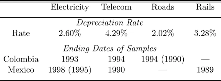
The BEA computes net capital stocks from a detailed division of assets (Bureau of Economic Analysis, 1999, tables C). Ideally, depreciation profiles should be based on empirical evidence on used asset prices in resale markets. Such an evaluation is possible only for some assets (autos, computers for instance). In this case, the profile can be estimated using prices in the corresponding resale market. For all other assets, geo-metric profiles are used. For a given type of asset, the estimated rate of depreciation is derived from the estimates of Hulten and Wykoff (1979, 1981). The depreciation rate is determined by dividing the declining-balance rate13 by the corresponding as-sumed service life expressed in years. Hulten and Wykoff obtained that, on average, the declining-balance rate for producer’s durable equipment was 1.65 and that for non-residential structures was 0.91. Given the BEA classification, we choose the assets that are the closest to the decomposition of investments proposed by Calderon, Easterly and Serven (2004). The geometric depreciation rates, the underlying declining-balance depreciation rates and the services lives used by BEA for these assets are reported in Table 1. For each type of investment two depreciation rates are proposed by the BEA: one for equipment and one for structures. The only exceptions are the investments in roads, gas and water systems for which only structure assets are reported. Taking into account these information, we compute a weighted average of the rates on struc-tures and equipment for all the six components of public investments used in Calderon, Easterly and Serven (2004). The weights are defined by the average part of equipment assets (respectively structure assets) in the total government net stocks of the United States over the period 1950-1996. The weights used are then defined by 83.17% for structures and 16.83% for equipments. The corresponding depreciation rates used for the six components of public investments are reported in Table 2. The mean of these depreciations rates is equal to 2.68% which is roughly the same value used by Kamps in his study of OECD countries until the 1970’s. Logically, the lowest values of deprecia-tion rates are obtained for roads and water systems and the highest value corresponds to the telecommunication sector where the service lifetime of assets is the shorter.
The second input required to estimate the depreciation rate for the aggregated stocks is the weight of each type of assets in the total stocks. Let us consider the general case with m types of assets. For each asset, the capital stock at the beginning of period t is denoted Ki t, with i = 1, .., m and t = 1, ..T. The corresponding depreciation rate,
denoted δi, is assumed to be constant over time. If we consider a perpetual inventory
method, and if we note Ii,tthe gross investment in the ith asset for the current period,
we have:
Ki,t+1= (1 − δi) Kit+ Iit i = 1, .., m (1)
Then, the process which generates the total stocks eKt=Pmi=1Kit is defined as:
e Kt+1 = m X i=1 (1 − δi) Kit+ eIt (2) 1 3The declining balance rate is equal to the multiple of the comparable straight-line rate.
where eIt =Pmi=1Iit denotes the total investments. This process of accumulation can
be rewritten using a the time varying depreciation rate, denoted eδt, as:
e Kt+1= ³ 1 − eδt ´ e Kt+ eIt
Identifying equations (1) and (2), it is possible to derive the aggregated depreciation time profile by the variable as a weighted average of constant specific depreciation rates. In this case, the weights, denoted Wit, are defined by the proportion of the capital stocks
Kit in the total stocks eKtat time t.
eδt= m X i=1 δiWit= m X i=1 δi Kit e Kt (3)
However, we do not have some information about the ratios Kit/ eKt since there
are no available data on sectoral public capital stocks. A solution would consist in approximating the weights Wit by the ratio of investments Iit/eIt. In this case, the time
profile of the depreciation rates would be estimated by:
eδt' eδ ∗ t = m X i=1 δi Iit e It (4)
The sequence of estimated depreciation rates eδ∗t based on this approximation over the period 1980-1998 is reported on Figure 5. The ratios Iit/eIt are computed using
the data of Calderon, Easterly and Serven (2004) for the following six components of investments: road, railways, electricity, gas, water and telecoms. The constant depreciation rates δi, i = 1, ..6, correspond to the values reported in Table 2. We can
observe that the estimated depreciation time profile slowly decreased from 2.74% in 1980 to 2.38% in 1998. This decrease mainly occurred after the end of 1980’s. This stability of the depreciation rates in the 1980’s (between 2.75% and 2.80%) and the slight decrease in the 1990’s is clearly visible when the depreciation rates are smoothed. Figure 5 displays the depreciation rates smoothed by a simple Hodrick and Prescott (1980) filter. Two values of the smoothing parameter recommended for annual data are used in order to assess the robustness of our results: the standard value of 100 proposed notably by Backus and Kehoe (1992), but also a value of 6.25 recommended by Ravn and Uhlig (2002). Using these parameters, the smoothed time profiles of depreciation are similar. The smoothed depreciation rate ranges from 2.77% in 1980 to 2.50% in 1998 and we can distinguish two periods: a period of stability in the 1980’s and a period of decrease in the 1990’s. Similar conclusions (see Figure 1 in Appendix B.1) are obtained if we use a local regression on time (or Loess regression, Cleveland and Devlin, 1988) with an optimal smoothing parameter chosen according to a modified AIC criterion.
This slight decrease of the depreciation rates is in opposition to the depreciation profile observed by Kamps (2004) for OCDE countries after 1960. Indeed, Kamps (2004) determines the depreciation profile for the OECD countries by approximating an implicit scrapping rate calculated for the United States over the period 1960-2000.
He finds that this scrapping rate has tended to rise over time. Consequently he assumes a constant depreciation rate of 2,50% for the period 1860 to 1960, and an increasing rate for the period 1960-2001. During this last period, the depreciation rates for OECD countries are assumed to increase gradually from 2.50% to 4.00%. He explains this in-crease of depreciation rates by the increasing weight of short lifetime assets. However, considering the Calderon, Easterly and Serven (2004) decomposition in LA countries since the 1980’s, we observe an increasing weight of assets with relatively long service lifetime, as roads and water systems (Figure 4). That is why we found that the ag-gregated depreciation rates for developing countries had decreased. This result does not exclude the possibility of an increase in the next decades due, for instance, to the investments in information and communication technologies. At the same time, our results could be interpreted as an increase in the assets lifetime imposed by a lack of replacement investments.
One of the major drawbacks of this first approximation comes from the fact that the weights are defined by the ratios of investments. These ratios reflect the composition of new equipments or structures, and not the composition of the stock determined by the past investments. That is why, we propose a second approximation of the weights used in the definition (3) of the aggregated depreciation rates. Let us consider a perpetual inventory method for each asset (equation 1) . For t ≥ 2, we have:
Kit = t−2
X
h=0
(1 − δi)hIi,t−1−h+ (1 − δi)t−1 Ki1 (5)
where Ki1 denotes the initial stock for the asset i. Let us denote eKt = Pmi=1Kit the
total stock at the beginning of the period t. Then, the weight Wi,t of the ith asset at
time t in aggregated depreciation rate is defined as:
Wit = "t−2 X h=0 (1 − δi)hIi,t−1−h+ (1 − δi)t−1 Ki1 # × "m X i=1 t−2 X h=0 (1 − δi)hIi,t−1−h+ m X i=1 (1 − δi)t−1 Ki1 #−1 (6)
Naturally, in this expression the initial conditions {Ki1}mi=1 are unknown. Let us
denote βi the ratios of initial value Ki1 to the initial total stock eK1 and α the ratio of
total public investments to the total public capital stock at the first period, α = eI1/ eK1.
The weights Wit can be rewritten as:
Wit(β, α) = "t−2 X h=0 (1 − δi)hIi,t−1−h+ µ βi α ¶ (1 − δi)t−1Ie1 # × "m X i=1 t−2 X h=0 (1 − δi)hIi,t−1−h+ Ã e I1 α ! m X i=1 βi(1 − δi)t−1 #−1 (7)
with β = (β1, ..βm) . The ratio α of public investment to public capital stock is cali-brated to the average value observed14 for the United States over the period 1950-1996,
i.e. 0, 0573. A sensitivity analysis to the value of this parameter will be proposed with five values of the parameter α = {0.01; 0.04; 0.05; 0.06; 0.10}. Like the previous approximation, the public investments Iitare taken from the data of Calderon, Easterly
and Serven (2004) with m = 6 components of investments. The constant depreciation rates δi are taken from Table 2. Finally, the ratios of the initial values of stocks βi
are calibrated15 to the mean of the corresponding ratios of investments over the period
1980-1998 for the considered LA countries.
The sequence of the corrected depreciation rates eδct = Pmi=1δiWit(α, β) based on
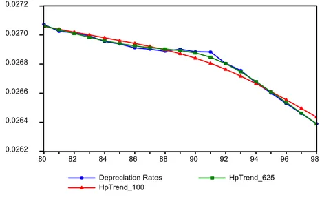
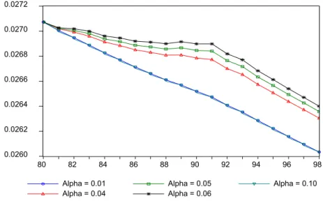
this approximation is reported on Figure 6. For the benchmark values of parameter α and β, the decrease of the depreciation rates is confirmed. However, this decrease is less important than the decrease observed with the previous approximation. The depreciation rate ranges from 2.639% in 1998 to 2.707% in 1980. Logically, the profile of depreciation is smoother than the previous profile computed with ratios of invest-ments. Consequently, whatever the value of the smoothing parameter, the HP trend components are similar to the series of estimated depreciations rates. The results are similar when we consider different values of the ratio α of public investments to public capital stock at the first period. A sensitivity analysis of our results to the values of α = {0.01; 0.04; 0.05; 0.06; 0.10} is reported on the Figure 7. Given these results, we propose to use our estimated series eδct and eδ∗t as benchmark depreciation rates for the developing countries of our sample. More precisely, we consider the smoothed values of these depreciation rates obtained by a local regression (LOESS) over time (see Ap-pendix A.1). We prefer this smoothing method to the HP filter, since it is well known that the HP filter has not good properties at the extreme points of the sample. For the period before 1980, we assume that the depreciation is constant: its value is fixed to the first estimated value for 1980, i.e. 2, 71% for the corrected depreciation rate eδct and 2, 77% for the non corrected depreciation rate eδ∗t. The corresponding depreciation time profiles are displayed on Figure 8 and the values are reported in Table A3 (Appendix B.2). In a next section, we will analyze the sensitivity of our net capital stock estimates to the depreciation pattern used. Moreover, apart from these quantitative results, we are convinced that the use of a slight decreasing (or at the most constant) depreciation time profile for developing countries is justified for the arguments mentioned above. Given the decomposition of investments observed by Calderon, Easterly and Serven (2004) for LA countries over the period 1980-1998, we think that the increasing de-preciation time profile used for OECD countries could not be used as a benchmark for developing countries.
1 4A similar value of 0.0666 is founded if we consider that in average the ratio of public capital stocks
to GDP is near to 0.60 and the ratio of public investments to GDP is near to 0.04, as it is observed for OECD countries
1 5
These values, expressed as a percentage, are the followings. Road: β1 = 14.70, Railways: β2 =
9.60, Electricity: β3= 46.27,Gas: β4= 0.53,Water: β5= 12.97,Telecoms: β6= 15.89.A analysis of
sensitivity was done with βi= 1/6for all assets results to the same qualitative depreciation profile for
all the considered values of α. The maximum value of the depreciation rate was then 2.68% and the minimum achieved in 1998 was around 2.56%.
2.3
Initial Stocks
The second input required in the application of the perpetual inventory method is the initial public capital stock. When no information about the initial value of the capital stock is available, one of the possible solutions consists in assuming a null initial stock. However, in order to limit the consequences of this assumption, we will consider the same assumptions as those used by Jacob, Sharma and Grawbowski (1997) or Kamps (2004) for OECD countries. For each country of our panel, an artificial investment series is constructed since 1880 by assuming that investment increased by 4 percent per year and finally reaching its observed level at the first date of our sample. This series is used as input to estimate the initial capital stock for each country. The stock in 1880 is set equal to zero and the depreciation rate used corresponds to the first value of our estimated series eδct, i.e. 2.71%. We will analyze in the next section the sensitivity of our net capital stocks to the choice of initial stock, but we need to remind here that this influence decreases over time. Indeed, for a time-varying depreciation rate δt, the
net public capital stock at time t, denoted Kt, is defined as:
Kt+1= t−1 X h=0 "h−1 Y z=0 (1 − δt−z) # It−h+ t−1 Y z=0 (1 − δt−z) K1 (8)
where Ki1 denotes the initial stock and where δt < 1. Consequently, an error on the
value of the initial net capital stock has therefore only a temporary effect.
To sum up, in order to estimate our benchmark net capital stocks by the perpet-ual inventory method, we made two main assumptions. The first concerns the initial capital stock. This initial value of the net capital stock is constructed from an artifi-cial investment series which starts in 1880. The second main assumption concerns the depreciation pattern. As it was generally the case, we choose a geometric depreciation pattern. But, we also use a time varying depreciation rate profile, with a slight decrease after the beginning of the 1980’s. This decrease reflects the changes in the composition of the public investments observed for the LA countries and considered as a benchmark for our sample of developing countries.
2.4
Net Capital Stock Estimates for Developing Countries
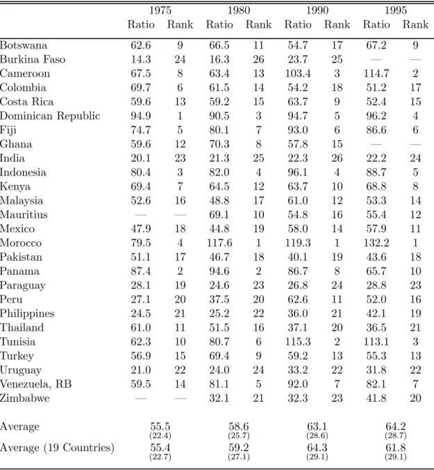
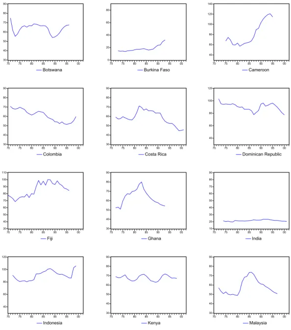
Figure 9 displays the evolution of the ratio of the public net capital stock to GDP for the 26 countries of our panel. The capital stock estimates are expressed in national currency and valued with national constant prices16. Logically, we found similar conclusions as those raised for the public investments in the previous section. In order to compare our benchmark results with those of Kamps (2004a) for OECD countries, the values of the public capital GDP ratio for four reference years (1975, 1980, 1990 and 1995) are also displayed in Table 3. The main difference is that we observe an increase of the average net capital stock ratio for our panel of developing countries, while Kamps observes a decline of the corresponding ratio for OECD countries. In our sample, the average ratio increases from 58.6% in 1980 to 63.1% in 1990. When we consider
1 6
The base year is not the same for all countries and corresponds to the base year used for the GDP deflator. The GDP used is alos expressed in constant prices, WDI code: NY.GDP.MKTP.KN.
a balanced panel of 19 countries17, the corresponding values are 59.2% and 64.3%. During the same period, the estimated ratios for 22 OECD countries decreased from 57.8% to 55.3% (Kamps 2004, Table 2, page 28). At least two factors could explain this evolution: the first is the depreciation pattern18, the second and most important is the delay in the decline of public investments in developing countries. As it was previously mentioned, in our sample the average ratio of public investments to GDP has declined only after the middle of the 1980s, while in the most of OECD countries this evolution has occurred in the 1970s. Consequently, the corresponding decrease in the stock ratios is logically delayed in our sample. More precisely, we do no observe a decrease as in the OECD countries, but only a drastic decrease in the growth of the capital to GDP ratio: this ratio increased from 55.5% to 58.6% from 1975 to 1980, but only from 63.1% to 64.2% from 1990 to 1995. If we consider the balanced panel of 19 countries, we observe a decrease as severe as that reported by Kamps, since the ratio declined from 64.3% in 1990 to 61.8% in 1995. In other words, the PIM approach allows us to date the deceleration of the growth of the public capital stock, on average, at the beginning of the 1990s, i.e. at least two decades after the deceleration observed in the United States (Fernald, 1999). Moreover, at the end of the 1990s, the average capital to GDP ratio in developing countries remained similar, or even superior, to that observed in OECD countries. However, given the drawbacks of the use of the PIM for the case of developing countries this conclusion cannot be interpreted as the diagnostic that, relatively to their GDP, many developing countries have no shortages of public investments or capital stocks. Our estimates only allow us to point out the deceleration of the public capital stock growth in 1990s, at least one decade after the same phenomenon was observed in the OECD countries. This evolution can be viewed as a consequence of the fiscal adjustments (but this is not the only factor) implemented in the 1980s. Except if we assume that the efficiency of public investments in creating public capital dramatically changed over the period 1975 -1995, these observations based on the PIM remain valid if we consider the true part of public investments really productive in creating public capital. Nothing allows us to think that any global improvement in the efficiency of public investments would compensate the decrease of the ratio of public capital stocks to GDP during the 1990s. Finally, as pointed out by Kamps (2004a), the main advantage of these benchmark estimates is that they rely on the same methodology and on homogenous investment data across countries.
These global evolutions hide heterogeneous trends among the countries of our sam-ple. Between 1975 and 1980, public capital expressed as part of GDP has increased in 14 countries out of 24. Between 1990 and 1995, this ratio increased only for 10 countries. However, despite these evolutions, there exists a relative stability of the group of countries with the highest ratios of public capital. If we compare the ranking according this ratio in 1975 and in 1995, 9 countries are always among the 10 highest ratios (Table 3). These countries are Botswana, Cameroon, Dominican Republic, Fiji,
1 7
Excluded countries are: Botswana, Burkina Faso, Cameroon, Fiji, Ghana, Mauritius and Zim-babwe.
1 8For a given GDP, the decrease of the depreciation rate induces an increase of the capital stock to
GDP ratio. However, the depreciation pattern does not explain a substantial part of the evolution of our capital stock estimates, as we will see in the section devoted to the robustness of our estimates.
Indonesia, Kenya, Morocco, Panama and Tunisia. Only Colombia has been excluded from this group between 1975 and 1995 and has been replaced by the Venezuela. And, since the Colombia witnessed an infrastructure investment expansion during the late 1990s, this evolution would not be observed if the reference was taking at the early of 2000s. Thus, these benchmark estimates based on the PIM show a relative stability of the ranking of the countries according to their ratio of public capital stocks to GDP. Naturally, the robustness of theses estimates must be evaluated.
2.5
Robustness of the Public Capital Stock Estimates
The drawbacks of the perpetual inventory method are well known. The largest one is that the use of the PIM requires a variety of assumptions concerning depreciation patterns and the treatment of an initial stock. That is why we now propose to evaluate the robustness of our public capital stock estimates to these assumptions as it was done by Kamps (2004a). For this purpose we will consider four reference countries: Pakistan, Peru, Philippines and Tunisia. For each assumption used in this section, we will estimates new net capital stocks series for these four countries. These series will be compared with our benchmark PIM estimates from the point of view of the levels but also from the point of view of growth rates.
Concerning the depreciation patterns, two assumptions are made: the first is the geometric pattern and the second assumption is the use of a time varying depreciation rate. Firstly, let us consider the influence of time profile of the depreciation rates on our estimates. As it was shown in the previous section, our aggregated depreciation rates are estimated using the composition of public investments in LA as a benchmark for all the developing countries of our sample. Using this method, we found a slight decreasing time profile reflecting the decline of the part of public investments in assets having short life services. The influence of these assumptions on our final estimates must be evaluated. For that, for each reference country two other capital stocks are estimated with two alternative assumptions on the depreciation time profile. For the first estimate we consider a constant annual depreciation rate of 4.0% over the period 1970-20002. If we admit that on average the declining-balance rate for equipment is 1.65 and 0.91 for non residential structures, it corresponds to a service lifetime of 41.25 years and respectively 22.75 years. This values of the depreciation rate is largely superior to the values considered in our benchmark estimates which range from 2.64% to 2.71%. For the second estimate, we assume that the depreciation time profile for developing countries is exactly the same as that estimated by Kamps (2004a) for OECD country. The author assumes that the depreciation rate gradually increased from 2.50% to 4% over the period 1960-2001 according to the following formula:
δt= ( 2.50% ∀t < 1960 0.0250h¡0.0250.04¢ 1 41 it−2001+41 ∀t ≥ 1960 (9)
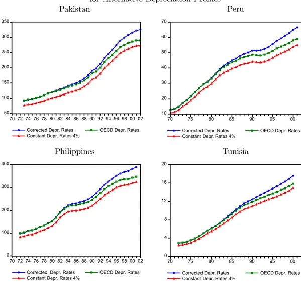
Figure 10 displays the estimates of net public capital stock, expressed in local cur-rency unit at constant prices, for the alternative assumptions on the depreciation time profile. Logically, the net stocks evaluated with the constant depreciation rate of 4.00%
are always inferior to our benchmark estimates, but both dynamics are quite similar as we can observe on Figure 11 where the corresponding growth rates are displayed. This result is logical since our benchmark depreciation rates do not vary before 1980 and are only slightly decreasing after this date. Then, the corresponding dynamics of our estimates is quite similar to that obtained with a constant depreciation rate. The stocks evaluated with the depreciation rates used by Kamps (2004a) are also quite similar to our benchmark estimates at the early of the 1970s. Indeed, given the formula used by Kamps, the aggregated depreciation rate for OECD countries is equal to 2.80% in 1970, while our benchmark estimated depreciation rate at the same date is 2.71%. But in this case, the difference between both depreciation rates has increased over time. That is why the difference between the corresponding estimated stocks has also increased over time. In 2000, the difference between both estimated stocks reached 9.31% of the benchmark stock for Pakistan, 10.65% for Peru, 10.19% for Philippines and 9.85% for Tunisia. Given the potential sources of errors due to the perpetual inventory method in the valuation of the estimates of capital stocks, such a difference can be considered as negligible. Secondly, as mentioned above, the use of a geometric pattern is very general in the literature devoted to the net capital stock estimates, and not only for public capital stocks. Besides, Hulten and Wyckoff (1981) show that if different capital goods are lumped together, the geometric depreciation rate gives a reasonable statis-tical approximation of the true depreciation rate. For these reasons, we do not report the sensitivity analysis of our estimates to other methods of depreciation (straight-line, hyperbolic etc.). Kamps reports the results of this type of sensitivity analysis for his net public capital stock estimates for OECD countries. He shows that hyperbolic and geometric depreciation result in quite similar capital stock estimates whereas the estimates based on straight-line depreciation differ considerably in levels and also in dynamics.
Finally, we propose an evaluation of the robustness of our estimates to the choice of the initial condition. Naturally, the estimation of the initial capital stocks, which consist in accumulated past investments, presents substantial problems, since no in-formation is available about public investments over long period of time, even for the OECD countries. In our study, the benchmark estimates are computed with an initial stock defined as the accumulation of a pseudo public investment series. This approach requires several assumptions: (1) an averaged growth rate for the pseudo investment series (2) an initial condition for the stock or equivalently a starting date for the pseudo series and (3) a depreciation rate over this period. As it was explained in the previous section, we consider an averaged growth rate of investments equal to 4.00% for all the countries of our sample, a depreciation rate equal to 2.71% and a starting date in 1880, i.e. twenty years after the initial date considered by Kamps for OECD countries. In order to determine the sensitivity of our estimates to these assumptions, we consider two alternative sets of assumptions. In the first set, we assume that the pseudo series starts in 1920. Consequently, this assumption implies a lower initial stock for all the countries of the panel. In the second set of assumptions, the starting date remains unchanged, but we consider a heterogeneous growth rate of investments to compute the pseudo investment series. For each country, the growth rate used is set equal to the historical growth observed over the period 1970-2000. Figures 12 and 13 display the
corresponding estimates of the net capital stocks and the growth rates of net capital stocks. For three reference countries (Pakistan, Philippines and Tunisia) the use of the national growth rate of public investment to build the pseudo series of past investments leads to an initial capital stock higher than the benchmark ones. In these cases, the difference between the two initial stocks expressed as percentage of the benchmark ini-tial stock ranges from 20.9% for Philippines to −29.62% for Tunisia. However these important differences rapidly decrease with time. At the end of the sample, the dif-ference between the estimates of capital stocks is 1.17% for Pakistan, 0.70% for Peru, 2.39% for Philippines and -2.41% for Tunisia. Besides, the dynamics of growth rates of capital stocks are quite similar under various assumptions concerning the time profile of depreciation rates.
These observations show that, at least for these reference countries, the dynamics of our benchmark PIM estimates of net public capital stocks are relatively robust to some changes in the time depreciation profile or in the value of the initial stocks. Moreover, it is obvious that if the public capital stocks in developing countries were overvalued, it would be due rather to a mis-measurement of the part of monetary investments which were really transformed in productive capital rather than due to a mis-measurement of the depreciation rates or of the initial stocks.
3
Public Investment and Efficiency
The main drawbacks of the PIM method are well known. The two largest are the fact that this estimation method requires a variety of assumptions concerning service lives and depreciation patterns and an evaluation of initial stock. Firstly, we have proposed a sensitivity analysis of our estimates to these assumptions, and secondly these drawbacks are not specific to the developing countries. For both reasons, the net capital stocks estimated by the PIM can be used to compare the productivity of public capital in developing countries and in OECD countries. However, there is another problem considered as more specific19 to developing countries: it is the efficiency of public investments in creating capital.
Indeed, Summers and Heston (1991), Pritchett (1996) or Canning (1998) state that the same investment flows in different countries may have very different effectiveness in actually producing capital, due to the differences in the efficiency of the public sector and differences in the price of capital. If the investment project is carried out by the public sector, actual and economic costs (defined as the minimum of possible costs given available technology) may deviate. So, monetary investment in infrastructure may be a very poor proxy of the amount of public capital actually produced. For instance, Pritchett suggests that in a typical developing country less than 50 cents of capital were created for each public dollar invested. He concludes that ”one of the deep difficulties of development may well be that even when public capital is productive it
1 9
We assert that this issue is specific to developing countries since only studies devoted to these countries evoked this problem. To the best of our knowledge, in the huge litterature devoted to the public capital in the United States, there is no study that points out this fact. But, this is not a proof of the specificity that the inefficiency of public investments is specific in developing countries.
may be difficult to create this capital in the public sector ” (Pritchett, 1996, page 1). Given this potential inefficiency of public investments, the use of monetary investment flows may introduce systematic errors in stock estimates. In particular, it implies that public capital stock series constructed with the PIM will tend to be overvalued.
In this section, we firstly intend to evaluate this inefficiency using an original methodology and secondly to estimate net stocks only based on the productive compo-nent of investments.
3.1
Public Investment Efficiency: a Non Parametric Approach
The idea that a dollar’s worth of public investment spending often does not create a dollar’s worth of capital can be expressed as follows:
Kt+1= (1 − δ) Kt+ f (It) (10)
where Ktdenotes the real public capital stock at time t and I denotes the corresponding
gross public investment. The function f (It) represents the efficiency of public
invest-ments to generate new capital. We assume that efficiency is constant over time, i.e. the function f (.) does not vary with time. Since the relative efficiency may vary with the amount of investments, such an assumption is not very restrictive. The perpetual inventory method assumes that this function is always defined as the identity function:
f (It) = It (11)
On the contrary if we assume that, according to Pritchett (1996), in a typical developing countries only a certain part of investments is used to create the public capital, the function f (.) satisfies the following constraints:
0 ≤ f (It) < It (12)
f (0) = 0 (13)
The fact that f (It) is strictly inferior to Itreflects the inefficiency of public investments
in creating capital. The more different from zero is the distance |f (It) − It| , the less
appropriate to estimate public capital stocks is the PIM method. If this efficiency function were known, it would be possible to estimate the ”productive” component of investments at each date and consequently to estimate the genuine net public capital stocks by the PIM, as presented in the previous section. It is important to note that it is not the PIM itself which is a problem for the developing countries. It is the fact that the PIM is based on the total monetary flows of gross investments which is problematic.
In this context, the main issue is that it is very difficult to find a functional form for this function f (.). The simplest way would be to assume that productive investments are strictly proportional to the total investments. If, as it stated by Pritchett, less than 50 cents of capital were created for each public dollar invested, we would have:
with α < 1/2. The main drawback of this specification, is that we assume that the relative efficiency of public investments is constant in the amount of the investments. It implies that a huge spending going to white elephant has relatively the same efficiency (or inefficiency) as a little project of infrastructure for which the control can be stricter and more direct. Since no natural specification of the efficiency function f (.) can be justified a priori, another solution consists in estimating this function by a non parametric method for a country or for a sub-group of developing countries and in taking this estimate as a benchmark for all the countries of our sample. More precisely, the aim of our non parametric approach is not to evaluate the relative efficiency of public investments in the 26 countries of our panel, but to estimate the efficiency function for a sub-group of countries and to consider this estimated functional form (and not the corresponding efficiency) as benchmark for all the countries. For this purpose, three ingredients are required: (1) a series a public investments (2) the depreciation rates (or its time profile) and (3) a series of public capital net stocks effectively available in the reference countries. The last element is the most difficult to find. Indeed, in order to precisely estimate the public capital stock in developing countries, the efficiency function is required, and in order to estimate this function it is necessary to have the series of public capital.
In this study, we propose to estimate the efficiency function of the public invest-ments using the physical measure of infrastructure as a proxy20 of the public capital stock effectively used in the developing countries. Recently, in order to study the link between the public infrastructure spending and the physical infrastructure stocks, Calderon, Easterly and Serven (2004) used the same approximation21 for the Latin American countries. They used an ARDL specification with the sectoral monetary investments flows (for instance, the investments in the road sector) and the physical measures of the corresponding infrastructure, expressed as growth rate (for instance, the number of kilometers of paved road). Their regressions in panel models with or without fixed effects point out the statistical link between the past investment fluctu-ations and infrastructure level. ”The conclusion from these empirical experiments is that infrastructure investment is a robust predictor of subsequent changes in the physical infrastructure stock across countries and over time”. (Calderon, Easterly and Serven, page 62).
Here, our approach is different. Firstly, we do not intend to estimate a long term multiplier between the past investments and the variation of the physical infrastructure stocks in an ARDL specification. We intend to estimate the functional form f (.), which may be not linear, between the current monetary investments and the monetary variation of the current stock i.e.. Kt+1−(1 − δ) Kt. Secondly, our study is only devoted
to the link between the public investments and the public capital. On the contrary Calderon, Easterly and Serven analyze simultaneously the total private investments,
2 0
This idea which consists to estimate the efficiency function by comparing the variations of the physical measures of the capital to the monetary investments flows has been evoked by Pritchett (footnote 31, page 36, Pritchett 1996), when he considered the first data collected by Canning and Fay (1995) on the physical measures of the transport infrastructure.
2 1
the private investments and the public investments. Consequently, in order to estimate the link between the public investments and the public capital using physical measures, it is required to consider countries (1) for which there are available data about sectoral public investments over a long enough period of time, and (2) for which the private investments in the reference sectors are negligible comparing to the public investments. To the best of our knowledge, only the Calderon, Easterly and Serven’s database about nine countries of the Latin America allow an enough detailed decomposition of the public investments for a long period of time that allows us to establish a correspondence with the physical measures of the Caning’s database. That is why we choose two reference LA countries from our panel, Colombia and Mexico. For these two countries we compare the investments flows to the physical measure variations over the period 1981-1995. We use a decomposition of investments in four sectors for which there exist corresponding physical measures in the Caning’s database. These sectors are the following: electricity, telecommunication, roads and railways.
One of the problems of this decomposition is that it considers sectors for which private investments may be important. As in the majority of Latin America countries, in these two reference countries, the proportion private investments versus public of the investments in infrastructure deeply changed during the period 1981-1995. In order to avoid this problem, we consider only a period of time for which the part of private investments in the total investments is insignificant. More precisely, for each sector, the sample used for estimation starts in 1981 and ends at the dates reported in the Table 4. These ending dates have been chosen such that during the considered period of time, the amount of the private investments in the total investments of the specified sectors never exceeds 15%. So during these period, we can use the infrastructure as a proxy of the public capital for the considered sector. Generally, these dates correspond to the reform dates pointed out by Calderon, Easterly and Serven (2004).
The second problem concerning this sectoral decomposition is the correspondence between the investments categories and the infrastructure physical measures proposed by Canning. To measure the stock of infrastructure in the electricity sector we consider the electricity-generating capacity expressed in million of kilowatts. For the telecom-munication sector, two types of measures can be used: the number of telephone lines or the number of telephone main lines. We decide to use the second measure, which was notably considered in the ARDL specification estimated by Calderon, Easterly and Serven (2004). Two measures are also possible for the roads sector: the number of road kilometers or the number of paved road kilometers. For this sector, we decide to use the measure which allows us to cover better the estimation period for each country. Thus, for Mexico we use the number of road kilometers while for Colombia we use the number of paved road kilometers. Finally, to measure the investments in the railways sector, the number of the rail kilometers was used.
Then, the problem consists in estimating the functional form of the public invest-ments efficiency function. This function relates on the one hand the monetary flows of investments expressed in million US dollars and on the other hand the public capital stocks measured of in the same monetary unit. But, we have only physical measures of these stocks. Our methodology is then the following. Let us assume that at a certain