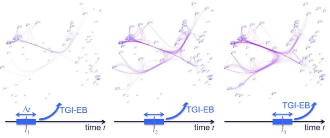
Bundling : une technique de réduction d'occultation par agrégation visuelle et son application à l'étude de la maladie d'Alzheimer

(1)

THÈSE

En vue de l’obtention du

DOCTORAT DE L’UNIVERSITÉ DE TOULOUSE

Délivré par : l’Université Toulouse 3 Paul Sabatier (UT3 Paul Sabatier)

Présentée et soutenue le 8/12/2017 par :

Antoine Lhuillier

Bundling : une Technique de Réduction d’Occultation par Agrégation Visuelle et son Application à l’Étude de la Maladie d’Alzheimer

JURY

David AUBER Maître de conférences Rapporteur

Daniel WEISKOPF Professeur d’université Rapporteur

Denis KOUAME Professeur d’université Président du jury

Caroline APPERT Chargé de recherche Membre du jury

Jean-Daniel FEKETE Directeur de recherche Membre du jury

Emmanuel BARBEAU Directeur de recherche Invité

Christophe HURTER Professeur Directeur de thèse

Christophe JOUFFRAIS Directeur de recherche Co-directeur de thèse

École doctorale et spécialité :

MITT : Image, Information, Hypermédia Unité de Recherche :

UR Laboratoire de recherche ENAC Directeur(s) de Thèse :

Christophe HURTER et Christophe JOUFFRAIS Rapporteurs :

(2)

(3)

i

Acknowledgements

First, I would like to deeply thank my PhD advisor Christophe Hurter who en-couraged me to pursue a PhD research. Thanks to his immense energy, patience and teaching skills he gave me the motivation and the keys to the scientific research. I could never have imagined any better supervisor, always present in the good as well as the more difficult times of my PhD.

I also would like to thanks all the members of this research project : Christophe Jouffrais, Emmanuel Barbeau and Hélène Amieva, without whom nothing would have been possible. Your various domain of expertise showed me the vast diversity of research and gave me insightful advices and invaluable interdisciplinary experience throughout my PhD. Furthermore, I would like also to acknowledge the support of the Federal University of Toulouse (Université Fédérale Toulouse Midi-Pyrénées - UFT-MiP) and the French Civil Aviation University (ENAC) who funded this project.

I thank very much the reviewers of my thesis David Auber and Daniel Weiskopf as well as all the members of my jury : Denis Kouamé, Caroline Appert and Jean-Daniel Fekete for their critiques, their feedbacks and ultimately for coming to my defence.

Then, I would like to warmly thank Alexandru Telea who helped me refine and challenge my work on bundling by bringing an external perspective during a difficult time of my PhD. I want to thank Ludovic Gardy for his work and help during my work on Alzheimer’s disease. I also thank the other PhD students : Almoctar Hassoumi, Maxime Reynal and Michael Traoré as well as all the members of the ENAC research laboratory with whom I always had interesting talks and debates on research topics as well as general knowledge and good laughs. A special thanks to Arnaud Prouzeau, Maxime Cordeil and Emilien Dubois for their encouragements and advices as well as the good times we shared during conferences and summer schools. Thanks to all the proof-readers of this dissertation : Marion, Hugo, Becky and his father.

Throughout my academic education there have been numerous exceptional people whose teaching inspired me and forged me into becoming a scientist. Any specific list would remain incomplete, but hereby I wish to thank each and every one of you.

Moreover, I want to thank all my friends who showed great support during the three years of my PhD, you were always there (even when I was not) to share important moments and recharge my batteries.

Finally, but certainly not least : I would not be the person I am today without my parents, my siblings and the rest of my family. Yet, there is one special person without whom this work and my life would not be the same, my Dear Marion.

(4)

(5)

iii

Publications

Parts of this dissertation work have been published in international conferences, jour-nals, and workshops and in a French national conference. This section lists all articles published during my PhD:

Papers at International Journals and Conferences

Antoine Lhuillier, Christophe Hurter, and Alexandru Telea (2017). “State of

the Art in Edge and Trail Bundling Techniques”. In: Computer Graphics Forum. Vol. 36.3. Wiley Online Library, pp. 619-645.

Antoine Lhuillier, Christophe Hurter, and Alexandru Telea (2017). “FFTEB:

Edge bundling of huge graphs by the Fast Fourier Transform”. In: Pacific

Visu-alization Symposium (PacificVis), 2017 IEEE. IEEE, pp. 190-199.

Paper at National Conferences

Antoine Lhuillier and Christophe Hurter (2015). “Bundling, graph

simplifica-tion trough visual aggregasimplifica-tion: existing techniques and challenges”. In:

Proceed-ings of the 27th Conference on l’Interaction Homme-Machine. ACM, p. 10:1–10.

Papers at International Workshops

Antoine Lhuillier, Christophe Hurter, Christophe Jouffrais, Emmanuel

Bar-beau, and Hélène Amieva (2015). “Visual analytics for the interpretation of flu-ency tests during Alzheimer evaluation”. In: Proceedings of the 2015 Workshop

on Visual Analytics in Healthcare.. ACM, p. 3:1–3:8.

Antoine Lhuillier, Christophe Hurter, Christophe Jouffrais, Emmanuel

Bar-beau, and Hélène Amieva (2014). “Cognitive Maps Exploration trough Kernel Density Estimation”. In: EHRVis-Visualizing Electronic Health Record Data.

IEEE VIS Workshop 2014.

I was the main contributor of all those articles. However, several co-authors helped me along the way: first and foremost, Christophe Hurter my PhD advisor, helped me to improve, expand and develop the various ideas and concepts I worked on during my thesis. Alexandru Telea helped me as well to challenge and refine my work towards the improvement and understanding of the bundling landscape. My second PhD advisor, Christophe Jouffrais, helped me understand the cognitive processes at stake in my application to the study of the Alzheimer disease. His help and the help of Emmanuel Barbeau allowed me to identify and fully grasp the wide variety of tasks and use-cases my visual analytics tools should answer to efficiently digitize and clean our new data-base of verbal fluency tests. Finally, Hélène Amieva helped me during my work by providing us access and resources to digitize the paper-based fluency test of the 3C cohort in Bordeaux.

(6)

(7)

v

Dedicated to the loving memory of Annick Dumond.

1933 – 2012

(12)

(13)

1

Chapter 1 Introduction

This thesis is related to the field of Information Visualization (InfoVis). This field of research aims towards the formalization of means for an effective visual communication of information. In other words, this field strives towards improving the understanding of graphical information and optimizing the transmission bandwidth of the visual channel. This thesis focuses on a problem inherent to dense and multidimensional visualiza-tion: clutter.

1.1 Context and Motivation

In the field of Information Visualization, big multi-dimensional data-set are analyzed through interactive visualization methods. These processes converting raw-data into visual information can be described through the InfoVis pipeline (Card, Mackinlay, and Shneiderman, 1999, figure 1.1). In this pipeline, raw data is first turned into structured data (data transformations), then data structures are converted into visual structures and properties (visual mappings), next the visual forms are rendered as image(s) (view

transformations), to finally allow the perception of data by a human being. InfoVis

involves algorithmic approaches to convert raw data into a rendered visualization.

Figure 1.1 – InfoVis pipeline according to Card, Mackinlay, and Shnei-derman, 1999.

If the efficiency of such approaches have been proved in the past (Card, Mackinlay, and Shneiderman, 1999), they have also shown their limits in processing and visualizing large data-sets (Fekete and Plaisant, 2002). As displays and screens are finite spaces with a limited number of pixels, displaying more and more information quickly intro-duces denser visualization that results in cluttering problematics. In an effort to solve them, several research approaches and visualization techniques have been developed (Ellis and Dix, 2007), among them bundling.

(14)

2 Chapter 1. Introduction

Bundling relates to techniques that provide a visual simplification of a graph

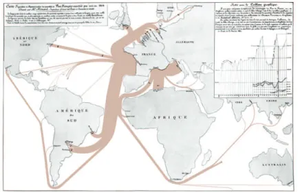
drawing or a set of trails, by spatially grouping graph edges or trails (which we next globally call paths). This way, the structure of the visualization becomes simpler and thereby easier to comprehend in terms of assessing relations that are encoded by such paths, such as finding groups of strongly interrelated nodes in a graph drawing, finding connections between spatial regions on a map linked by a number of vehicle trails, or discerning the motion structure of a set of objects by analyzing their trajectories (as depicted in figure 1.2).

Figure 1.2 – Early techniques related to bundling: flow map of French wine exports (Minard, 1864).

Bundling techniques stems from the field of graph simplification such as edge con-centration by Newbery, 1989 and the extensions of Sankey graphs by Tufte, 1992. Since then graph drawing simplification has been a major focus of edge bundling techniques, a term introduced by Dickerson et al., 2003 for the reduction of clutter in the drawing of a graph via node placement. The method was next extended to handle a wide variety of layouts and datasets; such as hierarchical graphs drawn in a 2D layout by Holten, 2006 and later 3D layout by the work of Collins and Carpendale, 2007 and Giereth, Bosch, and Ertl, 2008; Holten and Van Wijk, 2009 and Dwyer, Marriott, and Wybrow, 2006 for general graphs; Cui et al., 2008, Ersoy et al., 2011 and Lambert, Bourqui, and Auber, 2010b for spatial trail sets in a 2D embedding and Lambert, Bourqui, and Auber, 2010b on curved surfaces; Hurter, Ersoy, and Telea, 2013 for sequence graphs and Nguyen, Eades, and Hong, 2012 and Hurter et al., 2014a for dynamic and eye tracks; the work of Selassie, Heller, and Heer, 2011, Moura, 2015 and Peysakhovich, Hurter, and Telea, 2015 for generalized directed graphs; Telea and Ersoy, 2010 and Peysakhovich, Hurter, and Telea, 2015 for attributed graphs; McDonnell and Mueller, 2008, Palmas et al., 2014 and Palmas and Weinkauf, 2016 for parallel coordinate plots visualization; Martins et al., 2014 and Rauber et al., 2017 for multidimensional projec-tions; and the work of Yu et al., 2012, Böttger et al., 2014 and Everts et al., 2015 for 3D vector and tensor fields.

(15)

1.2. Research Questions and Approach 3

Along this growing interest to apply bundling to many data types, a wide array of bundling techniques has been proposed by different authors. Holten, 2006 proposed a technique based on control structures and Gansner et al., 2011 and Telea and Ersoy, 2010 proposed techniques based on graph simplification techniques. Later Holten and Van Wijk, 2009, Dwyer, Marriott, and Wybrow, 2006, Nguyen, Eades, and Hong, 2012 and Everts et al., 2015 based their techniques upon force directed models. Methods proposed by Phan et al., 2005, Cui et al., 2008, Lambert, Bourqui, and Auber, 2010b and Ersoy et al., 2011 are based on computational geometry techniques and Hurter, Ersoy, and Telea, 2012, Böttger et al., 2014, Moura, 2015 and Zwan, Codreanu, and Telea, 2016 use image-based techniques.

Overall, bundling goals largely follow those of early methods for simplifying graphs drawing as detailed in Herman, Melançon, and Marshall, 2000’s survey on Graph

vi-sualization and navigation in information vivi-sualization. And since then, bundling has

become an established tool for the creation of simplified visualizations of edge and trail data-sets.

However over the last years, the rapid development of the field, coupled with the diversity of its application domains (e.g., graphs, vehicle trails, eye tracking data, vector and tensor fields, all of them attributed or not and time-dependent or not), data types handled and a plethora of different algorithmic approaches, make it hard for users to choose the suitable method for a given use-case, or for researchers to focus on important areas of improvement. Moreover, the ever growing size and multi-dimensionality of data-set coupled with the inherent motive of visualizations to be as interactive as possible (i.e. having a low computational speed to provide instant feedback to users), constantly challenges the capabilities of bundling algorithms.

1.2 Research Questions and Approach

In this dissertation, we address the general research question:

äHow can we bridge the gap between the technical complexity of bundling

methods and the end-point users?

Bridging this gap means improving the understanding of bundling methods for users. Here, users can be researchers, engineers or developers with a different goal for each of them. To answer this my effort involves three aspects: a taxonomy, a framework and a tasks & uses-cases analysis.

Taxonomy: First, we must understand how bundling techniques relate to each other. Following the steps of the visual analytics process introduced by Keim et al., 2008 and from a user point of view, we ask the following question:

(16)

Framework: Given their large number and diversity, comparing all bundling methods from a technical viewpoint is a difficult challenge. For developers, a technical framework could help to compare in detail specific steps of specific algorithms. For researchers, this could help outlying technical limitations and future improvement areas.

ä Can we unify bundling techniques into a generic bundling framework to describe

them?

Tasks & uses-cases analysis: To fully use and understand bundling, we must know which tasks can be supported and in which context. Task taxonomies exist for information visualization in general (Brehmer and Munzner, 2013) as well as for graphs (Lee et al., 2006).

ä What are the tasks and proven use-cases bundling can solve?

Finally, in the context of multidimensional big data analysis, visualization tech-niques must be able to cope with the ever growing size of data-set. This is valid as well for bundling, where we aim towards fast interactions and aggregation based on user driven criteria (e.g. attribute-driven bundling). Here, we can ask ourselves:

ä How can bundling cope with very large multidimensional data-sets?

Application to the Study of Alzheimer’s Disease

As part of the multidisciplinary project called MEMOIRE, this thesis will report a new usage of edge bundling technique in the field of neuro-psychology.

Currently, approximately 860, 000 people are affected by Alzheimer’s disease in France. This estimation will possibly reach 2.1 million in 2040. This is why the study of Alzheimer’s disease has been identified as a major societal challenge. In the 3C cohort study (Antoniak et al., 2003), 3777 elderly people followed performed a lexi-cal evocation task (i.e. a fluency test) by saying the maximum number of city names within one minute. Subjects were followed during a 12 year period and some developed Alzheimer’s Disease (AD).

During the fluency test, practitioners handwrote the cited cities on paper. This task is directly related to the concept of cognitive maps (Tolman, 1948). The analysis of the list of cited cities created during the fluency tasks provides a unique opportunity to study the spatial mental representation of geographical space of elderly people, with a cross-sectional study, and the modification during the onset of Alzheimer’s dementia, with a longitudinal study. To the best of our knowledge, no previous work has inves-tigated this dataset thanks to interactive visualization methods (Card, Mackinlay, and Shneiderman, 1999). In the following chapters, we present our work which fills this gap. Throughout this application to the study of AD, we will answer the following questions.

(17)

1.3. Thesis Outline 5

First, as fluency tests were written on paper, the first step of our work was to produce an electronic health database as clean as possible. To support this task of cleaning, we asked ourselves the following question:

ä How can we use visual analysis tools to support efficiently the digitization and

cleaning of handwritten electronic health record data?

From the build database, we focused our research towards the development of a novel observation tool to analyze both the aging process of elderly and the onset of AD. In the framework of this thesis on bundling, our question was;

ä How and to what extend is bundling an efficient tool to generate visualization as

an observational and exploratory mean for scientist?

1.3 Thesis Outline

As a reading guide, each chapters of this dissertation contains a section numbered 0 located just after the chapter’s preamble. Section 0 of each chapter is composed of a summary of the given chapter in my native language, French. Non-French speaker can directly jump to the first section of the chapter (numbered 1). Whereas French speakers have access to the outlines of each chapters in their native language. Overall, this dissertation is divided into three parts, seven chapters and finishes with a chapter on conclusions and future work.

Part I: Bundling in the Information Visualization Context

The first part gives an overview of the place of bundling in the context of visualization through two approaches.

Chapter 2: Clutter Reduction for Node-Link Diagrams introduces the major definitions and concepts that relate to bundling techniques. We start by introducing the types of data (and their existing layout) that bundling works on. Then, we detail the basis of existing clutter reduction techniques in order to better understand the scope of bundling in the clutter reduction landscape. Finally, we introduce the main notations and a formal definition of path bundling, which we next specialize for graph and trail bundling.

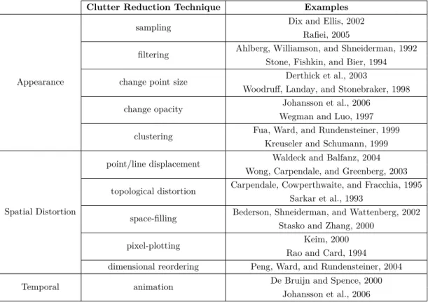
Chapter 3: A Data-based Taxonomy of Bundling Methods This chapter present our taxonomy of bundling methods according to the type of input data-set they work on (graphs vs trails, which we jointly refer to as paths). We show how this taxonomy is more clear-cut than the usual technique-based taxonomies that group bundling methods into data-driven, geometric, and image-based ones (see e.g. Zwan, Codreanu, and Telea, 2016; Zhou et al., 2013; Hurter, Ersoy, and Telea, 2012). More-over, our taxonomy helps users choose suitable algorithms for their data without having to dive into algorithmic details.

(18)

Part II: Unifying, Understanding and Improving Bundling Tech-niques

The second part of this dissertation works towards solving challenges of bundling tech-niques through three chapters. The first two chapters solve the challenges of comparing and choosing different bundling algorithms. Then we tackle the computational and scalability challenges of bundling techniques.

Chapter 4: Towards a Unified Bundling Framework In this chapter, we pro-pose a generic framework that describes the typical steps of all bundling methods in terms of high-level operations. We next show how such methods implement these steps. This helps one to compare in detail specific steps of specific algorithms, and complements the above-mentioned high-level taxonomy of bundling algorithms with technical insights. Our framework also helps outlining technical limitations of existing algorithms, suggesting future improvement areas.

Chapter 5: Bundling Tasks and Applications As outlined already, comparing bundling techniques is hard. We address this by proposing a description of tasks that bundling aims to address, following Lee et al., 2006’s and Brehmer and Munzner, 2013’s tasks taxonomies. We discuss how bundling can address these tasks, and also where salient limitations exist, in terms of the operations of our proposed framework. We also discuss ways (and challenges) to compare the results of different bundling methods. By this, we aim to provide a guide to the practitioner in selecting, customizing, testing, and possibly extending existing bundling methods to support optimally a given task set. Next, as bundling has gone far beyond simplified graph drawing we overview a wide set of bundling applications and relate these to the above-mentioned tasks. By this, we address limitations of papers which usually focus either on proposing a new technique or discussing a single application.

Chapter 6: Improving Bundling Scalability In this chapter, we bring bundling a step further towards its ability to cope with increasingly large data-sets. We present the FFTEB technique that addresses the joint edge-bundling challenges of computational speed and data volume, while keeping the quality of the results on par with state-of-the-art techniques. For this, we shift the bundling process from the image space to the spectral space, thereby increasing computational speed. We address scalability by proposing a data streaming process that allows bundling of extremely large data-sets with limited GPU memory.

Part III: Application to the Study of Alzheimer’s Disease

This part reports the use of path bundling techniques in the context of the study of Alzheimer’s Disease. Using the results of a French cohort study (3C Antoniak et al., 2003), we study both the effect of aging and the evolution of Alzheimer’s disease on the human brain through the study of fluency tests (Isaacs and Akhtar, 1972; Isaacs

(19)

1.3. Thesis Outline 7

and Kennie, 1973). The two following chapters expose the results of our work towards a better understanding of Alzheimer’s disease.

Chapter 7: A Visual Analytics Approach for Digitizing and Cleaning Health Data Prior to the analysis of bundled cognitive maps, this chapter presents visual analytics tools for electronic health records (EHR). Because the fluency tests were handwritten very quickly by a medical practitioner, some cities are abbreviated or poorly written. In order to analyze such data, we need to digitize and clean the data-set. As these tasks are intricate and error prone, we propose a novel set of tools, involving interactive visualization techniques, to help users in the digitization and data-cleaning process.

Chapter 8: Bundling Cognitive Maps In this chapter we illustrate our explo-ration and analysis process of our cleaned data-set built in chapter 7. Centered around the clutter reduction capabilities of our bundling technique for node-link diagrams, we show how bundling can efficiently be used as a visualization and exploration tool for neuro-psychologists in our study of Alzheimer’s disease. Specifically, we show how bundling allowed us to formulate new hypothesis on Alzheimer’s disease.

(20)

1.4 Introduction (Français)

Cette thèse s’inscrit dans le domaine de la visualisation d’information (InfoVis –

Infor-mation Visualization). Le domaine de l’InfoVis a pour but d’optimiser la bande passante

d’informations du canal visuel entre utilisateurs et visualisation. En d’autres termes, ce domaine vise à optimiser l’utilisation du système perceptif visuel pour optimiser la transmission et la compréhension d’informations graphiques.

Cette thèse se concentre sur un problème inhérent à la représentation de données denses et multidimensionnelles : l’occultation graphique.

1.4.1 Contexte et Motivation

Dans le domaine de la visualisation d’informations, les grands jeux de données multi-dimensionnelles sont analysés à l’aide de méthodes de visualisations interactives. Ces processus qui convertissent les données brutes en informations graphiques peuvent être décrits à travers la boucle de rendu de l’infovis (ou pipeline de l’InfoVis, Card, Mackin-lay et Shneiderman, 1999, figure 1.3). Dans cette boucle de rendu, les données brutes sont d’abord transformées en données structurées (transformation de données), puis les données structurées sont converties en structures et propriétés visuelles (représentation visuelle). Ensuite, les structures visuelles sont compilées pour former une ou plusieurs images (transformation visuelle) pour finalement permettre la perception visuelle des données par l’humain. L’InfoVis implique l’utilisation d’approches algorithmiques pour convertir les données brutes en visualisations compilées (ou images).

Figure 1.3 – Boucle de rendu de la visualisation d’informations d’après Card, Mackinlay et Shneiderman, 1999.

Si l’efficacité de telles approches a déjà été prouvée par le passé (Card, Mackinlay et Shneiderman, 1999), elles ont aussi montré leurs limites quant au traitement et à la visualisation de grandes quantités d’informations (Fekete et Plaisant, 2002). Comme les affichages et les écrans sont des espaces de dimensions finies limités par le nombre de pixels, la représentation visuelle de grande quantités d’informations introduit des représentations visuelles de plus en plus denses qui provoquent des problèmes d’oc-cultation des données. Dans l’optique de réduire les problèmes d’ocd’oc-cultation, plusieurs pistes de recherches et techniques de visualisation ont été développées (Ellis et Dix, 2007) et parmi elles, le bundling.

Le terme bundling fait référence à l’ensemble des techniques de simplification vi-suelle appliquées aux dessins de graphes ou aux jeux de trajectoires et qui consistent à spatialement grouper les liens d’un graphe ou les trajectoires ensembles. Dans la suite

(21)

1.4. Introduction (Français) 9

de cette thèse, nous désignerons par le terme générique chemins les liens d’un graphe ou les trajectoires d’un jeu de données. Ainsi, le processus de bundling ou d’agréga-tion visuelle de chemins permet de simplifier la structure de la visualisad’agréga-tion afin de la simplifier et donc de la rendre plus facile à comprendre en termes d’évaluation des rela-tions encodées par ces chemins comme par exemple : la recherche de groupes fortement interconnectés dans un graphe, la recherche de régions fortement interconnectées dans une carte de trajectoires ou encore pour discerner la structure des déplacements d’un ensemble d’objets à travers l’analyse de leurs trajectoires (comme détaillé en figure 1.4).

Figure 1.4 – Première apparition d’une technique ayant attrait au bundling : la carte des flux d’exportation des vins français

(Minard, 1864).

Les techniques de bundling prennent racine dans le domaine de la simplification de graphe à travers des techniques telles que la concentration de liens (edge concentration – Newbery, 1989) et les extensions aux graphes de Sankey par Tufte, 1992. Depuis, la simplification du dessin d’un graphe été l’objectif principal des techniques d’agrégation de lien dit de edge bundling, terme introduit par Dickerson et al., 2003 pour sa méthode consistant à réduire l’occultation dans le dessin de graphe via le placement de nœuds. La méthode a été ensuite étendue pour gérer un large éventail de techniques d’agencement de graphes et de types de jeux de données tels que : les graphes hiérarchiques dessinés en 2D par Holten, 2006 et plus tard en 3D grâce aux travaux de Collins et Carpendale, 2007 et Giereth, Bosch et Ertl, 2008 ; Holten et Van Wijk, 2009 et Dwyer, Marriott et Wybrow, 2006 pour les graphes génériques ; Cui et al., 2008, Ersoy et al., 2011 et Lambert, Bourqui et Auber, 2010b pour les trajectoires spatialisées en 2D et Lambert, Bourqui et Auber, 2010b sur des surfaces courbées ; Hurter, Ersoy et Telea, 2013 pour les graphes séquentiels et Nguyen, Eades et Hong, 2012 et Hurter et al., 2014a pour les graphes dynamiques et les tracés oculaires ; les travaux de Selassie, Heller et Heer, 2011, Moura, 2015 et Peysakhovich, Hurter et Telea, 2015 pour appliquer le bundling aux graphes attribués ; McDonnell et Mueller, 2008, Palmas et al., 2014 et Palmas et Weinkauf, 2016 l’ont appliquée aux visualisations de coordonnées parallèles ; Martins et al., 2014 et Rauber et al., 2017 pour les projections multidimensionnelles ; et les travaux de Yu et al., 2012, Böttger et al., 2014 et Everts et al., 2015 pour les champs de vecteurs 3D ou de tenseurs.

(22)

A travers l’intérêt croissant de l’extension des cas d’application du bundling à plu-sieurs types de jeux de données, un large éventail de techniques et d’algorithmes de bundling a été proposé par différents auteurs. Holten, 2006 a proposé une technique qui se fonde sur des structures de contrôles et Gansner et al., 2011 ainsi que Telea et Ersoy, 2010 ont proposé des techniques basées sur des techniques de simplification de graphes. Plus tard, Holten et Van Wijk, 2009, Dwyer, Marriott et Wybrow, 2006, Nguyen, Eades et Hong, 2012 et Everts et al., 2015 ont fondés leurs techniques sur des modèles de type interactions de forces. En parallèle, les méthodes proposées par Phan et al., 2005, Cui et al., 2008, Lambert, Bourqui et Auber, 2010b et Ersoy et al., 2011 se fondent sur le calcul de l’agrégation des liens grâce à des approches géométriques. Enfin, Hurter, Ersoy et Telea, 2012, Böttger et al., 2014, Moura, 2015 et Zwan, Codreanu et Telea, 2016 ont proposé des techniques basées image.

Globalement, le bundling suit largement les buts relatifs aux premières méthodes de simplification de graphes comme explicité par l’étude de Herman, Melançon et Marshall, 2000 sur la visualisation de graphes et la navigation dans le domaine de la visualisation d’information (graph visualization and navigation in information visualization). Et de-puis ce, le bundling est devenu un outil de référence pour générer des visualisations simplifiées d’ensembles de liens ou de trajectoires (i.e. d’ensembles de chemins).

Cependant au cours des dernières années, le développement rapide de ce champ de recherche couplé à la grande diversité des domaines d’application (e.g. graphes, trajectoires de véhicules, tracés oculaires, champs de vecteurs et tenseurs, tous ces jeux de données pouvant être attribués ou non et temporel ou non), du type de jeux de données traités et la pléthore d’approches algorithmiques, compliquent la tâche des utilisateurs pour choisir la méthode de bundling adaptée à leurs besoins, ou encore compliquent la tâche des chercheurs pour se concentrer sur les axes d’amélioration importants. De plus, l’augmentation constante de la taille et de la multi-dimensionnalité des jeux de données à traiter en parallèle avec le désir constant d’avoir des visualisations aussi interactives que possible (i.e. ayant une faible complexité algorithmique afin de fournir un retour rapide aux utilisateurs), challengent constamment les capacités des algorithmes de bundling.

1.4.2 Questions de Recherche et Approche

Au cours de cette dissertation, nous abordons la question de recherche suivante : äComment peut-on combler les lacunes entre la complexité technique

des algorithmes de bundling et les utilisateurs finaux ?

Combler ces lacunes reviens à améliorer la compréhension des méthodes de bund-ling par les utilisateurs. Dans notre cas, les utilisateurs sont soit des chercheurs, des ingénieurs ou des développeurs ayant chacun des objectifs différents. Pour y répondre, mon travail implique trois aspects : une taxonomie, un framework ainsi qu’une analyse des tâches et cas d’applications.

(23)

Taxonomie : En premier lieu, nous devons comprendre les relations entre les diffé-rentes techniques de bundling. En suivant la démarche des techniques d’analyse visuelle introduite par Keim, 2000 et en abordant un point de vue centré utilisateurs, nous nous posons la question suivante :

ä Comment s’organisent et se classifient les techniques de bundling en fonction du

type de jeu de données utilisé ?

Framework : Compte tenu de grand nombre et de la grande diversité des techniques de bundling, il est difficile de comparer ces dernières d’un point de vue technique. Pour les développeurs, un cadre d’application (ou framework) permettrait d’aider à comparer en détail des étapes spécifiques d’algorithme de bundling donnés. Pour les chercheurs, un tel framework permettrait de mettre en évidence les limitations techniques et les axes d’amélioration des techniques de bundling.

ä Peut-on unifier et décrire les techniques de bundling à l’aide d’une chaine de

traitement (ou pipeline) générique ?

Analyse des tâches et cas d’utilisation : Pour pouvoir utiliser les techniques de bundling à leurs plein potentiel, il est nécessaire de connaître les tâches spécifiques supportées par le bundling et leur contexte associé. Pour répondre à cette question, nous nous appuierons sur les taxonomies de tâches liées à la visualisation d’informations (Brehmer et Munzner, 2013) et liées aux dessins de graphes (Lee et al., 2006).

ä Quels sont les tâches ainsi que les cas d’utilisation avérés auxquels le bundling

répond ?

Enfin, dans le contexte de l’analyse de grandes quantités de données multidimension-nelles, les techniques de visualisation doivent pouvoir passer à l’échelle et être capable de traiter ces données. Cette assertion s’applique aussi au bundling qui vise à apporter une agrégation rapide des données en fonction de critères spécifiques à l’utilisateur (e.g. l’agrégation basée attributs) tout en conservant des interactions toutes aussi rapides. Ici, nous nous posons la question :

ä Comment le bundling peut-il faire traiter rapidement de grandes quantités de

don-nées multidimensionnelles ?

Application à l’Étude de la Maladie d’Alzheimer

S’insérant dans le projet multidisciplinaire MÉMOIRE, cette thèse rapporte un nouveau cas d’application du bundling au domaine de la neuropsychologie.

Actuellement, environ 860000 personnes sont touchées par la maladie d’Alzheimer en France. Ce chiffre devrait atteindre près de 2, 1 millions d’ici 2040. Ainsi, l’étude de la maladie d’Alzheimer a été identifiée comme un défi sociétal majeur. Dans le cadre de la cohorte 3C (Antoniak et al., 2003), 3777 personnes âgées ont dût réaliser une tâche

(24)

d’évocation lexicale (i.e. une tâche de fluence verbale) au cours de laquelle ils devaient citer le plus de villes possible en une minute. Ces sujets ont été suivis sur une période de 12 années et certains d’entre eux ont développé la maladie d’Alzheimer (Alzheimer’s

Disease – AD).

Au cours des tâches de fluences verbales, des médecins ont rapporté les villes ci-tées sur papier, ce qui nous donne l’opportunité d’étudier les villes cici-tées. Les études de Tolman, 1948 nous montrent que cette tâche est directement reliée au concept de cartes cognitives. C’est pourquoi l’analyse de la liste des villes citées pendant les tests de fluence verbales est une opportunité unique d’étudier la représentation mentale de l’espace géographique (cartes cognitives) chez les personnes âgées, grâce à une étude transversale, ainsi que d’étudier le développement de la maladie d’Alzheimer, grâce à une étude longitudinale. À notre connaissance, aucuns autres travaux n’ont entrepris l’étude de ce jeu de données à l’aide de techniques de visualisation interactives (Card, Mackinlay et Shneiderman, 1999). Les chapitres suivants présentent mes travaux à ce sujet. À travers cette application du bundling à la maladie d’Alzheimer, cette thèse répondra ainsi aux question suivantes.

Premièrement, comme les tests de fluence verbales ont été rapportés sur papier, nous avons dû créer une base de données informatisée (Electronic Health Record – EHR) contenant le moins d’erreurs possibles. Pour répondre à cette tâche complexe, nous avons répondu à la question suivante :

ä Comment peut-on efficacement aider la numérisation et le nettoyage de données

de santé à l’aide d’outils d’analyses visuelles ?

À partir de notre base de données construite et nettoyée, nous avons concentré notre recherche sur le développement d’un nouvel outil d’observation permettant à la fois l’analyse de l’impact processus de vieillissement mais aussi de l’impact du développe-ment de la maladie d’Alzheimer sur les tâches de fluences verbales. Dans le cadre de cette thèse consacré aux techniques d’agrégation visuelle, nous avons répondus à la question :

ä Comment et dans quelle mesure le bundling est-il un outil de visualisation de

données efficace pour générer des visualisations qui permettent aux scientifiques d’explorer et de faire de nouvelles observations de leurs données ?

1.4.3 Plan de Lecture

L’ensemble de ce manuscrit est rédigé en langue anglaise. Cependant, les points impor-tants de chaque chapitre sont résumés en français. Ces résumés se situent juste après le préambule de chaque chapitre et sont numérotés en section 0 dudit chapitre (e.g. la sec-tion 2.0 est la secsec-tion dédiée au résumé en français du chapitre 2). Dans son ensemble, le manuscrit est divisé en trois parties, sept chapitres et se termine par un chapitre de conclusion et de pistes de recherches entièrement traduit en français.

(25)

Partie I : Le Bundling dans le Contexte de la Visualisation d’Infor-mations

La première partie nous donne un aperçu de la place du bundling dans le contexte de la visualisation d’information à travers deux approches.

Chapitre 2 : Réduire l’Occultation des Diagrammes Nœuds-Liens Ce cha-pitre introduit les concepts et les définitions majeures qui ont trait aux techniques de bundling. Nous commençons par introduire les types de jeux de données (et leurs méthodes de dessins associées) que le bundling peut traiter. Puis, nous détaillons les bases des techniques de réduction d’occultation afin de mieux comprendre la place du bundling dans ce paysage. Enfin, nous introduisons les principales notations et notre définition formelle de l’agrégation de chemins, que nous explicitons ensuite aux cas de l’agrégation de graphes ou de trajectoires.

Chapitre 3 : Taxonomie des Méthodes de Bundling Dans ce chapitre, nous proposons une taxonomie des méthodes de bundling fondée sur la structure des don-nées d’entrée (i.e. graphes ou trajectoires). Bien qu’il existe d’autres taxonomies des méthodes de bundling purement fondées sur les différences techniques entre ces der-nières, comme illustré par Zhou et al., 2013, nous démontrons qu’une taxonomie fondée sur les structures d’entrée est plus claire et précise. De plus, cette approche “structure d’entrée” permet d’aider les utilisateurs à comprendre les techniques de bundling sans pour autant devoir aborder les spécificités de chaque méthode.

Partie II : Unifier, Comprendre et Améliorer les Techniques de Bundling

La seconde partie de ce manuscrit s’inscrit dans un travail de recherche visant à résoudre les défis des techniques de bundling à travers trois chapitres. Les deux premiers chapitres résolvent les défis liés à la comparaison et au choix des différents algorithmes de bundling existants. Puis nous nous attaquons aux défis de la complexité algorithmique et du passage à l’échelle des techniques de bundling.

Chapitre 4 : Un Pipeline Graphique Unifié des Méthodes de Bundling

Dans ce chapitre, nous proposons un cadre d’application générique permettant de dé-crire les étapes nécessaires pour le calcul de l’agrégation visuelle en terme d’opération haut niveau. Puis nous montrons comment les techniques existantes implémentent les différentes étapes de notre pipeline. Ce travail permet de comparer en détail les étapes spécifiques à certains algorithmes de bundling tout en complémentant notre taxonomie haut niveau en apportant des détails techniques. Ce pipeline permet aussi de mettre en évidence les limitations techniques des algorithmes existants pour suggérer des pistes d’améliorations futures.

(26)

Chapitre 5 : Tâches et Applications du Bundling Comme détaillé dans les précédents chapitres, il est difficile de comparer l’ensemble des techniques de bund-ling sans un cadre de référence commun et accepté. Dans ce chapitre, nous analysons comment les techniques de bundling s’intègrent dans la taxonomie de réduction d’oc-cultation de Ellis et Dix, 2007. Puis, nous proposons une description des tâches de visualisation (définies par Lee et al., 2006 et Brehmer et Munzner, 2013) auxquelles le bundling peut répondre. Ensuite, nous montrons comment le bundling peut répondre aux tâches identifiées et montrons les limitations des techniques actuelles. Pour ce faire, nous analysons un large spectre des cas d’utilisations du bundling et les mettons en lumière au regards des tâches de visualisation à résoudre. Ainsi, cette approche nous permet de mettre en lumière les limitations ainsi que les potentiels axes d’amélioration du bundling au regard des besoins utilisateurs.

Chapitre 6 : Une Nouvelle Technique de Bundling : FFTEB Dans ce chapitre, nous améliorons les capacités du bundling à traiter les grandes quantités de données. Nous présentons un nouvelle technique, FFTEB, qui résout les problèmes de passage à l’échelle des algorithmes de bundling. Afin de résoudre ces problèmes de vitesse de calcul et de complexité, nous changeons le paradigme de calcul du bundling en utilisant les propriétés de la transformée de Fourier (FFT). Puis nous résolvons les problèmes liés à la taille des jeux de données en proposant une méthode de transfert de données (data streaming) permettant l’agrégation de très larges jeux tout en s’abstrayant de la limite de taille de la mémoire des processeurs graphique.

Partie III : Application à l’Étude de la Maladie d’Alzheimer

Dans cette partie, nous rapportons l’utilisation du bundling dans le contexte de l’étude de la maladie d’Alzheimer. En utilisant les résultats de la cohorte française 3C (Anto-niak et al., 2003), nous étudions à la fois les effets du vieillissement et l’évolution de la maladie d’Alzheimer sur le cerveau humain à travers l’étude des tests de fluence verbale (Isaacs et Akhtar, 1972 ; Isaacs et Kennie, 1973). Les deux chapitres suivants exposent les résultats de notre travail visant à améliorer notre compréhension de cette maladie.

Chapitre 7 : Une Méthode d’Analyse Visuelle pour la Numérisation de Données de Santé Avant l’analyse des cartes cognitive agrégées, ce chapitre présente nos outils d’analyse visuelle pour la numérisation des données de santé (EHR). À cause du fait que les tests de fluence verbales ont été rédigés sur papier de façon rapide par un médecin, beaucoup de villes ont été abréviées ou mal écrites. Ainsi, pour pouvoir analyser ces données, nous avons dû numériser et nettoyer notre jeu de données. Comme ces tâches sont complexes et sujettes à des erreurs, nous proposons de nouveaux outils impliquant des méthodes de visualisation interactives, afin d’aider les utilisateurs dans le processus de numérisation et de nettoyage des données.

(27)

Chapitre 8 : Application du Bundling aux Cartes Cognitives Au cours de ce dernier chapitre, nous illustrons notre processus d’exploration et d’analyse de notre base de donnée des tests de fluence verbale (construite en chapitre 7). À l’aide de notre technique de bundling (exposée en chapitre 6), nous montrons que le bundling est un outil de visualisation et d’exploration efficace dans le cadre de notre étude sur la maladie d’Alzheimer. Plus spécifiquement, nous montrons que l’utilisation du bundling nous a permis de formuler de nouvelles hypothèses sur l’évolution de la maladie d’Alzheimer.

(28)

(29)

17

Part I

Bundling in the Information

Visualization Context

(30)

(31)

19

Chapter 2 Clutter Reduction for Node-Link

Diagrams

Bundling combines two concepts of Information Visualization: path drawing and clutter reduction. This chapter clarifies the main definition and concept for graph drawing and trails as well as clutter reduction techniques and criteria. We start by introducing the types of data (graph or trails) and their existing visualizations that bundling works on. Then we detail the basis of clutter reduction techniques to better understand the scope of bundling in this particular landscape. Finally, we introduce the main definitions and notations we deem necessary to understand the design space of bundling techniques.

(32)

20 Chapter 2. Clutter Reduction for Node-Link Diagrams

2.0 Résumé (Français)

Réduire l’Occultation des Diagrammes Nœuds-Liens

Les techniques de bundling (simplification de liens par agrégation visuelle) combinent deux concepts majeurs de la visualisation d’informations : le dessin de liens et la ré-duction d’occultation. Dans ce chapitre, nous clarifions les principales définitions et concepts relatifs aux dessins de liens (dessins de graphes ou dessins de trajectoires) ainsi que les techniques et critères relatifs à la réduction d’occultation de la visuali-sation de données. Nous débutons par l’analyse du type de données utilisables par les techniques de bundling (graphes ou trajectoires) ainsi que les moyens existants pour les visualiser (voir section 2.1). Ensuite nous détaillons les fondations des techniques de réduction d’occultation afin de mesurer la place du bundling parmi ces dernières (sec-tion 2.2). Enfin, nous introduisons les principales défini(sec-tions et nota(sec-tions nécessaires à la compréhension de l’espace de conception des algorithmes de bundling (section 2.3). Dans ce cours résumé en français, nous nous limiterons à définir les concepts et nota-tions relatifs aux techniques d’agrégation visuelle.

Definition de l’Opérateur Bundling

L’espace de conception des techniques de bundling est vaste et complexe contenant pléthore d’implémentations variées et de types de jeux de données utilisables. Dans l’optique d’unifier et d’améliorer la compréhension de cet espace, nous débutons notre travail par la définition des concepts et notations sur lequels se fondent cette thèse.

Les Objectifs du Bundling

Les graphes de grande taille, fortement connectés, issus d’applications concrètes ont beaucoup plus de liens que de nœuds. Au cause de cela, les représentations de ces graphes par des diagrammes nœuds-liens classiques deviennent rapidement inefficaces pour les explorer et les analyser. Ce problème est souvent référencé dans la littérature comme l’encombrement de liens (edge congestion, Carpendale et Rong, 2001, l’occul-tation de liens (visual clutter, Ellis et Dix, 2007) ou le problème de la boule de poils (hairball problem, Schulz et Hurter, 2013). Ainsi pour résoudre ce problème, plusieurs techniques existent (voir section 2.2 et Ellis et Dix, 2007) et parmi elles le bundling.

De manière informelle, le bundling échange l’occultation pour du ”sur-dessin“ (Te-lea et Ersoy, 2010). Cependant, bien qu’il y ait des dizaines d’articles sur le bundling, aucun ne définit formellement ce qu’est le bundling. Dans notre travail, nous argu-mentons qu’une telle définition est nécessaire si l’on souhaite comprendre le processus, comparer les méthodes et débattre des garanties et des limitations du bundling et plus généralement faire avancer la recherche sur le bundling.

(33)

2.0. Résumé (Français) – Réduire l’Occultation des Diagrammes Nœuds-Liens 21

Définition du Bundling

Soit G = (V, E ⊂ V × V ) un graphe avec des nœuds V = {vi} et des liens E = {ei}. Soit

d la dimension de l’espace de dessin dans lequel nous souhaitons appliquer le bundling

(généralement cette dimension est 2 ou 3). En parallèle, soit T = {ti} ce que nous appellerons un jeu de trajectoires comme définis par Phan et al., 2005 et Zhou et al., 2013. Une trajectoire t_i_{⊂ R}d est une courbe orientée. Généralement, les trajectoires décrivent les déplacements d’objets dans l’espace, e.g. des avions (Hurter, Tissoires et Conversy, 2009), des tracés oculaires (Peysakhovich, Hurter et Telea, 2015), des bateaux (Scheepens et al., 2011a), ou des personnes (Nagel, Pietsch et Dörk, 2016). Cependant, elles peuvent aussi représenter des courbes non liées à des déplacements, e.g. des lignes brisées dans la visualisation de type coordonnées parallèles (Parallel Coordinates Plots – PCP) (Inselberg, 2009) ou des tracés de tenseurs de diffusion d’IRM (Everts et al., 2015). Il est important de noter qu’en théorie des graphes la notion de trajectoire a une signification différente (un type de chemin dans un graphe pour lequel tous les liens sont distincts, voir Harris, Hirst et Mossinghoff, 2008). Soient G et T l’espace de tous les graphes et respectivement tous les jeux de trajectoires.

L’élément clé unifiant les graphes et les jeux de trajectoires est ce que l’on nomme l’opérateur de dessin D. Pour les graphes, D : G → Rd est typiquement une technique d’agencement ou de dessin des liens d’un graphe (voir Battista et al., 1998). Par analo-gie, nous noterons D(ei) et D(vi) comme la transformée (le dessin) des nœuds ei⊂ E, respectivement des liens v_i⊂ V . Pour les trajectoires, l’opérateur de dessin est la fonc-tion identité, i.e. D(ti) = ti, car les trajectoires sont déjà intégrées dans un espace géométrique. Nous unifions les deux espaces G et T en définissant P l’espace des jeux de chemins. Ainsi P dénote soit un graphe G soit un jeu de trajectoires T et par ana-logie, un chemin p ∈ P est soit un lien de graphe e ou une trajectoire t. Les chemins peuvent avoir des attributs additionnels, tels que la direction, le poids, la temporalité, un nom ou un type générique comme introduit par Peysakhovich, Hurter et Telea, 2015 et Diehl et Telea, 2014. Ainsi, un chemin p peut être vu comme un vecteur de dimension

n + d, avec n le nombre d’attributs et d la dimension spatiale du chemin.

Soit D ⊂ Rdl’espace de l’ensemble des dessins de chemins D(P ). Soit B : D → D un opérateur denotant l’agrégation (le bundling) d’un jeu de chemins ; et finalement soit

B(D(p)) la courbe représentant l’agrégation du chemin p. Alors B est une méthode de

bundling (ou d’agrégation) si :

∀(pi, pj) ∈ P × P |pi6= pj∧ κ(pi, pj) < κmax→

δ(B(D(pi)), B(D(pj))) δ(D(pi), D(pj)). Équation du bundling

Dans cette équation, δ est une distance entre les chemins de Rd, e.g. la distance de Hausdorff comme défini par Berg et al., 2010. κ : P × P → R+ _{est ce que nous} appellerons une fonction de compatibilité dénotant la similarité entre les chemins. En d’autres termes, quand κ tend vers 0 alors les chemins sont similaires, lorsque κ tend vers l’infini alors les chemins sont différents (i.e. incompatibles). Dans tous les cas, κ se doit d’être une fonction qui reflète la compatibilité géométrique des chemins dans leur espace

(34)

de dessins D(P ), i.e. lorsque κ(pi, pj) tend vers 0 alors δ(D(pi), D(pj)) tend lui aussi vers 0. De plus, κ peut inclure des compatibilités sur les n attributs additionnels (basés sur les données) mentionnés plus tôt, i.e. κ peut être modélisée par une distance entre chemins en dimension n + d (l’espace géométrique et des attributs, c.f. Peysakhovich, Hurter et Telea, 2015). Dans notre équation, seuls les chemins dont la compatibilité est inférieure à un seuil prédéfinis (κmax) doivent être bundlés – sinon le bundling de D(P ) subirait des déformations trop importantes pour être correctement analysé. De façon informelle, notre Équation du bundling définie que pour deux chemins compatibles alors le dessin bundlé de ces chemins B(D(p_i)) est géométriquement plus proche que le dessin original de ces premiers D(pi).

Différences et Similitudes entre Graphes et Trajectoires

Dans la litérature des techniques de bundling, les auteurs font souvent référence aux termes edge bundling ou graph bundling de manière non discriminée, même dans le cas où les données à bundler sont des trajectoires. Ainsi, il est donc important de clarifier les différences et ressemblances entre le bundling de ces deux entités.

Pour résumer, les graphes et les trajectoires sont deux types de données radicalement différents – le premier n’étant pas lié à un espace géométrique (pour ce faire nous avons besoins du dessin du graphe) ; le second étant par définition intégré dans un espace géométrique (Euclidien). Les trajectoires sont typiquement des courbes orientées, alors que les liens d’un graphe ne le sont pas forcément. En théorie, la plupart des algorithmes de bundling peuvent bundler des dessins de graphes ou des trajectoires. Cependant, choisir le correct algorithme de bundling pour agréger un jeu de chemins donné est guidé par des critères plus subtiles que simplement le type de données d’entrée (e.g. la définition des fonctions de compatibilités, la quantité d’agrégation à fournir ou le type de structure à mettre en valeur). Tous ces aspects sont importants pour comprendre et utiliser de façon optimale le bundling, comme nous allons le démontrer dans la suite de cette thèse.

Au cours de ce chapitre, nous avons établi le cadre global de visualisation dans lequel les techniques de bundling prennent racine. Nous avons introduit les différents principes et méthodes de mise en forme des différents jeux de données utilisables par le bund-ling : les graphes et leurs techniques de dessins (voir section 2.1) et les trajectoires. En section 5.1.1, nous avons détaillé et explicité les techniques de réduction d’occultation existantes qui nous permettrons dans les chapitres suivant d’améliorer la compréhension et la place du bundling dans l’ensemble des techniques de réduction d’occultation. En-fin, nous avons défini (et résumé en français) les principes importants et les principales définitions propres au bundling (e.g. Équation du bundling) nécessaire pour débuter notre analyse de l’espace des techniques de bundling dans les chapitres suivants. Au cours des chapitres à venir, nous exposerons le bundling sous 3 angles différents, en partant d’une taxonomie orientée type de jeu de données d’entrée (chapitre 3) vers la construction d’un pipeline unifié des méthodes de bundling (chapitre 4) et une analyse des tâches et des domaines d’application du bundling (chapitre 5).

(35)

2.1. From Data to Point/Line Visualization 23

2.1 From Data to Point/Line Visualization

Bundling aims at providing a visual simplification by spatial grouping similar lines. This process requires the ability to represent information embedded in a given data-set to be represented as a point/line visualization. In this section, we will detail two formalisms of data-sets structure and how each type of data-set can be plotted on a screen in order to be bundled.

2.1.1 Graphs

“Graphs in general form one of the most important data models in computer science”, Beck et al., 2014. Formally, any relational structures consisting of a set of entities and relationships between those entities can be modeled as graphs. In the last two decades, graph theory and graph drawing have played a large part in the research themes of Human-Computer Interaction and Information Visualization. In this subsection, we will define and present the basis of graph drawing, specifically, how we transform a graph based data-set into a visual structure. This subsection highlights existing surveys of the field (i.e. Von Landesberger et al., 2011, Herman, Melançon, and Marshall, 2000, Battista et al., 1998).

Definitions

What we call graph refers to a set of vertices and a set of edges that connect pairs of vertices. A graph is a pair of these sets, G = (V, E) where V is a set of vertices and E is a set of edges between vertices (i.e. E ⊂ V2 e.g. an edge e = (v₁, v2) where v1∈ V and v2∈ V ), see Diestel, 2000. This definition can be extended by attaching attributes to vertices and/or edges to denote their type, size, or some other application related information.

The formal model of graph is further refined and classified into undirected and

directed graphs (Herman, Melançon, and Marshall, 2000). A directed graph (or digraph)

is defined similarly with the exception that the elements of E, called directed edges, are ordered pairs of vertices. In other terms, in a directed graph, for two vertices v1, v2, (v1, v2) 6= (v2, v1). Conversely, for an undirected graph, ∀v1, v2, (v1, v2) = (v2, v1). A graph containing both directed and undirected edges is called a mixed graph.

In graph theory, a (directed) path in a (directed) graph G is a sequence (v1, v2, ..., vn) of distinct vertices where v_i∈ V and (v_i, vi+1) ∈ E. A (directed) path is a (directed)

cycle if (vh, v1) ∈ E. Similarly, a directed graph that has no directed cycles is called a directed acyclic graph (DAG).

A tree is a connected undirected graph without cycle (Diestel, 2000). A Tree T is called rooted when one vertex r is distinguished as a so called root node: T = (V, E, r). In graph drawing, we often called such rooted tree a hierarchical graph. However, in the formal framework of mathematical graph theory, a hierarchical graph is a DAG (meaning a node can have several paths to the root node).

(36)

Additionally, we call compound graph C as a pair (G, T ) where G = (V, EG) and

T = (V, ET, r) that share the same set of vertices, such that:

∀e = (v1, v2) ∈ EG, v1∈ path/ T(r, v2) & v2∈ path/ T(r, v1) (2.1) Relationships between vertices are expressed by the tree T . Here, vertices sharing a common parent in T belong to the same “branch” (or “group”) of T .

Graphs may also change over time, forming what we call dynamic graphs. Time dependent changes can affect the attributes of nodes and edges but also the graph structure. A dynamic graph G(t) = (V (t), E(t)), t ∈ R+. A a given time t_i, G(t_i) is called a frame. Two different forms of dynamic graphs are known: streaming graphs and sequence graphs.

In a streaming graph G = (V, E), each edge ei∈ E has a so-called lifetime [tstarti , tendi ], of duration λj= tendi − tstarti , where tstarti < tendi . That is, ei exists only between tstarti and tend_i . The dynamic graph G(t) thus contains all edges e_i∈ E that are alive at t,

i.e. for which tstart_i ≤ t ≤ tend

i . The same holds for the streaming graph’s nodes vi∈ V . Streaming graphs can be available in an online manner – that is, one does not know upfront all moments tstart_i and tend_i .

Sequence graphs are, as their name says, ordered sets G = {Gi} of static graphs

Gi= (Vi, Ei). In contrast to streaming graphs, edges Ei do not have a lifetime, but belong to a single frame i. They typically capture a system’s structure at several discrete time moments ti. Well-known examples are the set of call graphs mined from the several revisions of software system stored in a software repository (Diehl and Telea, 2014 and Reniers et al., 2014). In practice, the frames Gi are usually not unrelated, but have nodes and edges which capture the evolution in time of the same items. For instance, two edges ei_a∈ Ei_{and e}i+1

b ∈ Ei+1can represent the same call relation in two consecutive frames of a software system. Such links relating information between different sequence frames can be modelled by a so-called correspondence function c : Ei → Ei+1_{∪ {∅}.} Here, c(e ∈ Ei) yields an edge e0∈ Ei+1 _{which logically corresponds to e, if such an} edge exists in Ei+1, or the empty set, if there is no correspondence, i.e. if e disappears in the transition from Gi to Gi+1.

Overall, we can classify existing graphs as summarized in figure 2.1.

Figure 2.1 – Classification of graphs based on their time-dependence and graph structure.

(37)

Graph Layout for Node-link Diagrams

Here, it is important to emphasize that a graph and its drawing are quite different objects. Per definition, a graph does not have any drawing and is not embedded in any kind of Hilbertian space. “In general a graph has many different drawings” (Battista et al., 1998), and choosing the correct layout for a given graph is a recurrent research of the Graph Drawing and Information Visualization community. Overall, graph layout techniques aim at optimizing several criteria depicted in three groups in the recent survey “Visual Analysis of Large Graphs: State-of-the-Art and Future Research Challenges” by Von Landesberger et al., 2011 (see Von Landesberger et al., 2011 section 3). These three groups are:

• General criteria: They encompass criteria such as reduction of visual clutter or maximization of space efficiency.

• Dynamic graphs: Maximization of display stability between time points or reduc-tion of cognitive load.

• Aesthetic scalability criteria: These criteria refer to graph readability for larger graphs, i.e. scalability in number of vertices, edges, and graphs.

According to Von Landesberger et al., 2011, despite being important these criteria cannot be simultaneously optimized and are not sufficient to design a good layout which is usually data and/or task dependent. Therefore, multiple graph layout are fundamental to exploratory graph visualization.

A plethora of graph layout methods and algorithm exist in the literature and gener-ally a graph layout methods is optimized for a specific type of graph (tree, coumpound, directed graph...). An extensive study of existing graph layout methods is detailled by Von Landesberger et al., 2011 in section 3. We can note a few classes of layout techniques for static graphs studied by Von Landesberger et al., 2011:

• Space-Filling techniques: They typically try to use the full area of the display to present the hierarchy of a graph (see figure 2.2a). Here, the spatial position of nodes are employed to display edges between nodes by using either closeness or enclosure.

• Matrix-Representation: These techniques displays the adjacency matrix of a given graph. Here each row and column displays a node and the links and attribute are displayed by a cell (see figure 2.2b).

• Node-Link Techniques: They are by far the most used layout methods for graphs. Here, the idea is to represents nodes as points and links as edges (see figure 2.2c). Node-link layout are generally embedded in 2 or 3 dimensional spaces. Many techniques exist to optimize the aforementionned layout criteria. Von Landes-berger et al., 2011 distinguish force-based, constraint-based, multi-scale, layered, and non-standard layouts.

(38)

• Hybrid approaches: As their name suggests, such approaches mix two or more of the different aforementioned layout methods and/or classes. For example, it can mix node-link and matrix layout as depicted in figure 2.2d.

(a) Space-Filling (b) Matrix (c) Node-Link (d) Hybrid Figure 2.2 – Four classes of graph layout techniques. Von Landesberger

et al., 2011

Dynamic graphs generally use the static graphs layouts techniques in conjunction with other time-series visualization such as animation or juxtaposition. An extended survey of the layout and visualization techniques for dynamic graphs is provided by Beck et al., 2014 in “The State of the Art in Visualizing Dynamic Graphs”.

2.1.2 Trail-sets

Separately, we define a trail-set T = {t_i} according to Phan et al., 2005 and Zhou et al., 2013. A trail-set is a collection of trails that typically describe the motion of shapes or objects in space, e.g. airplanes (Hurter, Tissoires, and Conversy, 2009), eye tracks (Peysakhovich, Hurter, and Telea, 2015), ships (Scheepens et al., 2011a), or persons (Nagel, Pietsch, and Dörk, 2016). As such a trail ti ⊂ Rd is an oriented curve in a Euclidian space. However, trails can also be curves unrelated to motion, e.g. polylines in a parallel coordinate plot (PCP) (Inselberg, 2009) or DTI tracts (Everts et al., 2015). Conversely to graphs, trail-sets are in essence spatially embedded into an Euclidian space (generally 2 or 3 dimensional). Similarly to graphs, we distinguish different categories of trail-sets: undirected or directed trail-sets and time dependent ones (see figure 2.3). Note that, in graph theory, the term trail has a different meaning, i.e, a type of walk on a graph in which all edges are distinct (as defined by Harris, Hirst, and Mossinghoff, 2008).

Figure 2.3 – Classification of trails based on their time-dependence and dimensional embedding.

(39)

2.1.3 Graph vs Trail-sets Differences and Similarities

Bundling literature often refers to ‘edge bundling’ or ‘graph bundling’ indiscriminately, even when the actual data being bundled are trail-sets. It is thus important to clarify both differences and similarities between (the bundling of) graphs and trail-sets.

Differences

• A graph G does not have a given spatial embedding. Only a graph drawing does. So, one bundles graph drawings, not graphs. The distinction is crucial, as the drawing D(G) is an extra degree of freedom – the same G can have multiple drawings D(G). Of course, one can use graph information, e.g. edge attributes, to influence bundling – see the discussion of compatibility function in section 2.3.1. Yet, having a layout D(G) is mandatory; without it, we cannot bundle a graph as a non-spatial, abstract object.

• In contrast to graphs, a trail-set T is always spatially embedded, by definition. This embedding encodes relevant data, e.g., geo-positions of vehicle movements, or variable values in a PCP. Hence, bundling a T is far more delicate than bundling a D(G): Deforming the former can distort spatially-encoded information; deform-ing the latter only distorts decisions of the graph-drawdeform-ing algorithm, but none of the raw data G.

• Both graphs G and trail-sets T can be directed or not. However, most trail-sets are directed, as they represent motion trajectories.

• Nodes v_i in a graph G are typically shared by multiple edges e_i. After all, this defines a graph. In contrast, endpoints of trails ti do not have to match. Hence, a trail-set T is a less structured dataset than a graph G.

Similarities

• Bundling both graph drawings and trail-sets can be expressed by the same for-malism (as defined in section 2.3, Bundling equation). Of course, the meaning of the compatibility functions can be different for graphs vs trail-sets, but the same can hold for two use-cases featuring graphs or trail-sets.

• Given the above, the same algorithm B can be used to bundle graphs and trail-sets, if it delivers a visual simplification (and implicitly, path deformation) which is suitable for the problem at hand. This is well visible in many bundling papers which propose the same bundling method for both graphs and trail-sets.

• The overarching goal of bundling – reducing clutter in a path drawing so that its core structure stands out – is common to both graph drawing and trail-set bundling.