Research Article
Transmissivity Identification by Combination of CVFEM and
Genetic Algorithm: Application to the Coastal Aquifer
Hassan Smaoui
,
1,2Abdelkabir Maqsoud,
3and Sami Kaidi
1,21CEREMA/DTecEMF, 134, Rue de Beauvais, CS 60039, 60280 Margny-L`es-Compi`egne, France
2Sorbonne Universit´e, Universit´e de Technologie de Compi`egne, Laboratoire Roberval/LHN, FRE-CNRS 2012,
CS 60319, 60203 Compi`egne, France
3Universit´e du Qu´ebec en Abitibi-T´emiscamingue (UQAT) 675, 1`ereAvenue, Val-d’Or (QC) J9P 1Y3, Canada
Correspondence should be addressed to Hassan Smaoui; hassan.smaoui@cerema.fr Received 31 December 2018; Accepted 11 June 2019; Published 29 July 2019 Academic Editor: Saeed Eftekhar Azam
Copyright © 2019 Hassan Smaoui et al. This is an open access article distributed under the Creative Commons Attribution License, which permits unrestricted use, distribution, and reproduction in any medium, provided the original work is properly cited. The solution of inverse problems in groundwater flow has been massively invested by several researchers around the world. This type of problem has been formulated by a constrained optimization problem and this constraint is none other than the direct problem (DP) itself. Thus, solving algorithms are developed that simultaneously solve the direct problem (Darcy’s equation) and the associated optimization problem. Several papers have been published in the literature using optimization methods based on computation of the objective function gradients. This type of method suffers from the inability to provide a global optimum. Similarly, they also have the disadvantage of not being applicable to objective functions of discontinuous derivatives. This paper is proposed to avoid these disadvantages. Indeed, for the optimization phase, we use random search-based methods that do not use derivative computations, but based on a search step followed only by evaluation of the objective function as many times as necessary to the convergence towards the global optimum. Among the different algorithms of this type of methods, we adopted the genetic algorithm (GA). On the other hand, the numerical solution of the direct problem is accomplished by the CVFEM discretization method (Control Volume Finite Element Method) which ensures the mass conservation in a natural way by its mathematical formulation. The resulting computation code HySubF-CVFEM (Hydrodynamic of Subsurface Flow by Control Volume Finite Element Method) solves the Darcy equation in a heterogeneous porous medium. Thus, this paper describes the description of the integrated optimization algorithm called HySubF-CVFEM/GA that has been successfully implemented and validated successfully compared to a schematic flow case offering analytical solutions. The results of this comparison are qualified of excellent accuracy. To identify the transmissivity field of the realistic study area, the code HySubF-CVFEM/GA was applied to the coastal “Chaouia” groundwater located in Western of Morocco. This aquifer of high heterogeneity is essential for water resources for the Casablanca region. Results analysis of this study has shown that the developed code is capable of providing high accuracy transmissivity fields, thus representing the heterogeneity observed in situ. However, in comparison with gradient method optimization the HySubF-CVFEM/GA code converges too slowly to the optimal solution (large CPU-time consuming). Despite this disadvantage, and given the high accuracy of the obtained results, the HySubF-CVFEM/GA code can be recommended to solve in an efficient and effective manner the identification parameters problems in hydrogeology.
1. Introduction
The coastal aquifers play an important role in the socioe-conomic development of the coastal plains [1–4]. These costal aquifers are particularly exposed to over-exploitation problems that can induce aquifer salinization [5–7]. Also, as presented in the Intergovernmental Panel on climate change (IPCC, 2007), climate changes will provide variations in the
sea level, temperature and rate and intensity of precipitation. All these changes will affect freshwater resources, in terms of both quantity and quality [8].
The climate change impacts are mainly evaluated using numerical groundwater modeling for both flow and trans-port phenomenon (Moustadraf et al., 2008). The numer-ical groundwater modeling requires many hydrodynamic parameters such as the water budget, the storativity, the
Volume 2019, Article ID 3463607, 14 pages https://doi.org/10.1155/2019/3463607
piezometric level (also called the head), the transmissivity, and specific yield. These parameters are usually obtained from some in situ pumping field and/or laboratory tests. However, in situ measurements, which are usually performed in a limited number of points of the study area (due to their cost), may prove insufficient to deduct the transmissivity coefficient. Besides this major inconvenience we also note the difficulty of the logistic realization of the measurement itself (access to the measurement site). Consequently, mea-surements can be considered as not economically feasible especially in the case where the funds for scientific research are very limited.
Given these drawbacks, mathematical models have emerged as powerful tools to complete lack of information to estimate correctly the transmissivity coefficient. With the spectacular advances in information technology, the mathematical models combined with the optimization tools became essential for geosciences modeling including flows and associated transport in groundwater.
To ensure an optimal management of the groundwaters, we need a good estimation of the head obtained by solving the Darcy’s equation. The quality of this estimation depends strongly on the quality of the transmissivity values (main flow parameter). However, the accurate knowledge of this parameter is difficult to obtain because of the heterogeneity due to real geological formation of the aquifers and the nature of the flows, or both. Consequently, the mathematical models and their discretization methods must be chosen judiciously in order to best approximate the studied phenomena. For a known transmissivity field, several codes solving Darcy’s equation have been proposed to compute the hydraulic potential (see for example PMWIN-MODFLOW, FEFLOW, GMS, HySuf-FEM). This is called “the direct problem”. However, a good prediction of the head requires prior identification of parameters involved in the Darcy’s equation (this is “the inverse problem”).
For over four decades inverse problem for groundwater flow has been studied by different authors (here, we cite only more recent studies: Katsifarakis et al., 1999; [9–16]) and a good review of this strategy to solve the problem can be seen in Yeh, 1986 and Carerra, 1988 [17, 18]. The strategy to identify the parameters by inverse problem consists of a combination of a computer code for flow (hydrodynamic model) and an optimization computer code. The optimization procedure was approached by a large number of optimizers: determinis-tic ones as gradient-based methods, Newton methods, quasi-Newton with interior points methods or stochastic ones as evolution strategies (ESs), artificial neural network (ANN) or genetic algorithms (GAs). The flow can be performed by different approximation methods as finite difference method (FDM), finite element method (FEM), finite volume method (FVM), meshless method, and many others.
In this paper, the CVFEM was chosen to compute the hydraulic head. This choice was motivated by the ability of this method to conserve the physical quantities involved in the hydrodynamic model (as FVM) and also by its ability to handle complex boundaries of the study area (as FEM). For the optimization step, we adopted the genetic algorithm. Although this type of algorithm is slower compared to
other algorithms (gradient-based algorithms), GA has been selected in this paper for its capacity to converge to a global optimum without using derivatives of the objective, also because it is well suited in particular on convex, non-separable, ill-conditioned, multi-modal or noisy objective functions. In addition, note that the inverse problem in groundwater flow is characterized by the identification of the large-size parameters (number of mesh node of the direct problem). It is also characterized by an objective function having no analytical expression, but built from the simulation results from the hydrodynamic model. These characteristics make usually the inverse problem in groundwater flow impossible to resolve by conventional deterministic methods. This is another reason which motivated our choice on a stochastic method particularly the GA.
This paper is organized as follows: Section 2 outlines the mathematical formulation that describes the CVFEM method for the direct problem and the GA for optimization procedure. Section 3 is devoted to the presentation of numer-ical results (academic tests) on the validation of the direct problem and the coupling “direct problem/optimization” procedure. At the end of this section we present the applica-tion of the combinaapplica-tion “CVFEM/GA” to the realistic case of a coastal aquifer to determine the transmissivity field. Finally, discussion and conclusions are presented in the last section.
2. Mathematical Model
At the macroscopic scale, the rate at which the water flow in a soil is quantified using a variable that is referred to as the Darcy velocity or specific discharge →𝑞 . This variable, which has the dimensions of velocity, is defined as the discharge per unit cross area of soil that includes both the pore space and the grains in a flow section. It is also defined as a vector in the direction of flow, where its magnitude is equal to the volume of water flowing per unit time through a unit cross-sectional area normal to the direction of flow.
2.1. Governing Equations. Assume that the flow is stationary
or that both fluid and porous media are incompressible. By the mass conservation law, the continuity equation holds, i.e.,
∇.→𝑞 = 𝑓 (1)
where the function𝑓 represents sources or/and sinks terms. Inside the saturated zone if we assume that the specific discharge →𝑞 is derived from a potential 𝜑 via the hydraulic conductivity tensor 𝐾, we obtain the unsteady Darcy law given by
𝜕𝜑
𝜕𝑡 − ∇. (K∇𝜑) = 𝑆 (2) where𝑆 is the source (or sink) term.
An exact solution of a potential flow problem (2) can be derived only in special cases. Therefore, numerical methods are the major tool for solving such problems in practice. A
common approach is to rewrite this into the following partial differential equation (PDE) with its boundary conditions:
(𝐷𝑃) { { { { { { { { { { { { { { { { { 𝜕𝜑 𝜕𝑡 − ∇. (K∇𝜑) = 𝑆 𝑖𝑛 Ω 𝜑 = 𝜑𝐷 𝑖𝑛 𝜕Ω𝐷 →𝑛 .→𝑞 = 𝜑 𝑁 𝑖𝑛 𝜕Ω𝑁 𝜑 (𝑥, 0) = 𝜑0(𝑥) 𝑖𝑛 Ω (3)
where Ω is the domain area, 𝜕Ω𝐷 is the boundary of the imposed Dirichlet condition, 𝜕Ω𝑁 is the boundary of the imposed Neumann condition, and →𝑛 is the outward normal vector to the Neumann boundary𝜕Ω𝑁.The equation (3) is known by Darcy equation. The average velocity →V of the fluid can be deducted from →𝑞 by →V = →𝑞/𝑝, where 𝑝 is the porosity of the studied area. Otherwise, we note that, according to Ciarlet, [21], the problem (3) is a well-posed problem; i.e., the solution exists, is unique, and depends continuously on the data.
The vast majority of solvers of the Darcy equation use finite difference, finite volume, or finite element approxi-mation in space. Numerous numerical approaches can be enumerated for solving equation (3). All these approaches are based on a discrete partition of the spatial domain of interest. The partition can be a structured grid or more generally an unstructured mesh. The numerical scheme that approximates the solution then consists in proposing an approximation of this solution on the discretized domain. In other words, we constrain the approximate solution to verify the Darcy equation to achieve a linear system (or non-linear) whose approximate solution is the unknown of such a system. The Darcy equation has been massively solved by classical methods (MDF, MEF, MVF). It is difficult to conclude on the effectiveness of this or that method, but it all depends on what one wishes to privilege between mass conservation, accuracy or a minimum computation (CPU time) [22, 23]. Today, we are witnessing a great growth in the use of CFD to solve real problems (environmental, industrial, etc.). To take into account the irregular boundaries of this type of problem, it has become necessary to choose dis-cretization methods allowing flexibility in the management of boundary conditions on boundaries of complex geometries. Some numerical methods based on orthogonal or curvilinear coordinate structured meshes approaching boundaries are frequently used to calculate flows in irregular geometries, with satisfactory results. However, we also observe that methods based on unstructured finite element meshes have become the reference methods for the prediction of flows in complex geometries.
In this work and to solve the Darcy equation, we adopt the CVFEM method on a FEM type unstructured mesh. In CFD, this method combines the advantages of finite volume methods over regular mesh and finite element methods. Indeed, the CVFEM formulation in terms of flows only translates the physical principle of the local and global conservation of a quantity evolving in a volume of elementary control. But in particular, CVFEM allows efficient handling of pressure/velocity coupling. On the other hand, when
CVFEM is formulated on a finite element mesh, we inherit the geometric flexibility and the use of the basis functions of the Sobolev space to interpolate the solution on a control volume [24, 25].
2.2. The CVFEM Discretization. Before beginning the
math-ematical formulation of this method, a brief description of some spaces is necessary. Consider a limited open setΩ ⊂ R2 having an Lipschitzian and continue boundary𝜕Ω. We
define𝐿2(Ω) as being the space of real functions 𝑢 such 𝑢2 is measurable functions. square. We define𝐻1(Ω) also as the subset containing functions of𝐿2(Ω) whose first derivatives are also in𝐿2(Ω). Similarly, we define 𝐻1𝑔(Ω) the subset of 𝐻1(Ω) whose functions are equal to 𝑔 on the on the boundary
𝜕Ω of Ω. Finally, we define the inner product of the space of 𝐿2(Ω)
∀𝑢, V ∈ 𝐿2(Ω) (𝑢, V)𝐿2(Ω)= ∫
Ω𝑢 (𝑥) V (𝑥) 𝑑𝑥
(4)
The numerical solution of equation (3) begins with the arbitrary subdivision of the domain Ω into 𝑁𝑒 elements (for example triangular elements) denoted(𝑇𝑘)𝑘=1,...,𝑁𝑒 and 𝑁𝑛 nodes. The family of triangles 𝑇𝑘 forms what is called the triangulation Tℎ, indexed by the parameter ℎ which designates the length of the largest sides of all the triangles of the mesh. This triangulation admits𝑁𝑛nodes which are the vertices of the set of triangles covering the domain. In the rest of this document, we omit the subscript “𝑘” of the triangle𝑇𝑘, but for any triangle we will note𝑇 ∈ Tℎ. The triangulationTℎallows the approximation of the domainΩ byΩℎ= ⋃𝑇∈Tℎ𝑇. We can now give the piecewise linear finite element spaces by
𝐻ℎ= {V ∈ C0(Ωℎ) : ∀𝑇 ∈ Tℎ, V/𝑇 𝑖𝑠 𝑙𝑖𝑛𝑒𝑎𝑟} (5) whereC0(Ωℎ) is the set of continuous functions on Ωℎand V/𝑇 is the restriction of the function V on the triangle 𝑇. In the same manner, we define𝐻ℎ,𝑔(Ω) = 𝐻ℎ∩ 𝐻𝑔1(Ω).
The CVFEM method must be applied to the integral for-mulation of the Darcy equation. This forfor-mulation translates the physical principle of the conservation of the𝜑 transferred scalar quantity in the small control volumeV.
∫
V
𝜕𝜑
𝜕𝑡𝑑V − ∫V∇. (K∇𝜑) 𝑑V = ∫V𝑆𝑑V (6)
To preserve this important physical principle in the numerical results, CVFEM uses a weighting function equal to the unit on all the volume of control associated with the node of the computation and zero elsewhere. Consequently, the CVFEM discretization imposes naturally the physical principle of conservation in the control volume V. Thus, the CVFEM admits an easy physical interpretation and its numerical solution meets the requirements of conservation both locally and globally even in the case of use of a coarse mesh.
k(3) →n →n →n i(1) j(2) (a) f2 f1 fp 2 3 (b) (c) k(3) j(2) b g c a p11 p21 →n 12 →n 11 i(1) (d)
Figure 1: The construction of control volumes: (a) the cell-centered control volume; (b) the vertex-centered control volume, (c) the dual mesh and (d) the sub-control volume. Notation(𝑖(1), 𝑗(2), 𝑘(3)) means that for a triangle 𝑇, the global numbering is (𝑖, 𝑗, 𝑘) and the local numbering is(1, 2, 3).
CVFEM uses two volume control types: cell-centered volume control and vertex-centered volume control. The first type is to consider the triangular element as a control volume (Figure 1(a)), while the second type builds support around a node𝑖 to use the dual mesh (Figure 1(c)). Several methods have been used for the construction of the control volumeV𝑖 based on the support of nodes𝑖. As far as we are concerned, we use volumes of controls of the dual mesh built as follows: for a node𝑖 of the mesh, one searches all the triangles having common node𝑖. So the control volume V𝑖 will be formed by joining the centers of gravity of all the triangles around the node𝑖 (Figure 1(b)). It is considered that the boundary Γ𝑖 = 𝜕V𝑖of the control volumeV𝑖consists of𝑝𝑖elementary facets𝑓𝑚. We note the set of these facets byF𝑖 (card(F𝑖) =𝑝𝑖). It should be noted that if the control volume V𝑖 is constructed from𝑝𝑖triangles, thenV𝑖is the union of𝑝𝑖 sub-control volume(S𝑖,𝑚)𝑚=1,𝑝𝑖which is the quadrilateral (iagc) (See Figure 1(d)).
2.3. The Control Volume Formulation. After the step of the
studied area discretization in elementary control volume, the different numerical methods of approximations consist in approaching the solution on the mesh nodes based on the physical principle of conservation. Like the other methods CVFEM applies this principle on the control volumeV𝑖to
the equation (6). By using the Gauss divergence theorem, we have ∫ V𝑖 𝜕𝜑 𝜕𝑡𝑑V − ∫𝜕V𝑖 (K∇𝜑) →𝑛 𝑑𝑙 = ∫ V𝑖 𝑆𝑑V (7) where →𝑛 is the outward unit normal vector to 𝜕V𝑖. For a physical quantity𝜓, the control volume average is defined by
𝜓𝑖= 1 𝑚𝑒𝑠 (V𝑖)∫V𝑖
𝜓𝑑V (8)
where 𝑚𝑒𝑠(V𝑖) is the volume of V𝑖 (in 2D computation 𝑚𝑒𝑠(V𝑖) = 𝑎𝑟𝑒𝑎(V𝑖)). Since V𝑖 = ⋃𝑝𝑖
𝑚=1S𝑖,𝑚, the integral
(7) can be written in its discrete form by
𝜓 = 1 𝑚𝑒𝑠 (V𝑖) 𝑝𝑖 ∑ 𝑚=1̂𝜓𝑚 𝛿𝑚 (9)
where𝛿𝑚is the volume of the sub-control volumeS𝑖,𝑚and ̂𝜓𝑚is the average value of𝜓 in S𝑖,𝑚. Note that, for the clarity
k(3) j(2) →n 12 →n 21 →n 32 →n 22 →n 11 →n 31 i(1) k(3) i(1) j(2) cm bm am gm
Figure 2: Three sub-control volumesS𝑖(1), S𝑗(2), S𝑘(3)contributing to the three control volumeV𝑖, V𝑗, V𝑘.
the variables. With these notations, equation (6) is written in discrete form: 𝜕𝜑𝑖 𝜕𝑡𝑚𝑒𝑠 (V𝑖) − ∑𝑚∈F 𝑖 ∫ 𝑓𝑚 [K∇𝜑] 𝑓𝑚 →𝑛 𝑚𝑑𝑙 = 𝑆𝑖𝑚𝑒𝑠 (V𝑖) ∀𝑖 = 1, . . . , 𝑁𝑛 (10)
Note that the approximation space 𝐻ℎ,𝑔(Ω) is a vector space of finite dimension (𝑑𝑖𝑚(𝐻ℎ,𝑔(Ωℎ)) = 𝑁𝑛). This space then admits piecewise affine basis functions noted as (𝜓𝑚)𝑚=1,...,𝑁𝑛. The construction of this basis functions is based on the Lagrange interpolation function given by
∀𝑖 = 1, . . . , 𝑁𝑛, ∀𝑚 = 1, . . . , 𝑁𝑛 (𝑥𝑚, 𝑦𝑚) ∈ Ωℎ, 𝜓𝑖(𝑥𝑚, 𝑦𝑚) ={{ { 1 𝑖𝑓 𝑖 = 𝑚 0 𝑖𝑓 𝑖 ̸= 𝑚 (11)
Consequently, for𝜑 ∈ 𝐻ℎ,𝑔(Ωℎ) and for (𝑥, 𝑦) ∈ 𝑇, we can write𝜑(𝑥, 𝑦) = ∑3𝑚=1𝜑𝑚𝜓𝑚(𝑥, 𝑦). It is quite clear that the gradient∇𝜑 that appears in the integral term in equation (10) is constant (∇𝜑(𝑥, 𝑦) = ∑3𝑚=1𝜑𝑚∇𝜓𝑚(𝑥, 𝑦)) since the basis functions (𝜓𝑚)𝑚=1,...,𝑁𝑛 are affine on each triangle of the mesh. By using one-point Gauss quadrature method, an approximation of equation (10) is 𝜕𝜑𝑖 𝜕𝑡𝑚𝑒𝑠 (V𝑖) − ∑𝑚∈F 𝑖 [K∇𝜑] 𝑓𝑚 →𝑛 𝑚𝐴𝑚= 𝑆𝑖𝑚𝑒𝑠 (V𝑖) ∀𝑖 = 1, . . . , 𝑁𝑛 (12)
where𝐴𝑚is the length of the face𝑓𝑚.
Expression (12) is the discrete algebraic equation of the linear system with the unknown 𝜑𝑖 that determines the solution of the Darcy equation. If we note byΨ the solution vector of components (𝜑𝑚)𝑚=1,...,𝑁𝑛, equation (12) can be written in matrix form as
𝑀𝜕Ψ𝜕𝑡 + 𝐾Ψ = b (13) where𝑀 is the diagonal mass matrix (𝑀𝑖𝑖 = 𝑚𝑒𝑠(V𝑖), 𝑖 = 1, . . . , 𝑁𝑛), 𝐾 is the stiffness matrix and b is the second member vector containing the source/sink term and the values of the boundary conditions.
The global matrixK of the linear system is a sparse matrix. It is then necessary to adopt an optimal storage to store only the non-zero matrix coefficients. We recall that from the equation (12) we can naively construct the matrix𝐾 line by line without storing the null coefficients, but this way of doing things proved to be very consuming in CPU time (much more than the CPU time to solve the linear system itself). The second way is to assemble the global matrix𝐾 from the elementary matrices calculated on each control volumeV𝑖. However, the assembly step is very laborious to implement since the size of the elementary matrices𝑝𝑖is not constant (𝑝𝑖: is the number of triangle around the node𝑖). To avoid these two computationally time expensive methods of assembling the global matrix, we have adopted the conventional assembly procedure inherent in FEM. Indeed, we will consider the control volume V𝑖, but we will calculate the elementary matrix on an isolated triangle from this control volume V𝑖(Figure 2). For a triangle of vertex(𝑖(1), 𝑗(2), 𝑘(3)), our method consists of computing the simultaneous contribution of the sub-control volume S𝑖(1), S𝑗(2), S𝑘(3) of the control volume V𝑖, V𝑗, V𝑘, then one applies the classical FEM procedure of assembly of elementary matrices𝐾𝑇calculated on a triangle𝑇. Note that the global matrix 𝐾 obtained by our method is identical to those obtained by the two methods
described above. Indeed, the boundary of the control volume 𝜕V𝑖can be written in two different ways, namely,
𝜕V𝑖= ⋃𝑝𝑖 𝑚=1 𝑓𝑚 𝑎𝑛𝑑 𝜕V𝑖= ⋃𝑝𝑖 𝑚=1 𝜕S𝑖,𝑚= ⋃𝑝𝑖 𝑚=1 [𝑎𝑚, 𝑔𝑚] ∪ [𝑔𝑚, 𝑐𝑚] (14)
This is the second way to expressV𝑖which allowed us to assemble by the triangles constituting the control volumeV𝑖
2.4. The Elementary Matrix 𝑀𝑇, 𝐾𝑇, 𝑏𝑇. To evaluate the
elementary matrices𝑀𝑇 et𝐾𝑇 we consider the local num-bering(1, 2, 3). Similarly, we assume that the studied porous medium is isotropic (the hydraulic conductivity tensor𝐾 is diagonal) and finally the interpolation functions(𝜓𝑖)𝑖=1,2,3are affine on each triangle. It should be noted that𝜓𝑖are easily determined from the equation (11). Thus, these assumptions can be formulated by 𝐾 = [𝐾𝑥 0 0 𝐾𝑦] 𝑎𝑛𝑑 ∀ (𝑥, 𝑦) ∈ 𝑇, 𝜓𝑖(𝑥, 𝑦) = 𝛼𝑇𝑖𝑥 + 𝛽𝑇𝑖𝑦 + 𝛾𝑖𝑇 𝑓𝑜𝑟 𝑖 = 1, 2, 3 (15)
For each triangle𝑇, the mass matrix 𝑀𝑇is easy to eval-uate. It is a main diagonal matrix whose diagonal coefficients are none other than the area of each sub-control volumeS𝑖 (Figure 2). ∀𝑇 ∈ Tℎ, 𝑀𝑇=[[[ [ 𝑚𝑒𝑠 (S1) 0 0 0 𝑚𝑒𝑠 (S2) 0 0 0 𝑚𝑒𝑠 (S3) ] ] ] ] (16) with𝑚𝑒𝑠(S1) = 𝑚𝑒𝑠(S2) = 𝑚𝑒𝑠(S3) = 𝑎𝑟𝑒𝑎(𝑇)/3.
To explicit the coefficients of the elementary stiffness matrix𝐾𝑇, we apply the Gauss divergence theorem to the diffusive term of the equation (6), but this time successively to the control sub-volumesS1,S2,S3.
For Sub-Control VolumeS1
∫ 𝑆1 ∇. (K∇𝜑) 𝑑V = ∫ 𝜕𝑆1 (K∇𝜑) →𝑛 𝑑𝑙 = ∫ [𝑎,𝑔](K∇𝜑) →𝑛 𝑑𝑙 + ∫ [𝑔,𝑐](K∇𝜑) →𝑛 𝑑𝑙 (17)
By using the expression of𝐾, and the interpolation functions 𝜓𝑖, we can write 𝜑 (𝑥, 𝑦) =∑3 𝑗=1𝜑𝑗𝜓𝑗(𝑥, 𝑦) 𝑎𝑛𝑑 ∇𝜑 (𝑥, 𝑦) =∑3 𝑗=1 𝜑𝑗∇𝜓𝑗(𝑥, 𝑦) = [𝛼 𝑇 𝑗 𝛽𝑇𝑗] (18) K∇𝜑.→𝑛 =∑3 𝑗=1 𝜑𝑗[𝐾𝑥 0 0 𝐾𝑦] [ 𝛼𝑇 𝑗 𝛽𝑇 𝑗 ] .→𝑛 =∑3 𝑗=1 𝜑𝑗(𝐾𝑥𝛼𝑇 𝑗𝑛𝑥+ 𝐾𝑦𝛽𝑗𝑇𝑛𝑦) (19)
By adopting notation of the Figure 1(d), the integral term can be approximated by ∫ [𝑎,𝑔](K∇𝜑) →𝑛 𝑑𝑙 + ∫ [𝑔,𝑐](K∇𝜑) →𝑛 𝑑𝑙 =∑3 𝑗=1 𝜑𝑗 ⋅ [(𝐾𝑥𝛼𝑇𝑗𝑛𝑥11+ 𝐾𝑦𝛽𝑗𝑇𝑛𝑦11)𝑝11ℓ11 + (𝐾𝑥𝛼𝑇𝑗𝑛𝑥12+ 𝐾𝑦𝛽𝑗𝑇𝑛𝑦12)𝑝12ℓ12] (20)
whereℓ11andℓ12are respectively the length of the[𝑎, 𝑔] and [𝑔, 𝑐] segments, 𝑝11 and 𝑝12 are respectively the position of the middle of the[𝑎, 𝑔] and [𝑔, 𝑐] segments and 𝑛𝑥11,𝑛𝑦11are then x-component and y-component of the normal vector
→𝑛
11. Note that all these parameters can be computed easily
from the mesh coordinates [26]. Moreover, we will need the values of𝐾𝑥and𝐾𝑦at point𝑝11 and 𝑝12. These values can be estimated using interpolation functions such as
(𝐾𝑥)𝑝11= 3 ∑ 𝑗=1 𝐾𝑥,𝑗𝜓𝑗(𝑥𝑝11, 𝑦𝑝11) 𝑎𝑛𝑑 (𝐾𝑦)𝑝11=∑3 𝑗=1 𝐾𝑦,𝑗𝜓𝑗(𝑥𝑝11, 𝑦𝑝11) (21)
where𝐾𝑥,𝑗and𝐾𝑦,𝑗are respectively the given values of𝐾𝑥 and𝐾𝑦at node𝑗.
At this stage of development, we have completely defined the coefficients of the first row of the elementary stiffness matrix𝐾𝑇. By adopting the notations of the Figure 2, the two other rows of the matrix𝐾𝑇are obtained in a similar way by
For Sub-Control VolumeS2
∫ [𝑏,𝑔](K∇𝜑) →𝑛 𝑑𝑙 + ∫ [𝑔,𝑎](K∇𝜑) →𝑛 𝑑𝑙 =∑3 𝑗=1𝜑𝑗 ⋅ [(𝐾𝑥𝛼𝑇𝑗𝑛𝑥21+ 𝐾𝑦𝛽𝑗𝑇𝑛𝑦21)𝑝21ℓ21 + (𝐾𝑥𝛼𝑇𝑗𝑛𝑥22+ 𝐾𝑦𝛽𝑗𝑇𝑛𝑦22)𝑝22ℓ22] (22)
For Sub-Control VolumeS3 ∫ [𝑐,𝑔](K∇𝜑) →𝑛 𝑑𝑙 + ∫ [𝑔,𝑏](K∇𝜑) →𝑛 𝑑𝑙 =∑3 𝑗=1 𝜑𝑗 ⋅ [(𝐾𝑥𝛼𝑗𝑇𝑛𝑥31+ 𝐾𝑦𝛽𝑇𝑗𝑛𝑦31)𝑝31ℓ31 + (𝐾𝑥𝛼𝑗𝑇𝑛𝑥32+ 𝐾𝑦𝛽𝑇𝑗𝑛𝑦32)𝑝32ℓ32] (23)
Finally a generalization of the elementary stiffness matrix𝐾𝑇 (3x3) gives (𝐾𝑇)𝑖𝑗= [(𝐾𝑥𝛼𝑇𝑗𝑛𝑥𝑖1+ 𝐾𝑦𝛽𝑇𝑗𝑛𝑦𝑖1)𝑝𝑖1ℓ𝑖1 + (𝐾𝑥𝛼𝑇 𝑗𝑛𝑥𝑖2+ 𝐾𝑦𝛽𝑗𝑇𝑛𝑦𝑖2)𝑝𝑖2ℓ𝑖2] 𝑖 = 1, 2, 3 𝑗 = 1, 2, 3 (24)
In the same way, the second elementary element vector𝑏𝑇 has the following components:(𝑆𝑚𝑚𝑒𝑠(S𝑚))𝑚=1,2,3. Where 𝑆𝑚is the value of the source term at the node𝑚. if we note by ΨT=(𝜑1, 𝜑2, 𝜑3) the elementary solution vector, we can write
𝑀𝑇𝜕ΨT 𝜕𝑡 + 𝐾𝑇ΨT= bT (25a) [ [ [ [ 𝑚𝑒𝑠 (S1) 0 0 0 𝑚𝑒𝑠 (S2) 0 0 0 𝑚𝑒𝑠 (S3) ] ] ] ] 𝜕ΨT 𝜕𝑡 +[[[ [ (𝐾𝑇)11 (𝐾𝑇)12 (𝐾𝑇)13 (𝐾𝑇)21 (𝐾𝑇)22 (𝐾𝑇)23 (𝐾𝑇)31 (𝐾𝑇)32 (𝐾𝑇)33 ] ] ] ] ΨT =[[[ [ S1𝑚𝑒𝑠 (S1) S2𝑚𝑒𝑠 (S2) S3𝑚𝑒𝑠 (S2) ] ] ] ] (25b)
To solve equation (13), global matrices𝑀, 𝐾, 𝑏 can now be obtained by the classical FEM assembly procedure of the elementary matrix by 𝑀 = ∑ 𝑇∈Tℎ 𝑀𝑇 𝐾 = ∑ 𝑇∈Tℎ 𝐾𝑇 𝑏 = ∑ 𝑇∈Tℎ 𝑏𝑇 (26)
The sum sign in the expression (26) designates the assem-bly operation. It should be noted that the code developed in this study solves Darcy’s equation for stationary flow (i.e. 𝜕Ψ/𝜕t = 0). In this case the discrete linear system (13) is reduced to
𝐾Ψ = b (27)
Finally, to solve the linear system resulting from the dis-cretization procedure of the equation (3) (in steady state), we tested several iterative methods for sparse matrices (Gauss-Seidel, BiCG, BiCG-Stab, GMRES, . . .) with pre-conditioner (diagonal, IC, ILU(k), MILU, . . .) but also the direct method based on Gauss elimination for sparce matrices. From these tests, it was concluded that it is the BiCGStab method preconditioned by ILU(0) that provided the best results (con-vergence obtained about 20 iterations for 10−16of tolerance).
2.5. Optimization Procedure (Genetic Algorithm). Several
methods have been proposed to solve linear and nonlinear optimization problems. These methods have been classified into two categories: methods with gradients and methods without gradients (Goldberg, 1989). The methods with gra-dients of iterative type are efficient and less expensive in computing time when the objective function is fairly regular. However, this type of method also suffers from the inability to provide a global optimum. They also have the disadvantage of not being applicable to objective functions of discontinuous derivatives. The second category qualified to the random search was proposed because of the shortcomings of the first category. Thus, the optimization methods based on the random search do not use any computation of derivatives, but only based on a research step followed by objective function evaluation as many times as necessary for the convergence towards the global optimum. In this category the most popular methods are genetic algorithms and evolution strategy algorithms. We recall that in this study we adopted the genetic algorithm to solve the optimization step to identify the transmissivity field.
Genetic algorithms are inspired by the evolution of species in their natural environments. These methods con-sider that species adapt optimally to their living environments in perpetual evolution: the individuals of each species must reproduce to generate a new “better” individuals when some improvement criteria are imposed. In the rest of the paper, we will use a terminology borrowed from biologists and geneti-cists to represent each of the concepts used in this paper. Indeed, a population refers to a set of individuals. In the same way, an individual will be a solution to the studied problem. Moreover, a gene will designate a component of a solution, therefore, of an individual. Finally, a generation is an iteration of the algorithm seeking the global optimum of the problem. As stated above, the GA operates on the Darwinian principle of survival of the most able individual of a popu-lation. GA starts with an initial population (generally chosen randomly) that will evolve in order to improve its individuals. Therefore, during the generation some individuals undergo modifications while others disappear to give place to the new, more efficient individuals (more fit). One understands then that the GA operates on a population and is not on a particular individual. Thus an GA takes place in five phases that we explain below:
(i) The generation of the initial population; (ii) The evaluation of individuals;
(iv) The insertion of new individuals into the population; (v) Reiterations of the generation.
The GA begins by generating in the search space an initial population created randomly. Randomness is adopted in order to diversify individuals to increase the chances of generating the best possible solutions. The size of the population 𝑁 is not restricted, but a size of 100 or 150 individuals is usually a good compromise between the quality of the solutions and the execution time of the algorithm.
Once the population is created, the evaluation of its individuals is made to decide the performance of those who will be selected for the improvement of the population. So, the evaluation stage consists of assigning a quality score of individuals. There are several methods of evaluation, for example, methods using the notion of dominance: in fact, one individual dominates another if it is better in each of the criteria on which the evaluation is based. An evaluation method consists of measuring the rank of an individual who is defined as the number of individuals who dominate it +1. In the sense of this measure it is well understood that the best individuals are those of the lowest rank. It should be noted that the evaluation stage of the individuals can be carried out before and/or after the crossover and mutation steps.
In order to diversify and enrich a new population, we must create new individuals while keeping the efficient individuals. This operation is performed by crossing individ-uals selected by their rank to be able to participate in the generation of new individuals. Thus the generated individual results from the crossover operation of the few genes of the two individuals in the current population. For example, individual 1 has the genetic sequence (ABCDEFG), individual 2 has the genetic sequence (0123456), and a possible new individual will carry the genes (ABCD456). This is what is called a single crossover (only one crossing point, here is the point between D and 4). Note that it is possible to consider a multiple points crossover operation.
Despite all these improvements, it is possible that the joint action of the selection and crossover operations does not allow to converge to the optimal solution of the problem. Indeed, assume a population with individuals of single chro-mosome. Consider a particular gene of this chromosome, called G. This gene has 2 possible alleles: 0 and 1; if no individual in the initial population possesses allele 1 for this gene, no possible crossover operation can introduce this allele for the gene G. Consequently, if the optimal solution of the problem is such that the gene G must have allele 1, it will be impossible to reach this optimal solution only by selection and crossover operations. In geneticist language, this situation is known as genetic degeneration. To avoid such situation during the implementation of GA, we must introduce a new operation called “mutation”. This operation consists in changing the allelic value of a gene according to a very low probability 𝑝𝑚 (0.001 < 𝑝𝑚 < 0.01). In other words, the mutation operator reverses randomly one bit (or several, but given the low probability to this operation, it is extremely rare) of the chromosome sequence of an individual. It is then understood that the mutation randomly changes the characteristics of a solution. Like crossover
operation, the mutation operation allows to introduce and maintain diversity in the solutions population. We can also interpret the mutation as a “noise” randomly introduced into the population.
Finally, note that the mutation is a very important operation for the convergence of an GA towards the global optimum. Indeed, this operation is analogous to the math-ematical property of ergodicity which guarantees that any element of the search space can be explored. By analogy, the mutation acts randomly on any bit of the chromosome. As a result, any inversion of the bit string can appear in the current population and therefore any solution in the search space can be reached. This observation then shows that mutation ensures convergence towards the optimal solution of the studied problem.
At this stage, new individuals have been generated jointly by crossing operations and mutations. Now, it remains to select among the newly created individuals those who will participate in the improvement of the current population. In addition, selection must be based on a measure of the per-formance of new individuals. For example, perper-formance can be evaluated by calculating the rank of individuals defined above. It should be noted that the size𝑁 of the pollution also remains to be determined. Indeed, the choice of the size𝑁 too low risks becoming progressively weaker as we advance in the generation until the disappearance of the population. Similarly, if size𝑁 is large, it may increase significantly the time execution of the algorithm. It is therefore recommended to keep the same population size from one generation to the next.
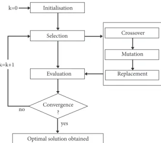
Once the new population is obtained, the process of improving the individuals will be repeated to generate the new population, and so on. The process will be stopped as soon as we no longer observe a substantial evolution of individuals in the current population (this corresponds to a maximum number of generations). At the end of the program, we obtain a population of solutions from which we can extract the most efficient solution (measured by its rank). It is this solution that approaches the global optimum of the studied problem. Figure 3 illustrates the principle of building an GA generation.
3. Application of HySubF-CVFEM/GA
Integrated Optimization Algorithm
Before applying the combination HySubF-CVFEM/GA to identify the real transmissivity field, we first validate this combination on a schematic case offering an analytical solution. This is to solve the following problem:
(𝐼𝑃) { { { { { { { { { { { { { { { { { { { { { { { Minimize K∈Ω𝐴 𝐹 (𝐾) 𝑢𝑛𝑑𝑒𝑟 𝑐𝑜𝑛𝑠𝑡𝑟𝑎𝑖𝑛𝑡𝑠 (𝐷𝑃) { { { { { { { { { −∇. (𝐾∇𝜑) = 𝑆 𝑖𝑛 Ω 𝜑 = 𝜑𝐷 𝑖𝑛 𝜕Ω𝐷 →𝑛 .→𝑞 = 𝜑 𝑁 𝑖𝑛 𝜕Ω𝑁 (28)
k=0 Initialisation Selection Evaluation Crossover Mutation k=k+1 Replacement no Convergence ? yes Optimal solution obtained
Figure 3: The schematic diagram of one generation in GA.
whereΩ𝐴is the admissible set values of the tensor and𝐹 is the objective function given by
𝐹 (K) =𝜑𝑜𝑏𝑠− 𝜑 (𝐾) (29) Figure 4 illustrates the computations sequence of the pro-posed integrated optimization algorithm. The convergence of this algorithm will provide the optimal solution𝐾optwhich is none other than the desired transmissivity fields.
𝐾opt= min
K∈Ω𝐴
𝜑𝑜𝑏𝑠− 𝜑 (𝐾) (30) In addition to the stability problems that the HySubF-CVFEM/GA coupling can generate by the use of the poor accurate solution, it should be noted that the inverse prob-lems can be confronted to the uniqueness solution problem. Indeed, different hydrological configurations can provide identical observations 𝜑𝑜𝑏𝑠. Therefore, it is difficult (if not impossible) to uniquely identify a particular aquifer situation solely from the observations. In Smaoui et al. 2018, the reader will find some methods adopted to ensure the uniqueness of the solution of the inverse problem in hydrogeology.
3.1. Numerical Test (Validation Case). To verify the
perfor-mance of the proposed coupling to identify by optimization the transmissivity fields, we apply this methodology to an inverse problem with an analytical solution. This exercise allows us to validate the HySubF-CVFEM/GA coupling, but also to estimate the error level by evaluating the difference between the analytical and numerical solutions obtained by the developed, integrated optimization model HySubF-CVFEM/GA. It should be noted that we have made com-parisons with the results of other authors [27] solving the inverse problem for real cases by other optimization methods based on gradient methods. These comparisons were made to verify the ability of HySubF-CVFEM/GA
to reproduce the real case solution performed by these authors. It emerges from these comparisons that the HySubF-CVFEM/GA coupling has allowed to obtain the global opti-mal solution with excellent accuracy, but with a convergence speed approaching unity (significant computation time). It should be noted that this validation test was studied by Smaoui et al. [19], but for another integrated optimization algorithm called HySubF-FEM/CMA-ES which differs from the present model both by method solving the direct problem (finite element method) and by the optimization method (CMA-ES: Covariance Matrix Adaptation Evolution Strat-egy) that is based on evolution algorithms. The details of these comparisons are presented in Smaoui et al. [19].
In this paper, we present the results of an inverse problem with an analytical solution. This is the solution of the 2D direct problem on a rectangular domainΩ = [0, a] × [0, b] with a given isotropic transmissivity linear field in the form 𝐾(𝑥, 𝑦) = 𝛼(𝑥 + 𝑦) and Dirichelet boundary condition type. The problem to be solved can be formulated by
(𝐷𝑃){{ {
−∇. (𝐾∇𝜑) = 𝑆 (𝑥, 𝑦) ∈ Ω
𝜑 = 𝜑𝐷 (𝑥, 𝑦) ∈ 𝜕Ω (31) with form𝑆(𝑥, 𝑦) = −6𝛼𝛽(𝑥 + 𝑦) and 𝜑𝐷(𝑥, 𝑦) = 𝜑𝑒𝑥𝑎𝑐𝑡(𝑥, 𝑦) on the domain boundary 𝜕Ω. The exact solution of the problem (31) reads
𝜑𝑒𝑥𝑎𝑐𝑡(𝑥, 𝑦) = 𝛽 (𝑥2+ 𝑦2) (32) It should be remembered that the aim of this exercise is to solve the inverse problem. That is to say, given the solution 𝜑𝑒𝑥𝑎𝑐𝑡is the proposed HySubF-CVFEM/GA able to find the optimal solution? which in this case is exactly the function
𝐾 (𝑥, 𝑦) = [𝑇 (𝑥, 𝑦) 0 0 𝑇 (𝑥, 𝑦)]
𝑤𝑖𝑡ℎ 𝑇 (𝑥, 𝑦) = 𝛼 (𝑥 + 𝑦) . (33)
k=0 Selection Evaluation: Crossover Mutation k=k+1 Replacement no yes
Initialisation Population0 Givenobs
PutK in the Population 0 and remove the weakest individu
-forK, Call HySubF-CVFEM to compute sim -ComputeF(K) = obs− sim‖
F(K) < tol
K is the optimal solution
K
Figure 4: The integrated optimization algorithm (coupling of the HySubF-CVFEM/GA model).
This problem has already been studied by Smaoui et al., [19] with𝑎 = 3500𝑚; 𝑏 = 2000𝑚; 𝛼 = 10−5; 𝛽 = 10−6. With the𝑎 and 𝑏 values, the function 𝑇 is bounded between 0 and 𝛼(𝑎 + 𝑏). These two limit values were useful to use the version of integrated optimization model HySubF-CVFEM/GA with constraints to limit the research space to the admissible values and thus saving time of computation.
It is the algorithm illustrated in Figure 4 that has been applied to this test case. Analysis of simulation results showed that the model has identified the field 𝑇 with excellent accuracy. The 𝐿∞ absolute error is about3.5 × 10−5𝑚2𝑠−1, while the relative error(‖𝑇𝑒𝑥𝑎𝑐𝑡− 𝑇𝑖𝑑𝑒𝑛𝑡𝑖𝑓𝑖𝑒𝑑‖/‖𝑇𝑖𝑑𝑒𝑛𝑡𝑖𝑓𝑖𝑒𝑑‖) does not exceed1%. We also study the behavior of the convergence of the proposed algorithm. Indeed, the evolution curve of the objective function as a function of iteration numbers (not shown here) shows that during the first 2500 generations the value of the objective function is10−3to reach the value 2.1 × 10⁻⁴ for 3200 generations. This observation allows us to conclude that genetic algorithms are relatively fast at the beginning of the research process, but stagnate when we approach convergence. This finding is not surprising and is inherent in the design of the GAs. Indeed, at the beginning of the search stage the AG needs to look for an improvement among a vast population. It is therefore easy to find better solutions of the previous ones. However, as the process progresses, there is a population with only the best solutions. As a result, it becomes difficult to improve the solutions. This translates into a minimal gain in accuracy at the end of the search process. In other words, near convergence, AGs continue to make generations to gain only a few significant digits in precision. The slowness of GA near convergence has already been observed by the several authors using genetic algorithms as optimization tools [28].
Figure 6 summarizes the comparison between the ana-lytical solution𝑇𝑒𝑥𝑎𝑐𝑡 and the numerical solution𝑇𝑖𝑑𝑒𝑛𝑡𝑖𝑓𝑖𝑒𝑑. It presents the identified transmissivity according to the exact transmissivity. On this graph a 1: 1 straight slope curve has been superimposed to assess the absolute difference between the exact solution and the solution identified by our code HySubF-CVFEM/GA. One can see a good agreement between the two solutions. This figure illustrates also that the relative error does not exceed1% as mentioned above. In our opinion the high accuracy of the results obtained for this schematic case is due to the nature of the PDE equation which governs the direct problem (second-order elliptic), but also the schematic case treated by HySubF-CVFEM/GA is an well-posed constrained optimization problem.
3.2. Realistic Case. The coastal aquifers play an important
role in the in the socioeconomic development of the coastal plains. These costal aquifers are particularly exposed to overexploitation problems that can induce aquifer salin-ization. Also, as presented in the Intergovernmental Panel on climate change (IPCC, 2007), climate changes that will provide variations in the sea level, temperature and rate and intensity of precipitation. All these changes will affect freshwater resources, both in terms of quantity and quality [8].
For several decades, observations by hydrogeologists in the Chaouia region (Figure 7) have led to significant drops in the water table, but also with the risk of saline invasion. It is therefore urgent to have a numerical tool capable of simulat-ing the behavior of this aquifer system. It is in this context that we apply the integrated optimization model HySubF-CVFEM/GA to the Chaouia coastal plain located along the Atlantic coast of Morocco. It extends from Casablanca to
2 000 1 500 1 000 500 0 2 000 3 000 3 500 1 500 2 500 1 000 500 0 Γ2 Γ1 1 2 9 10 11 17 18 25 26 33 15 23 31 8 16 24 32 40 Γ3 Γ4
Figure 5: Mesh of the studied domain and internal nodes [19].
3.2 3 2.8 2.6 2.4 2.22.2 2.4 2.6 2.8 3 3.2 (15) (13,22,31) (11,20,29) (14,23) (12,21,30) (18,27) (10,19,28) (26) 4iden tified (m 2 /s) 4?R;=N(m2/s)
Figure 6: Exact versus identified transmissivity with a line of 1:1slope. Values in parentheses indicate the node number of the mesh plotted in Figure 5 [19]. W N E S 0 10 20
Kilometers Limit of the study area
Azemmour over a distance of65𝑘𝑚 and a width of 15 to 20𝑘𝑚 corresponding to a surface of about1100𝑘𝑚2[29]. This area represents a fairly flat surface with only a few sandy dunes parallel to the Atlantic Ocean (See Figure 7 for location). The Chaouia coastal aquifer constitutes an important aquifer in west Morocco where the irrigated agriculture farming is the main economic resource of the region. This aquifer is subject to intensive water pumping and water quality deterioration by salinization. For these raisons, the hydrogeological modeling became an important way to evaluate water resource and quality for aquifers management. The HySuf-CVFEM/GA code is used to identify the transmissivity field of the Chaouia costal aquifer.
Based on the geological formation, groundwater in the Chaouia aquifer exists from place to place in the Paleozoic schist, in the Cretaceous or in the Plio-Quaternary formation and for each aquifer, the thickness is included between 5 and 20𝑚 (Mostadraf et al., 2008). It is important to recall that there are vertical and horizontal hydraulic communica-tions between these aquifers. Different pumping tests were performed in the studied area with the objective to evaluate the aquifer transmissivity. The obtained values are included between10−5𝑚2𝑠−1and3.62 × 10−2𝑚2𝑠−1and the mean value corresponds to 2.62 × 10⁻²𝑚2𝑠−1. Otherwise piezometric maps of the Chaouia coastal aquifer were performed by different authors showing that the water flow is uniformly directed towards the Atlantic Ocean except in the southern part of the groundwater where the water flows from the East to the West.
It should be noted that the numerical model HySuf-CVFEM was validated for hydrodynamics by comparison with analytical solution, then by comparison with the results of other numerical model massively used in modeling of the underground flows. The analysis of the results of the compar-isons showed that the model HySuf-CVFEM reproduces with a good precision the flow studied. From these comparisons, it was also concluded that our numerical model provides good mass conservation which is a fundamental property in fluid flow. The results of these comparisons are not presented in this paper, but can be found in Smaoui et al., [26]
The chosen area for HySuf-CVFEM/GA model applica-tion is extended to an area about800𝑘𝑚2. It is limited by the Atlantic Ocean at the North-West, the Oum-Erbia river at the South-West, the El Hank at the North-East and the Berrechid plain to the South-East (Figure 7). Taking into account the real geometry of the aquifer and its hydrogeological characteristics, we have constructed a numerical model of the Chaouia aquifer discretized in triangular mesh of 5100 nodes and 9922 elements. For boundary conditions, we have adopted the following conditions. We impose the condition of zero flux (Neumann condition) along El Hank at north-east and at along the streamline connecting the upstream limit to the Oum-Erbia river. On the Atlantic coastline we have imposed a head (Dirichlet condition) corresponding to the sea level which constitutes a natural outflow of the water table. Finally, at the Berrechid plain and Oum-Erbia river mixed boundary condition was imposed depending on a given load. To complete the data necessary for the calculation process,
we have estimated the recharge that is done by infiltration of rainwater. This recharge corresponds to15% of the rainfall. The effective rainfall was thus calculated using daily precip-itation to obtain1.62 × 10−9ms−1per triangular element. To complete the data necessary for the calculation, infiltration values were estimated from the daily water balance, which were computed using the Thornthwaite method. The effective rainfall was thus calculated using daily precipitation to obtain 12.6 × 10⁻³m3s−1per triangular element.
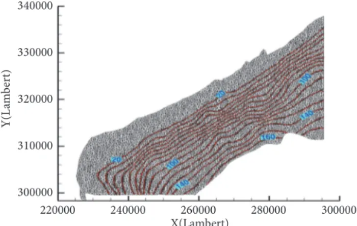
3.3. Results Interpretation and Discussion. Calculated (red)
and measured (blue) piezometric level are presented in Figure 8. This last figure shows a perfect agreement between the two piezometric levels. The difference between these two values does not exceed 2 m at the 160 m and the relative error is about 1.0%. Considering the measurement errors of the piezometric levels that are related to the wells elevations and to water depths, these differences can be considered as acceptable.
The calculated transmissivity using the proposed code is shown in Figure 9. This figure indicates that the obtained transmissivity has a heterogeneous distribution over the studied area. These calculated values of this hydrogeological parameter are included between 10−5and 10−2m2/s.
Based on this transmissivity distribution, two distin-guished areas can be identified:
(i) the first one, with high transmissivity that can reach the values higher than 10−2m2/s; these are located: (i) around and in the north coastal area of the Bir jdid city and (ii) around Oum Rbia river;
(ii) the second areas with lower transmissivity values (lower than 2.10−3m2/s) are located in the interme-diate zone between coastal area and south part of the studied area.
Different factors can explain the transmissivity distribution in the studied area:
(i) The aquifer lithology: the higher transmissivity values are related to Pliocene and Quaternary formations; however, the lower transmissivity is related to pres-ence of Cenomanian marly-limestone formation in the southwest of the studied are and to Palaeozoic bedrock formation in the east part of studied area; (ii) The aquifers thickness which are included between 5
and 20 m [30].
Finally, it is important to recall that the calculated values are in the same range than those obtained using pumped test.
4. Conclusions
Most of the hydrogeological parameter identification prob-lems have been formulated and solved by gradient optimiza-tion methods. These methods may prove unusable when the objective function is not regular enough. In addition, when convergence towards the optimum is ensured, this type of method generally converges towards a local optimum.
340000 330000 320000 310000 300000 220000 240000 260000 280000 300000 X(Lambert) Y(L am b er t)
Figure 8: Head comparison: measured and computed from the HySuf-CVFEM/GA model. (red line= measures, black line= computation).
340000 330000 320000 310000 300000 220000 240000 260000 280000 300000 X(Lambert) Y(L am b er t) 10 20 30 40 50 60 70 80 90 100 110
Figure 9: Identified transmissivity field of Chaouia aquifer by HySuf-CVFEM/GA model. (values must be multiplied by 10−7factor).
In recent years we have been witnessing the emergence of metaheuristic optimization methods and, more specifically, genetic algorithms (GA). On one hand, this type of method does not require a minimum of regularity of the objective function; on the other hand, these methods converge towards a global minimum. This paper deals with solving the inverse problem by coupling two computation codes: the first is the HySuF-CVFEM code to solve the direct problem and the second is the code of the genetic algorithm to solve the optimization problem. Our choice was for the GA for the optimization phase is for not only to focus on demon-strating the regularity of the objective function, but also to ensure convergence towards a global optimum. The proposed HySuF-CVFEM/GA integrated optimization algorithm has been validated by comparison with analytical solutions. This comparison showed that the code thus constructed HySuF-CVFEM/GA is able to provide (by identification) a real transmissivity field of excellent quality. This coupling method has also been applied to the real case of the coastal aquifer of the “Chaouia” region in Western Morocco and has identified complex domains characterizing the heterogeneity of this aquifer. Nevertheless, it should be noted that the major disadvantage of HySuF-CVFEM/GA coupling remains the longer time required to reach convergence towards the global optimum. To avoid this inconvenience, we plan to use
parallel computing techniques for HySuF-CVFEM/GA cou-pling. Similarly, we will consider GA coupling with Kriging methods that are beginning to emerge in the identification parameters in hydrogeological research. Another interesting way is to attempt model reduction techniques to reduce the number of components of the variable vector. These tech-niques will be based on orthogonal decomposition (POD) and properly generalized decomposition (PGD) methods.
Data Availability
The data used to support the findings of this study are available from the corresponding author upon request.
Conflicts of Interest
The authors declare that they have no conflicts of interest.
Acknowledgments
The authors wish to thank the anonymous reviewers for their constructive criticism that led to the improvement of the manuscript.
References
[1] J. F. Carneiro, M. Boughriba, A. Correia, Y. Zarhloule, A. Rimi, and B. El Houadi, “Evaluation of climate change effects in a coastal aquifer in Morocco using a density-dependent numerical model,” Environmental Earth Sciences, vol. 61, no. 2, pp. 241–252, 2010.
[2] Y. Fakir, A. Zerouali, M. Aboufirassi, and M. Bouabdelli, “Exploitation et salinit´e des aquif`eres de la Chaouia cˆoti`ere, littoral atlantique,” Journal of African Earth Sciences, vol. 32, no. 4, pp. 791–801, 2001.
[3] Y. Fakir and M. Razack, “Hydrodynamic characterization of a Sahelian coastal aquifer using the ocean tide effect (Dridrate Aquifer, Morocco),” Hydrological Sciences Journal, vol. 48, no. 3, pp. 441–454, 2003.
[4] B. Benseddik, E. El Mrabet, B. El Mansouri, J. Chao, and M. Kili, “Delineation of artificial recharge zones in Mnasra Aquifer (NW, Morocco),” Modeling Earth Systems and Environment, vol. 4, pp. 3–10, 2017.
[5] A. D. Koussis, K. Mazi, and G. Destouni, “Analytical single-potential, sharp-interface solutions for regional seawater intru-sion in sloping unconfined coastal aquifers, with pumping and recharge,” Journal of Hydrology, vol. 416-417, pp. 1–11, 2012. [6] A. D. Koussis and K. Mazi, “Corrected interface flow model
for seawater intrusion in confined aquifers: relations to the dimensionless parameters of variable-density flow,” Hydrogeol-ogy Journal, vol. 26, no. 8, pp. 2547–2559, 2018.
[7] P. M. Carreira, M. Bahir, O. Salah, P. Galego Fernandes, and D. Nunes, “Correction: Tracing salinization processes in coastal aquifers using an isotopic and geochemical approach: com-parative studies in western Morocco and southwest Portugal,” Hydrogeology Journal, vol. 26, no. 8, p. 2933, 2018.
[8] B. C. Bates, Z. W. Kundzewicz, S. Wu, and J. P. Palutikof, Tech-nical Paper on Climate Change and Water, IPCC, Cambridge University Press, Cambridge, UK, 2008.
[9] P. O. Yapo, H. V. Gupta, and S. Sorooshian, “Multi-objective global optimization method for hydrological models,” Journal of Hydrologie, vol. 204, pp. 204-83, 1998.
[10] J. Morshed and J. J. Kaluarachchi, “Application of artificial neural network and genetic algorithm in flow and transport simulations,” Advances in Water Resources, vol. 22, no. 2, pp. 145–158, 1998.
[11] D. K. Karpouzos, F. Delay, K. L. Katsifarakis, and G. De Marsily, “A multipopulation genetic algorithm to solve the inverse problem in hydrogeology,” Water Resources Research, vol. 37, no. 9, pp. 2291–2302, 2001.
[12] Q. Duan, J. Schaake, V. Andr´eassian et al., “Model Parameter Estimation Experiment (MOPEX): an overview of science strat-egy and major results from the second and third workshops,” Journal of Hydrology, vol. 320, no. 1-2, pp. 3–17, 2006.
[13] K. C. Abbaspour, C. A. Johnson, and M. T. van Genuchten, “Estimating uncertain flow and transport parameters using a sequential uncertainty fitting procedure,” Vadose Zone Journal, vol. 3, no. 4, pp. 1340–1352, 2004.
[14] M. H. Tber, M. El Alaoui Talibi, and D. Ouazar, “Parameters identification in a seawater intrusion model using adjoint sensitive method,” Mathematics and Computers in Simulation, vol. 77, no. 2-3, pp. 301–312, 2007.
[15] K. A. Tapesh and A. K. Rastogi, “Artificial neural network application on estimation of aquifer transmissivity,” Journal of Spatial Hydrology, vol. 8, no. 2, pp. 15–31, 2008.
[16] H. Hashemi, R. Berndtsson, M. Kompani-Zare, and M. Persson, “Natural vs. artificial groundwater recharge, quantification through inverse modeling,” Hydrology and Earth System Sci-ences, vol. 17, no. 2, pp. 637–650, 2013.
[17] W. W.-G. Yeh, “Review of parameter identification proce-dures in groundwater hydrology: the inverse problem,” Water Resources Research, vol. 22, no. 2, pp. 95–108, 1986.
[18] J. Carrera, “State of the art of the inverse problem applied to the flow and solute transport equations,” in Groundwater Flow and Quality Modelling, E. Custodio, A. Gurgui, and J. P. Ferreira, Eds., vol. 224 of NATO ASI Series (Series C: Mathematical and Physical Sciences), pp. 549–583, Springer, Dordrecht, Netherlands, 1988.
[19] H. Smaoui, L. Zouhri, S. Kaidi, and E. Carlier, “Combination of FEM and CMA-ES algorithm for transmissivity identification in aquifer systems,” Hydrological Processes, vol. 32, no. 2, pp. 264– 277, 2018.
[20] J. Moustadraf, Mod´elisation num´erique d’un syst`eme aquif`ere cˆotier : Etude de l’impact de la s´echeresse et de l’intrusion marine. La Chaouia Cˆoti`ere, Maroc, Th`ese de Doctorat de l’Universit´e de Poitiers, France, 2006.
[21] P. G. Ciarlet, “The finite element method for elliptic problems,” in Classics in Applied Mathematics, p. 530, SIAM, Philadelphia, Pa, USA, 1978.
[22] R. Huber and R. Helmig, “Node-centered finite volume dis-cretizations for the numerical simulation of multiphase flow in heterogeneous porous media,” Computational Geosciences, vol. 4, no. 2, pp. 141–164, 2000.
[23] G. Manzini and S. Ferraris, “Mass-conservative finite volume methods on 2-D unstructured grids for the Richards’ equation,” Advances in Water Resources, vol. 27, no. 12, pp. 1199–1215, 2004. [24] B. R. Baliga and S. V. Patankar, “A new finite-element for-mulation for convection-diffusion problems,” Numerical Heat Transfer, vol. 3, no. 4, pp. 393–409, 1980.
[25] B. R. Baliga and S. V. Patankar, “A control volume finite-element method for two-dimensional fluid flow and heat transfer,” Numerical Heat Transfer, vol. 6, no. 3, pp. 245–261, 1983. [26] H. Smaoui, L. Zouhri, and S. Kaidi, “Parameters identification
in hydrogeology by using the CMA-ES algorithm,” Research Report No 2015.1, Cerema /DTecEMF, Compi`egne, France, 2015.
[27] F. T.-C. Tsai, N.-Z. Sun, and W. W.-G. Yeh, “A combinatorial optimization scheme for parameter structure identification in ground water modeling,” Groundwater, vol. 41, no. 2, pp. 156– 169, 2003.
[28] S. Baluja, “Structure and performance of fine Frain parallelism in genetic search,” in Practical Handbook of Genetic Algorithms, L. Chmabers, Ed., vol. 2, pp. 139–154, New Frontiers, Boca Raton, Fla, USA, 1995.
[29] A. Marjoua, P. Olive, and C. Jusserand, “Apports des outils chimiques et isotopiques `a l’identification des origines de la salinisation des eaux : Cas de la nappe de La Chaouia cˆoti`ere (Maroc),” Journal of Water Science, vol. 10, no. 4, pp. 489–505, 1997.
[30] A. Marjoua, Approche g´eochimique et mod´elisation hydrody-namique de l’aquif`ere de la Chaouia Cˆoti`ere (Maroc) : Origines de la salinisation des eaux, Th`ese de doctorat de l’universit´e Paris VI, France, 1995.
Hindawi www.hindawi.com Volume 2018
Mathematics
Journal of Hindawi www.hindawi.com Volume 2018 Mathematical Problems in Engineering Applied Mathematics Hindawi www.hindawi.com Volume 2018Probability and Statistics Hindawi
www.hindawi.com Volume 2018
Hindawi
www.hindawi.com Volume 2018
Mathematical PhysicsAdvances in
Complex Analysis
Journal ofHindawi www.hindawi.com Volume 2018
Optimization
Journal of Hindawi www.hindawi.com Volume 2018 Hindawi www.hindawi.com Volume 2018 Engineering Mathematics International Journal of Hindawi www.hindawi.com Volume 2018 Operations Research Journal of Hindawi www.hindawi.com Volume 2018Function Spaces
Abstract and Applied AnalysisHindawi www.hindawi.com Volume 2018 International Journal of Mathematics and Mathematical Sciences Hindawi www.hindawi.com Volume 2018
Hindawi Publishing Corporation
http://www.hindawi.com Volume 2013 Hindawi www.hindawi.com
World Journal
Volume 2018 Hindawiwww.hindawi.com Volume 2018Volume 2018
Numerical Analysis
Numerical Analysis
Numerical Analysis
Numerical Analysis
Numerical Analysis
Numerical Analysis
Numerical Analysis
Numerical Analysis
Numerical Analysis
Numerical Analysis
Numerical Analysis
Numerical Analysis
Advances inAdvances in Discrete Dynamics in Nature and SocietyHindawi www.hindawi.com Volume 2018 Hindawi www.hindawi.com Differential Equations International Journal of Volume 2018 Hindawi www.hindawi.com Volume 2018


![Figure 7: Location of the Chaouia coastal aquifer [20].](https://thumb-eu.123doks.com/thumbv2/123doknet/7640669.236549/11.900.136.762.718.1052/figure-location-chaouia-coastal-aquifer.webp)