Projection-Based Statistical Inference in Linear Structural Models with Possibly Weak Instruments

Texte intégral

(1)2003s-39. Projection-Based Statistical Inference in Linear Structural Models with Possibly Weak Instruments Jean-Marie Dufour, Mohamed Taamouti. Série Scientifique Scientific Series. Montréal Mai 2003. © 2003 Jean-Marie Dufour, Mohamed Taamouti. Tous droits réservés. All rights reserved. Reproduction partielle permise avec citation du document source, incluant la notice ©. Short sections may be quoted without explicit permission, if full credit, including © notice, is given to the source..

(2) CIRANO Le CIRANO est un organisme sans but lucratif constitué en vertu de la Loi des compagnies du Québec. Le financement de son infrastructure et de ses activités de recherche provient des cotisations de ses organisationsmembres, d’une subvention d’infrastructure du ministère de la Recherche, de la Science et de la Technologie, de même que des subventions et mandats obtenus par ses équipes de recherche. CIRANO is a private non-profit organization incorporated under the Québec Companies Act. Its infrastructure and research activities are funded through fees paid by member organizations, an infrastructure grant from the Ministère de la Recherche, de la Science et de la Technologie, and grants and research mandates obtained by its research teams. Les organisations-partenaires / The Partner Organizations PARTENAIRE MAJEUR . Ministère du développement économique et régional [MDER] PARTENAIRES . Alcan inc. . Axa Canada . Banque du Canada . Banque Laurentienne du Canada . Banque Nationale du Canada . Banque Royale du Canada . Bell Canada . Bombardier . Bourse de Montréal . Développement des ressources humaines Canada [DRHC] . Fédération des caisses Desjardins du Québec . Gaz Métropolitain . Hydro-Québec . Industrie Canada . Ministère des Finances [MF] . Pratt & Whitney Canada Inc. . Raymond Chabot Grant Thornton . Ville de Montréal . École Polytechnique de Montréal . HEC Montréal . Université Concordia . Université de Montréal . Université du Québec à Montréal . Université Laval . Université McGill ASSOCIÉ AU : . Institut de Finance Mathématique de Montréal (IFM2) . Laboratoires universitaires Bell Canada . Réseau de calcul et de modélisation mathématique [RCM2] . Réseau de centres d’excellence MITACS (Les mathématiques des technologies de l’information et des systèmes complexes) Les cahiers de la série scientifique (CS) visent à rendre accessibles des résultats de recherche effectuée au CIRANO afin de susciter échanges et commentaires. Ces cahiers sont écrits dans le style des publications scientifiques. Les idées et les opinions émises sont sous l’unique responsabilité des auteurs et ne représentent pas nécessairement les positions du CIRANO ou de ses partenaires. This paper presents research carried out at CIRANO and aims at encouraging discussion and comment. The observations and viewpoints expressed are the sole responsibility of the authors. They do not necessarily represent positions of CIRANO or its partners.. ISSN 1198-8177.

(3) Projection-Based Statistical Inference in Linear Structural Models with Possibly Weak Instruments * Jean-Marie Dufour†, Mohamed Taamouti‡ Résumé / Abstract L’une des questions les plus étudiées récemment en économétrie est celle des modèles présentant des problèmes de quasi non-identification ou d’instruments faibles. L’une des conséquences importantes de ce problème est la non validité de la théorie asymptotique standard [Dufour (1997, Econometrica), Staiger et Stock (1997, Econometrica), Wang et Zivot (1998, Econometrica), Stock et Wright (2000, Econometrica), Dufour et Jasiak (2001, International Economic Review)]. Le défi majeur dans ce cas consiste à trouver des méthodes d’inférence robustes à ce problème. Une solution possible consiste à utiliser la statistique d’Anderson-Rubin (1949, Ann. Math. Stat.). Nous mettons l’emphase sur les procédures de type Anderson-Rubin, car celles-ci sont robustes tant à la présence d’instruments faibles et à l’exclusion d’instruments. Cette dernière ne fournit cependant des tests exacts que pour les hypothèses spécifiant le vecteur entier des coefficients des variables endogènes dans un modèle structurel, et de façon correspondante, que des régions de confiance simultanées pour ces coefficients. Elle ne permet pas de tester des hypothèses spécifiant des coefficients individuels ou sur des transformations de ces coefficients. Ce problème peut être résolu en principe par des techniques de projection [Dufour (1997, Econometrica), Dufour et Jasiak (2001, International Economic Review)]. Cependant , ces techniques ne sont pas toujours faciles à appliquer et requièrent en général l’emploi de méthodes numériques. Dans ce texte, nous proposons une solution explicite complète au problème de la construction de régions de confiance par projection basées sur des statistiques de type Anderson-Rubin. Cette solution exploite les propriétés géométriques des “quadriques” et peut s’interpréter comme une extension des intervalles et ellipsoïdes de confiance usuels. Le calcul de ces régions ne requièrent que des techniques de moindres carrés. Nous étudions également par simulation le degré de conservatisme des régions de confiance obtenues par projection. Enfin, nous illustrons les méthodes proposées par trois applications différentes: la relation entre l’ouverture commerciale et la croissance, le rendement de l’éducation et une étude sur les rendement d’échelles dans l’économie américaine. Mots clés : équations simultanées ; modèle structurel ; variable instrumentale; instruments faibles; intervalle de confiance ; test ; projection ; inférence simultanée ; inférence exacte; théorie asymptotique. *. The authors thank Craig Burnside for providing us his data, as well as Laurence Broze, John Cragg, Jean-Pierre Florens, Christian Gouriéroux, Joanna Jasiak, Frédéric Jouneau, Lynda Khalaf, Nour Meddahi, Benoît Perron, Tim Vogelsang and Eric Zivot for several useful comments. This work was supported by the Canada Research Chair Program (Chair in Econometrics, Université de Montréal), the Alexander-von-Humboldt Foundation (Germany), the Canadian Network of Centres of Excellence [program on Mathematics of Information Technology and Complex Systems (MITACS)], the Canada Council for the Arts (Killam Fellowship), the Natural Sciences and Engineering Research Council of Canada, the Social Sciences and Humanities Research Council of Canada, the Fonds de recherche sur la société et la culture (Québec), and the Fonds de recherche sur la nature et les technologies (Québec). One of the authors (Taamouti) was also supported by a Fellowship of the Canadian International Development Agency (CIDA). † Canada Research Chair Holder (Econometrics). Centre interuniversitaire de recherche en analyse des organisations (CIRANO), Centre interuniversitaire de recherche en économie quantitative (CIREQ), and Département de sciences économiques, Université de Montréal. Mailing address: Département de sciences économiques, Université de Montréal, C.P. 6128 succursale Centre-ville, Montréal, Québec, Canada H3C 3J7. Tel: 1 514 343 2400; Fax: 1 514 343 5831; e-mail: jean.marie.dufour@umontreal.ca. Web page: http://www.fas.umontreal.ca/SCECO/Dufour . ‡ INSEA, Rabat and CIREQ, Université de Montréal. Mailing address: INSEA., B.P. 6217, Rabat-Instituts, Rabat, Morocco. Tel: 212 7 77 09 26; Fax: 212 7 77 94 57. e-mail: taamouti@insea.ac.ma..

(4) It is well known that standard asymptotic theory is not valid or is extremely unreliable in models with identification problems or weak instruments [Dufour (1997, Econometrica), Staiger and Stock (1997, Econometrica), Wang and Zivot (1998, Econometrica), Stock and Wright (2000, Econometrica), Dufour and Jasiak (2001, International Economic Review)]. One possible way out consists here in using a variant of the Anderson-Rubin (1949, Ann. Math. Stat.) procedure. The latter, however, allows one to build exact tests and confidence sets only for the full vector of the coefficients of the endogenous explanatory variables in a structural equation, which in general does not allow for individual coefficients. This problem may in principle be overcome by using projection techniques [Dufour (1997, Econometrica), Dufour and Jasiak (2001, International Economic Review)]. Artypes are emphasized because they are robust to both weak instruments and instrument exclusion. However, these techniques can be implemented only by using costly numerical techniques. In this paper, we provide a complete analytic solution to the problem of building projection-based confidence sets from Anderson-Rubin-type confidence sets. The latter involves the geometric properties of “quadrics” and can be viewed as an extension of usual confidence intervals and ellipsoids. Only least squares techniques are required for building the confidence intervals. We also study by simulation how “conservative” projection-based confidence sets are. Finally, we illustrate the methods proposed by applying them to three different examples: the relationship between trade and growth in a crosssection of countries, returns to education, and a study of production functions in the U.S. economy. Keyswords : Simultaneous equations; structural model; instrumental variable; weak instrument; confidence interval; testing; projection; simultaneous inference; exact inference; asymptotic theory..

(5) Contents List of Propositions and Theorems. iv. 1.. Introduction. 1. 2.. Framework. 4. 3.. Quadric confidence sets. 7. 4.. 5.. 6. 7.. Geometry of quadric confidence sets 4.1. Nonsingular concentration matrix . . . . . . . . . . . . . . . . . . . 4.1.1. Positive definite concentration matrix . . . . . . . . . . . . . 4.1.2. Negative definite concentration matrix . . . . . . . . . . . . 4.1.3. Concentration matrix not positive or negative definite . . . . 4.2. Singular concentration matrix . . . . . . . . . . . . . . . . . . . . . 4.3. Necessary and sufficient condition for bounded quadric confidence set 4.4. Joint confidence sets for β and γ . . . . . . . . . . . . . . . . . . . Confidence sets for transformations of β 5.1. The projection approach . . . . . . . . . . . . . . . . . . . . . 5.2. Projection-based confidence sets for scalar linear transformations 5.2.1. Nonsingular concentration matrix . . . . . . . . . . . . . 5.2.2. Singular concentration matrix . . . . . . . . . . . . . . . 5.3. A Wald-type interpretation of the projection-based confidence sets. . . . . .. . . . . .. . . . . . . . . . . . .. . . . . . . . . . . . .. . . . . . . . . . . . .. . . . . . . . . . . . .. . . . . . . . . . . . .. . . . . . . .. 9 9 10 10 10 11 11 12. . . . . .. 12 12 13 14 16 18. Monte Carlo evaluation. 19. Empirical illustrations 7.1. Trade and growth . . . . . . . . . . . . . . . . . . . . . . . . . . . . . . . . . 7.2. Education and earnings . . . . . . . . . . . . . . . . . . . . . . . . . . . . . . 7.3. Returns to scale and externality spillovers in U.S. industry . . . . . . . . . . . .. 29 29 32 34. 8.. Conclusion. 36. A.. Appendix: Proofs. 38. iii.

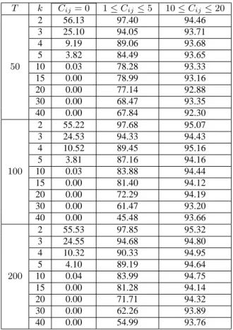
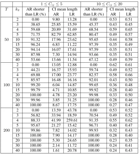
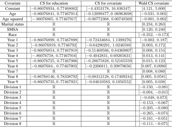
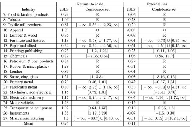
(6) List of Propositions and Theorems Theorem : Necessary and sufficient condition for bounded confidence set . . . . . . Theorem : Projection-based confidence sets for linear transformations when the concentration matrix is positive definite . . . . . . . . . . . . . . . . . . . . . . . Corollary : Projection-based confidence interval for an individual coefficient . . . . Theorem : Projection-based confidence sets for linear transformations when the concentration matrix has one negative eigenvalue . . . . . . . . . . . . . . . . . . Theorem : Projection-based confidence sets for linear transformations when the concentration matrix has more than one negative eigenvalue . . . . . . . . . . . . . Theorem : Projection-based confidence sets with a posssibly sigular concentration matrix Proof of equation (4.13) . . . . . . . . . . . . . . . . . . . . . . . . . . . . . . Proof of Theorem 4.1 . . . . . . . . . . . . . . . . . . . . . . . . . . . . . . . Proof of Theorem 5.1 . . . . . . . . . . . . . . . . . . . . . . . . . . . . . . . Proof of Theorem 5.3 . . . . . . . . . . . . . . . . . . . . . . . . . . . . . . . Proof of Theorem 5.4 . . . . . . . . . . . . . . . . . . . . . . . . . . . . . . . Proof of Theorem 5.5 . . . . . . . . . . . . . . . . . . . . . . . . . . . . . . .. 4.1 5.1 5.2 5.3 5.4 5.5. 12 14 14 15 15 17 38 38 38 39 40 40. List of Tables 1 2 3 4 5 6 7 8 9. Empirical coverage rate of TSLS-based Wald confidence sets . . . . . . . . . . . Characteristics of AR projection-based confidence sets _ Cij = 0 . . . . . . . . . Characteristics of AR projection-based confidence sets _1 ≤ Cij ≤ 5 . . . . . . . Characteristics of AR projection-based confidence sets _10 ≤ Cij ≤ 20 . . . . . Comparison between AR and LR projection-based confidence sets when they are bounded . . . . . . . . . . . . . . . . . . . . . . . . . . . . . . . . . . . . . . Power of tests induced by projection-based confidence sets _ H0 : β 1 = 0 . . . . Confidence sets for the coefficients of the Frankel-Romer income-trade equation . Projection-based confidence sets for the coefficients of the exogenous covariates in the income-education equation . . . . . . . . . . . . . . . . . . . . . . . . . . . Confidence sets for the returns to scale and externality coefficients in different U.S. industries . . . . . . . . . . . . . . . . . . . . . . . . . . . . . . . . . . . . . .. 20 21 23 25 27 28 32 34 36. List of Figures 1. Power of tests induced by projection-based confidence sets _ H0 : β 1 = 0.5 . . .. iv. 30.

(7) 1. Introduction One of the classic problems of econometrics consists in making inference on the coefficients of structural models. Such models typically involve endogenous explanatory variables (which can lead to endogeneity biases), the need to use instrumental variables, and the possibility that “structural parameters of interest” may not be identifiable. Recently, the statistical problems raised by structural modelling have received new attention in view of the observation that proposed instruments are often “weak”, i.e. poorly correlated with the relevant endogenous variables, which correspond to situations where the structural parameters are close to being not identifiable (through the instruments used). The literature on so-called “weak instruments” problems is now considerable; see, for example, Nelson and Startz (1990a, 1990b), Buse (1992), Maddala and Jeong (1992), Bound, Jaeger, and Baker (1993, 1995), Angrist and Krueger (1995), Hall, Rudebusch, and Wilcox (1996), Dufour (1997), Shea (1997), Staiger and Stock (1997), Wang and Zivot (1998), Zivot, Startz, and Nelson (1998), Startz, Nelson, and Zivot (1999), Perron (1999), Chao and Swanson (2000), Hall and Peixe (2000), Stock and Wright (2000), Dufour and Jasiak (2001), Hahn and Hausman (2002a, 2002b), Kleibergen (2001, 2002), Moreira (2001, 2002), Stock and Yogo (2002) and Stock, Wright, and Yogo (2002)]. In such contexts, several papers have documented by simulation and approximate asymptotic methods the poor performance of standard asymptotically justified procedures [Nelson and Startz (1990a, 1990b), Buse (1992), Bound, Jaeger, and Baker (1993, 1995), Hall, Rudebusch, and Wilcox (1996), Staiger and Stock (1997), Zivot, Startz, and Nelson (1998), Dufour and Jasiak (2001)]. The main difficulty here is that the finite-sample distributions of the relevant statistics (in particular, test statistics) are very sensitive to unknown nuisance parameters; indeed, they can exhibit an arbitrary large sensitivity to such parameters. Further, limiting distributions are non-standard when identification conditions do not hold, while usual large-sample approximations do not converge uniformly, so that the latter may be arbitrarily inaccurate in finite samples even when identification and standard regularity conditions obtain. The fact that standard asymptotic theory can be arbitrarily inaccurate in finite samples (of any size) is shown rigorously in Dufour (1997), where it is observed that valid confidence intervals in a standard linear structural equations model must be unbounded with positive probability and Wald-type statistics have distributions which can deviate arbitrarily from their large-sample distribution (even when identification holds). The fact that both finite-sample and large-sample distributions exhibit strong dependence upon nuisance parameters has also been demonstrated by other methods, such as finite-sample distributional theory [see Choi and Phillips (1992)] and local to nonidentification asymptotics [see Staiger and Stock (1997) and Wang and Zivot (1998)]. As a result, it appears especially important in such problems to build tests and confidence sets based on properly pivotal (or boundedly pivotal) functions, as well as to study inference procedures from a finite-sample perspective. The fact that tests should be based on statistics whose distributions can be bounded and that confidence sets should be obtained from pivotal statistics is, of course, a requirement of basic statistical theory [see Lehmann (1986)]. In the framework of linear simultaneous equations and in view of weak instrument problems, the importance of using pivotal functions for statistical inference has been recently reemphasized by several authors [see Dufour (1997), Staiger. 1.

(8) and Stock (1997), Wang and Zivot (1998), Zivot, Startz, and Nelson (1998), Startz, Nelson, and Zivot (1999), Dufour and Jasiak (2001), Stock and Wright (2000), Kleibergen (2001, 2002), Moreira (2001, 2002), and Stock, Wright, and Yogo (2002)]. In particular, this suggests that confidence sets should be built by inverting likelihood ratio (LR) and Lagrange multiplier (LM) type statistics, as opposed to the more usual method which consists in inverting Wald-type statistics (such as asymptotic t-ratios). In this paper, we wish to concentrate on procedures for which finite-sample pivotality obtains under standard assumptions. In view of the results in Dufour (1997), we consider this approach as the best guide to selecting test and confidence set procedures (even though asymptotic validity will hold under weaker distributional assumptions). Useful pivotal functions are however difficult to find in structural models. The oldest one appears to be the statistic proposed by Anderson and Rubin (1949, henceforth AR). The latter is a limited-information method which allows one to test an hypothesis setting the value of the full vector of the endogenous explanatory variable coefficients in a linear structural equation; under usual parametric assumptions (error Gaussianity, instrument strict exogeneity) the distribution of the statistic is a central Fisher distribution, while under weaker (standard) assumptions it is asymptotically chi-square, irrespective of the presence of weak instruments. Limited-information methods typically involve an efficiency loss with respect to full-information methods, but do allow for a less complete specification of the model and more robustness. Indeed, the AR statistic enjoys several remarkable invariance (or robustness) properties. Namely it is completely robust (in finite samples) to the presence of weak instruments (robustness to weak instruments), to the exclusion of possibly relevant instruments (robustness to instrument exclusion), and more generally to the distribution of explanatory endogenous variables (robustness to endogenous explanatory variable distribution).1 More precisely, its finite-sample distribution (under the null hypothesis) is completely unaffected by the presence of “weak instruments”, the exclusion of relevant instruments, and the error distribution in the reduced form for the explanatory endogenous variables. We view all these features as important because it is typically difficult to know whether a set of instruments is globally weak (so that the resulting inference becomes unreliable) or whether relevant instruments have been excluded (which seems highly likely in most practical situations). As a result, tests and confidence sets based on the AR statistic remains valid irrespective whether instruments are weak or relevant instruments have been excluded. Extensions of the AR statistics with the same basic robustness properties and a finite-sample distributional theory are also proposed in Dufour and Jasiak (1993, 2001). Other potential pivots aimed at being robust to weak instruments have recently been suggested by Wang and Zivot (1998), Kleibergen (2002) and Moreira (2002). These methods are closer to being full-information methods _ in the sense that they rely on a relatively specific formulation of the model for the endogenous explanatory variables of the model _ and thus may lead to power gains under the assumptions considered. But this will typically be at the expense of robustness. Further, only asymptotic distributional theories have been supplied for these statistics, so that the level of the procedures may not be controlled in finite samples. Indeed, it is easy to see that none of these 1. We borrow the terminology “robust to weak instruments” from Stock, Wright, and Yogo (2002, p. 518). Robustness to instrument exclusion appears to have been little discussed in the literature on weak instruments.. 2.

(9) statistics is pivotal in finite samples (i.e., their finite-sample distributions involve unknown nuisance parameters) or robust to the exclusion of relevant instruments. It is clear that these statistics do not qualify as pivotal in finite samples. An important practical shortcoming of the above methods is that they are designed to test hypotheses of the form H0 : β = β 0 , where β is the coefficient vector for all the endogenous explanatory variables. In particular these statistics do not allow to test linear and nonlinear restrictions on the vector β. A general solution to this problem is the projection technique described in Dufour (1990, 1997), Wang and Zivot (1998) and Dufour and Jasiak (2001).2 This problem was also considered by Choi and Phillips (1992), Stock and Wright (2000) and Kleibergen (2001). While Choi and Phillips (1992) did not propose an operational method for dealing with the problem, the methods considered by Stock and Wright (2000) and Kleibergen (2001) rely on the assumption that the structural parameters not involved in the restrictions are well identified and rely on largesample approximations (which become invalid when the identification assumptions made do not hold). Consequently they are not robust to weak instruments. For these reasons, we shall focus here on the projection approach. The basic idea behind the projection technique is simple. Let θ be a multidimensional parameter vector for which we can build a confidence set Cθ (α) with level 1 − α : P[θ ∈ Cθ (α)] ≥ 1 − α. Now consider a transformation of interest g(θ) which takes its values in Rm . For example, g(θ) could be one of the components of θ. Then it is easy to see that the image set g[Cθ (α)] ¤= {g(θ) ∈ £ m R : θ ∈ Cθ (α)} is a confidence set with level 1 − α for g(θ), i.e. P g(θ) ∈ g[Cθ (α)] > 1 − α. Such methods are also exploited in Abdelkhalek and Dufour (1998) and Dufour and Kiviet (1998) for completely different models. In general, however, the calculation of g[Cθ (α)] is not simple and may require the use of costly numerical methods [as done, for example, in Abdelkhalek and Dufour (1998), Dufour and Kiviet (1998) or Dufour and Jasiak (2001)]. In this paper, we study some general geometric features of AR-type confidence sets and we provide a complete explicit solution to the problem of building projection-based confidence sets from such confidence sets. We first observe that AR-type confidence sets can be described as quadrics [see Shilov (1961, Chapter 11) and Pettofrezzo and Marcoantonio (1970)], a class of geometric figures which covers as special cases the usual confidence intervals and ellipsoids but also includes hyperboloids and paraboloids. In particular, we give a simple necessary and sufficient condition under which such confidence sets are bounded (which indicates that the parameters considered are identifiable). We use the projection technique to build confidence sets for components of the vector of unknown parameters and for linear combinations of these components. Second, using these results, we then derive simple explicit expressions for projection-based 2. Another shortcoming of AR-type tests comes from the fact that power may decline as the number of instruments increases, especially if they have little relevance. This indicates that the number of instruments should be kept as small as possible. Because AR statistics are robust to the exclusion of instruments (even if they are relevant), this can be done relatively easily. We discuss the problem of selecting optimal instruments and reducing the number of instruments in two companion papers [Dufour and Taamouti (2001b, 2001a)]. In the present paper, we focus on the problem of building projection-based confidence sets, for a given set of instruments. For results relevant to instrument selection, the reader may also consult Cragg and Donald (1993), Hall, Rudebusch, and Wilcox (1996), Shea (1997), Staiger and Stock (1997), Chao and Swanson (2000), Donald and Newey (2001), Hall and Peixe (2000), Hahn and Hausman (2002a, 2002b), Stock and Yogo (2002).. 3.

(10) confidence intervals in the case of individual structural coefficients (or linear transformations of these coefficients). Consequently, no search by nonlinear methods is anymore required. The explicit calculation of the confidence sets thus makes the projection approach very attractive. When the projection-based confidence intervals are bounded, they may be interpreted as confidence intervals based on k-class estimators [for a discussion of k-class estimators, see Davidson and MacKinnon (1993, page 649)] where the “standard error” is corrected in a way that depends on the level of the test. The confidence interval for a linear combination of the parameters, say w0 β takes the usual ˆ−σ ˆ+σ ˆ a k-class type estimator of β. form [w0 β ˆ zα , w 0 β ˆ zα ] with β Thirdly, we show that the confidence sets obtained in this way enjoy another important property, namely simultaneity in the sense discussed by Miller (1981), Savin (1984) and Dufour (1989). More precisely, projection-based confidence sets (or confidence intervals) can be viewed as Scheffé-type simultaneous confidence sets _ which are widely used in analysis of variance _ so that the probability that any number of the confidence statements made (for different functions of the parameter vector) hold jointly is controlled. Correspondingly, multiple hypotheses on β can be tested without ever losing control the overall level of the tests, i.e. the probability of rejecting at least one true null hypothesis on β is not larger than the level α. This can provide an important check on data mining. Fourth, the methods discussed in this work are evaluated and compared on the basis of Monte Carlo simulations. In particular we analyze the conservatism of the projection-based confidence sets. Fifth, in order to illustrate the projection approach, we present three empirical applications. In the first one, we study the relationship between standards of living and openness in the context of an equation previously considered by Frankel and Romer (1999). The second application deals with the famous problem of measuring returns to education using the model and data considered by Angrist and Krueger (1995) and Bound, Jaeger, and Baker (1995), while in the third example we study returns to scale and externalities in various industrial sectors of the U.S. economy, using a production function specification previously considered by Burnside (1996). In Section 2, we present the background model and statistical inference methods on the coefficient vector of the explanatory endogenous variables. Section 3 presents the simultaneous confidence sets. In Section 4, we discuss some general properties of quadric confidence sets and provide a simple necessary and sufficient condition under which such sets are bounded. Section 5 provides explicit projection-based confidence intervals for individual structural parameters and linear transformations of these parameters. We also discuss the simultaneity property of these confidence intervals. In Section 6, we report the results of our Monte Carlo simulations, while Section 7 presents the empirical applications. Finally, Section 8 concludes.. 2. Framework We consider here the standard simultaneous equations model (SEM): y = Y β + X1 γ + u ,. (2.1). Y = X1 Π1 + X2 Π2 + V ,. (2.2). 4.

(11) where y and Y are T × 1 and T × G matrices of endogenous variables, X1 and X2 are T × k1 and T × k2 matrices of exogenous variables, β and γ are G × 1 and k1 × 1 vectors of unknown coefficients, Π1 and Π2 are k1 ×G and k2 ×G matrices of unknown coefficients, u = (u1 , . . . , uT )0 is a vector of structural disturbances, and V = [V1 , . . . , VT ]0 is a T × G matrix of reduced-form disturbances. Further, X = [X1 , X2 ] is a full-column rank T × k matrix. (2.3). where k = k1 + k2 . Finally, to get a finite-sample distributional theory for the test statistics, we shall use the following assumption on the conditional distribution of u given X : £ ¤ u | X ∼ N 0, σ 2u (X)IT (2.4) where σ 2u (X) is a positive scalar parameter which may depend on X (but not on β or γ). This means that, conditional on X, the disturbances u1 , . . . , uT are i.i.d. Gaussian. In particular, it is clear (2.4) holds under the following standard assumptions: u and X are independent; £ ¤ u ∼ N 0, σ 2u IT .. (2.5) (2.6). (2.5) may be interpreted as the strict exogeneity of X with respect to u. Note that the distribution of V is not otherwise restricted; in particular, the vectors V1 , . . . , VT need not follow a Gaussian distribution and may be heteroskedastic. Below, we shall also consider the situation where the reduced-form equation for Y includes a third set of instruments X3 which are not used in the estimation: Y = X1 Π1 + X2 Π2 + X3 Π3 + V. (2.7). where X3 is a T × k3 matrix of explanatory variables (not necessarily strictly exogenous); in particular, X3 may be unobservable. We view this situation as important because, in practice, it is quite rare that one can consider all the relevant instruments have been or should be used. In such a model, we are generally interested in making inference on β and γ. In Dufour (1997), it is shown that if the model is unidentified (the matrix Π2 does not have its maximal rank) any valid confidence set for β or γ must be unbounded with positive probability. This is due to the fact that such a model may be unidentified and holds indeed even if identification restrictions are imposed. This result explains many recent findings about the performance of standard asymptotic statistics when the instruments X2 are weakly correlated with the endogenous explanatory variables Y . The usual approach, which consists in inverting Wald-type statistics to obtain confidence sets, is not valid in these situations since the resulting confidence sets are bounded with probability 1. This is related to the fact that finite-sample distributions of such statistics are not pivotal and follow distributions which depend heavily on nuisance parameters. Choi and Phillips (1992) considered the same model where they suppose that a subset of parameters are not identified. They derive exact and asymptotic distributions of the instrumental variables. 5.

(12) estimator and the Wald statistic. The analytic expressions obtained are complex and differ from commonly known ones. Staiger and Stock (1997) considered√the same model but assumed that the elements of the matrix Π2 tend to 0 as T increases (Π2 = C/ T , where C is a fixed matrix). They derive the asymptotic distributions of different statistics, including two-stage least squares (2SLS) limited information maximum likelihood (LIML) and the Wald-type statistics based on these estimators. In conformity with the results in Dufour (1997), these distributions depend on nuisance parameters and are not pivotal. √ Wang and Zivot (1998) derived [under the same assumption as Staiger and Stock, i.e. Π2 = C/ T ] the asymptotic distributions of likelihood ratio (LR) and Lagrange multiplier (LM ) type statistics based on maximum likelihood and GMM estimation methods. As before, these distributions depend on nuisance parameters and are not pivotal. These derivations provide useful insights for understanding the poor performance of asymptotic approximations reported in previous work, but they do not solve the statistical inference problem in these models. A first solution to this problem [see Dufour (1997) and Staiger and Stock (1997)] consists in using the Anderson-Rubin statistic [Anderson and Rubin (1949)]. This test is based on the simple idea that if β is specified, model (2.1)-(2.2) can be reduced to a simple linear regression equation. More precisely, if we consider the hypothesis H0 : β = β 0 in equation (2.1), we can write: y − Y β 0 = X1 θ 1 + X2 θ 2 + ε. (2.8). where θ1 = γ + Π1 (β − β 0 ), θ2 = Π2 (β − β 0 ) and ε = u + V (β − β 0 ). Equation (2.8) satisfies 0 all the conditions of the linear regression model. We can test H0 by testing H0 : θ2 = 0 using the 0 standard F -statistic H0 [denoted AR(β 0 )]. With the additional assumptions (2.3) - (2.4), we have under H0 : AR(β 0 ) =. (y − Y β 0 )0 [M (X1 ) − M (X)](y − Y β 0 )/k2 ∼ F (k2 , T − k) (y − Y β 0 )0 M (X)(y − Y β 0 )/(T − k). (2.9). where for any full rank matrix B, M (B) = I − P (B) and P (B) = B(B 0 B)−1 B 0 is the projection matrix on the space spanned by the columns of B. The distributional result in (2.9) holds irrespective on the rank of the matrix Π2 , which means that tests based on AR(β 0 ) are robust to weak instruments. It is also interesting to note that this distribution is not affected by the distribution of V ; in other words, AR(β 0 ) is robust to the distribution of the endogenous explanatory variables Y. Another important feature of AR(β 0 ) comes from the fact that (2.9) also obtains under the wider model (2.7), because in this case: y − Y β 0 = X1 θ1 + X2 θ2 + X3 θ3 + ε. (2.10). where θ1 = γ + Π1 (β − β 0 ), θ2 = Π2 (β − β 0 ), θ3 = Π3 (β − β 0 ) and ε = u + V (β − β 0 ). Since θ2 = 0 and θ3 = 0 under H0 , it is straightforward to see that the null distribution of AR(β 0 ) is F (k2 , T − k) [under the assumptions (2.1), (2.7), (2.3) and (2.4)]. As a result, the validity of the test based on AR(β 0 ) is unaffected by the fact that potentially relevant instruments are not taken into account. For this reason, we will say it is robust to instrument exclusion. Furthermore, the distribution of X3 is irrelevant to the null distribution of AR(β 0 ), so that X3 does not have to be. 6.

(13) strictly exogenous. Even more generally, we could also assume that Y obeys a general nonlinear model of the form: Y = g(X1 , X2 , X3 , V, Π) (2.11) where g(·) is a possibly unspecified nonlinear function and Π is an unknown parameter matrix. Since, under H0 , y − Y β 0 = X1 θ 1 + ε , the coefficient θ2 in the regression (2.8) must be zero, and (2.9) still holds. A confidence set for β with level 1 − α can be obtained by inverting the statistic AR(β 0 ) : Cβ (α) = {β 0 : AR(β 0 ) ≤ Fα (k2 , T − k)}. (2.12). where Fα (k2 , T − k) is the 1 − α quantile of the F distribution with k2 and T − k degrees of freedom. This confidence set is exact and does not require an identification assumption. When G = 1, this set has an explicit form solution involving a quadratic inequation _ i.e. Cβ (α) = {β 0 : aβ 20 + bβ 0 + c ≤ 0} where a, b and c are simple functions of the data and the critical value Fα (k2 , T − k) _ and Cβ (α) is unbounded if F (Π2 = 0) < Fα , where F (Π2 = 0) is the F -test for H0 : Π2 = 0 in equation (2.2); see Dufour and Jasiak (2001) and Zivot, Startz, and Nelson (1998) for details. Further, Monte Carlo simulations [Maddala (1974), Dufour and Jasiak (2001)] indicate that the AR-based test behaves well in terms of power (as long as the number of k2 of additional instruments is not unduly large). This test also remains asymptotically valid under weaker distributional assumptions, in the sense that the asymptotic null distribution of AR(β 0 ) is χ2 (k2 )/k2 [see Dufour and Jasiak (2001) and Staiger and Stock (1997)]. Below, we shall also consider two alternative statistics proposed by Wang and Zivot (1998). The first one is an LR−type statistic and the second is an LM −type statistic. Under the assumptions (2.1)-(2.6) and additional regularity conditions on the asymptotic behavior of the instruments [described by Wang and Zivot (1998)], these two statistics follow χ2 (k2 ) distributions asymptotically when the model is exactly identified (k2 = G), and are bounded by a χ2 (k2 ) distribution when the model is over-identified (k2 > G). To test H0 : β = β 0 , these statistics are: b LRLIML (β 0 ) = T [ln(k(β 0 )) − ln[k(β LIM L )] , 0 T (y − Y β 0 ) P [P [M (X1 )X2 ]Y ](y − Y β 0 ) , LM2SLS (β 0 ) = (y − Y β 0 )0 M (X1 )(y − Y β 0 ) where k(β 0 ) =. (2.13) (2.14). (y − Y β 0 )0 M (X1 )(y − Y β 0 ) . (y − Y β 0 )0 M (X)(y − Y β 0 ). Asymptotic and conservative confidence sets for β can be obtained by inverting the latter tests. However, it is easy to see that these statistics are not generally robust to instrument exclusion.3 A common shortcoming of all these tests is that they require one to specify the entire vector β. 3. We do not study here the tests proposed by Kleibergen (2002) and Moreira (2002), because it does not appear that the associated confidence sets can be covered by the theory described in this paper (in terms of quadrics). Furthermore, these procedures are not robust to instrument exclusion.. 7.

(14) In particular, they do not allow for general hypotheses of the form H0 : g(β) = 0, where g(β) may be any transformation of β, such as g(β) = β i − β i0 , where β i is any scalar component of β. In this paper, we deal with this problem by studying the characteristics of the confidence sets obtained by inverting such statistics, and we use them to derive confidence sets for the components of β or linear combinations of these components. We first show that the confidence sets based on the statistics AR, LR and LM can be expressed in terms of a quadratic-linear form involving a matrix A, a vector b and a scalar c. These sets (replacing the inequality by an equality) are known as quadrics [Shilov (1961, Chapter 11), Pettofrezzo and Marcoantonio (1970, Chapters 9-10)]. We will then study the different possible cases as functions of A, b and c, and we will derive analytic expressions for projection-based confidence intervals in the case of linear transformations of model parameters.. 3. Quadric confidence sets Let us first consider the AR statistic. A simple algebraic calculation shows that the inequality AR(β 0 ) ≤ Fα (k2 , T − k) may be written in the following simple form: β 00 Aβ 0 + b0 β 0 + c ≤ 0. (3.1). where A = Y 0 HY, b = −2Y 0 Hy, c = y 0 Hy and ·. H ≡ HAR We can thus write:. ¸ k2 Fα (k2 , T − k) = M (X1 ) − M (X) 1 + . T −k. Cβ (α) = {β 0 : β 00 Aβ 0 + b0 β 0 + c ≤ 0} .. (3.2). (3.3). If β is scalar, this set is the solution of a quadratic inequation: Cβ (α) = {β 0 : aβ 20 + bβ 0 + c ≤ 0}.. (3.4). Depending on the values of a, b and c, this set may take several forms (a closed interval, a semi-open interval, a union of two semi-open intervals, the set R of all possible values, or the empty set); see Dufour and Jasiak (2001), and Zivot, Startz, and Nelson (1998). If we use the statistic LRLIM L (β 0 ) or LM2SLS (β 0 ) instead of AR, we get analogous confidence sets which only differ through the H matrix. For LRLIM L (β 0 ), this matrix takes the form 2 b HLR = M (X1 ) − M (X) k(β LIM L ) exp[χα (k2 )/T ]. (3.5). while, for LM2SLS (β 0 ), it is £ ¤ HLM = P P [M (X1 )X2 ]Y − M (X1 )[χ2α (k2 )/T ] . 8. (3.6).

(15) For the AR and LR statistics, the matrix A can be written: A = Y 0 M (X1 )Y − Y 0 M (X)Y (1 + fα ) b where fα = k2 Fα (k2 , T − k)/(T − k) for AR and fα = exp[χ2α (k2 )/T ]k(β LIM L ) − 1 for the LR statistic. Clearly A is symmetric and a typical diagonal element of this matrix is Aii = Yi0 M (X1 )Yi − Yi0 M (X)Yi (1 + fα ) ,. (3.7). which is a corrected difference between the sum of squared residuals from the regression of Yi on X1 and the sum of squared residuals from the regression of Yi on X = [X1 , X2 ]. This difference may be viewed as a measure of the importance of X2 in explaining Yi , i.e. the relevance of X2 as an instrument for Yi . A necessary condition for matrix A to be positive definite is that the instruments X2 should provide sufficient additional explanatory power for Y (with respect to X1 ). Similarly, c = y 0 Hy is a corrected difference between the sum of squared residuals from the regression of y on X1 and the sum of squared residuals from the regression of y on X = [X1 , X2 ]. For the vector b, a typical element is given by bi = −2{[M (X1 )Yi ]0 [M (X1 )y] − [M (X)Yi ]0 [M (X)y](1 + fα )}.. (3.8). The first term [multiplied by −1/(2T )] is the sample covariance between the residuals of the regression of Yi on X1 and the residuals of the regression of y on X1 , while the second term gives the same covariance with X1 replaced by X = [X1 , X2 ].. 4. Geometry of quadric confidence sets The locus of points that satisfy an equation of the form β 0 Aβ + b0 β + c = 0 ,. (4.1). where A is a symmetric G × G matrix, b is a G × 1 vector and c is a scalar, is known in the mathematical literature as a quadric surface [Shilov (1961, Chapter 11), Pettofrezzo and Marcoantonio (1970)]. Consequently, we shall call a confidence set of the form Cβ = {β : β 0 Aβ + b0 β + c ≤ 0}. (4.2). a quadric confidence set. A quadric is characterized by the sum a quadratic form (β 0 Aβ) and an affine transformation (b0 β + c). Depending on the values of A, b and c, it may take several forms. In this section, we examine some general properties of quadric confidence sets, especially the conditions under which such sets are bounded or unbounded. In particular, we will see that the eigenvalues of the A matrix play a central role in these properties and that larger eigenvalues are associated with more “concentrated” (or “smaller”) quadric confidence sets. For these reasons, we call A the concentration matrix of the quadric. In the sequel of this section, it will be convenient to distinguish between two basic cases: the. 9.

(16) one where A is nonsingular, and the one where it is singular. We adopt the convention that an empty set is bounded.. 4.1. Nonsingular concentration matrix If A is nonsingular, we can write: ³ ´0 ³ ´ ³1 ´ 1 1 β + A−1 b A β + A−1 b − b0 A−1 b − c 2 2 4 ¡ ¢0 ¡ ¢ ˜ ˜ = β−β A β−β −d. β 0 Aβ + b0 β + c =. (4.3). ˜ = − 1 A−1 b and d = 1 b0 A−1 b − c . Since A is a real symmetric matrix, we have: where β 2 4 A = P 0 DP. (4.4). where P is an orthogonal matrix and D is a diagonal matrix whose elements are the eigenvalues of A. Inequality (3.1) may then be reexpressed as 2 λ1 z12 + λ2 z22 + · · · + λG zG ≤d. (4.5). ˜ The transformation z = P (β − β) ˜ where the λi ’s are the eigenvalues of A and z = P (β − β). represents a translation followed by a rotation of β, so it is clear that Cβ is bounded ⇔ Cz is bounded. (4.6). ¡ ¢ ¡ ¢ ˜ 0A β − β ˜ ≤ d} Cβ ≡ {β : β 0 Aβ + b0 β + c ≤ 0} = {β : β − β ˜ = {β : λ1 z 2 + λ2 z 2 + · · · + λG z 2 ≤ d and z = P (β − β)},. (4.7). Cz ≡ {z :. (4.8). where. 1 2 λ1 z1 +. 2 2 λ2 z2 +. ··· +. G 2 λG zG ≤. d} .. Again it will be convenient to distinguish between three cases according to the signs of the eigenvalues of A, namely: (1) all the eigenvalues of A are positive (λi > 0, i = 1, . . . , G), i.e. A is positive definite; (2) all the eigenvalues of A are negative (λi < 0, i = 1, . . . , G), i.e. A is negative definite; (3) A has both positive and negative values, i.e. A is neither positive nor negative definite. 4.1.1. Positive definite concentration matrix If λi > 0, i = 1, . . . , G, the inequality (4.5) can be reexpressed as µ. z1 γ1. ¶2. µ + ··· +. 10. zG γG. ¶2 ≤d. (4.9).

(17) p ˜ If where γ i = 1/λi , i = 1, . . . , G. If d = 0, we have Cz = {0} and Cβ reduces to {β}. d < 0, Cz and Cβ are empty. If d > 0, Cz is the area inside an ellipsoid, hence it is a compact set. Consequently, Cz and Cβ are bounded. 4.1.2.. Negative definite concentration matrix. If λi < 0, i = 1, . . . , G, the set Cz is the set of all values of z that satisfy µ. where γ i =. z1 γ1. ¶2. µ + ··· +. zG γG. ¶2 ≥ −d. (4.10). p −1/λi , or equivalently, the set not inside the open ellipsoid defined by µ. z1 γ1. ¶2. µ + ··· +. zG γG. ¶2 < −d .. (4.11). Cz and Cβ are thus unbounded sets. In particular, if d ≥ 0, we have Cβ = Cz = RG . 4.1.3.. Concentration matrix not positive or negative definite. If A has both positive and negative eigenvalues, we can assume, without loss of generality, that λi > 0 for i = 1 , . . . , p, and λi < 0 , for i = p + 1 , . . . , G, where 1 ≤ p < G. Inequality (4.5) may then be rewritten: µ. z1 γ1. ¶2. µ + ··· +. zp γp. ¶2. µ −. zp+1 γ p+1. ¶2. µ − ··· −. zG γG. ¶2 −d≤0. (4.12). p where p is the number of positive eigenvalues of A, γ = 1/λi for i = 1 , . . . , p, and γ i = i p −1/λi for i = p + 1 , . . . , G. In this case Cz and Cβ are unbounded. This is easy to see: for arbitrary given values of z1 , , . . . , zp and d, it is clear that inequality (4.12) will hold if any of the values zi , p+1 ≤ i ≤ G, is small enough (as |zi | → ∞). Consequently, each component of z is unbounded in Cz and similarly for each component of β in Cβ .. 4.2.. Singular concentration matrix. We now consider the case where A is singular with rank r (r < G).Without loss of generality, we can assume that the first r diagonal elements of D in the decomposition A = P 0 DP (the first r eigenvalues of A) used in (4.5) are different from zero, while the G − r other ones are equal to zero. Then we can write (see the details in the Appendix): 0. 0. β Aβ + b β + c =. r X. λi zi2. i=1. 11. +. G X. δ i zi − d. i=r+1. (4.13).

(18) where the λi are the eigenvalues of A (λi 6= 0, i = 1, . . . , r), δ = P b, z = P β + µ and d = −c +. r X δ 2i /(4λi ) ,. ½ µi =. i=1. δ i /(2λi ) , if λi 6= 0 , 0, otherwise.. (4.14). In the new space given by the transformation z = P β + µ, Cz may take many forms following the number of non-zero eigenvalues and their signs. However, this set will always be unbounded. From (4.13) it is clear that we can make any zi , i = r + 1, . . . , G, arbitrarily large with an opposite sign of its coefficient δ i , so that the inequality (4.5) will hold.. 4.3.. Necessary and sufficient condition for bounded quadric confidence set. We can now deduce the conditions under which Cβ is bounded. According to results in Dufour (1997), a valid confidence set Cβ for β (with level 1 − α) in model (2.1)-(2.6) must be unbounded with positive probability for any parameter configuration, a probability that should be large (close to 1 − α) when the matrix Π2 does not have full rank (or is close to have full column rank). Given the complicated expressions of the random matrix A, the random vector b and the random scalar c, it seems difficult to evaluate this probability. In the following proposition, we give an easy-to-verify necessary and sufficient condition for a confidence set of the form Cβ to be bounded. Theorem 4.1 N ECESSARY AND SUFFICIENT CONDITION FOR BOUNDED The set Cβ in (4.2) is bounded if and only if the matrix A is positive definite.. CONFIDENCE SET .. Proofs are provided in the Appendix. It is of interest to note here that the case where A is singular is unlikely to be met with AR-type confidence sets such as those described in Section 3, because in this case we have A = Y 0 HY, where Y and H, are a T × G and a T × T matrices respectively. If Y follows an absolutely continuous distribution (as assumed in Section 2), A will be nonsingular with probability one as soon as the rank of H is greater than or equal to G.. 4.4.. Joint confidence sets for β and γ. Finally, we note that the above results also apply to the problem of building joint confidence sets for β and a subvector γ 1 of γ. This can be done by using an appropriate extension of the AR procedure [see Dufour and Jasiak (2001)]. Let X1 = [X11 , X12 ], γ = (γ 01 , γ 02 )0 and Π1 = [Π11 , Π12 ] where X11 , γ 1 and Π11 have dimensions T × k11 , k11 × 1 and k11 × G respectively (k11 ≤ k1 ). From (2.1) - (2.2), we can write: y − Y β 0 − X11 γ 10 = X11 θ11 + X12 θ12 + X2 θ2 + ξ. (4.15). where θ11 = Π11 (β − β 0 ) + γ 1 − γ 10 , θ11 = Π11 (β − β 0 ) + γ 2 , θ2 = Π2 (β − β 0 ) and ξ = V (β − β 0 ) + u. We can test H0 : (β, γ 1 ) = (β 0 , γ 10 ) (4.16). 12.

(19) by testing H00 : θ11 = 0 and θ2 = 0, and obtain a joint confidence set for β and γ 1 by inverting the corresponding F -test. After a similar simple calculation, we obtain the same form as before: C(β, γ 1 ) (α) = {(β 00 , γ 010 )0 : (β 00 , γ 010 )A1 (β 00 , γ 010 )0 + b01 (β 00 , γ 010 )0 + c1 ≤ 0} where A1 = [Y, X11 ]0 H1 [Y, X11 ], b1 = −2[Y, X11 ]0 H1 y, c1 = y 0 H1 y and · ¸ k11 + k2 H1 = M (X12 ) − 1 + Fα (k11 + k2 , T − k) M (X) . T −k. (4.17). (4.18). 5. Confidence sets for transformations of β 5.1.. The projection approach. The projection technique is a general approach that may be applied in different contexts. Given a confidence set Cθ (α) with level 1 − α for the vector of parameters θ, this method enables one to deduce confidence sets for general transformations g in Rm of this vector. Since x ∈ E ⇒ g(x) ∈ g(E) for any set E, we have £ ¤ P[θ ∈ Cθ (α)] ≥ 1 − α ⇒ P g(θ) ∈ g [Cθ (α)] ≥ 1 − α (5.1) where g [Cθ (α)] = {x ∈ Rm : ∃ θ ∈ Cθ (α), g(θ) = x}. Hence g [Cθ (α)] is a conservative confidence set for g(θ) with level 1 − α. Even if g(θ) is scalar, the projection-based confidence set is not necessarily an interval. However, it is easy to see that P[g L (α) ≤ g(θ) ≤ g U (α)] > 1 − α (5.2) where g L (α) = inf{g(θ0 ), θ0 ∈ Cθ (α)} and g U (α) = sup{g(θ0 ), θ0 ∈ Cθ (α)}; see Dufour Abdelkhalek and Dufour (1998) or Dufour and Jasiak (2001). Thus IU (α) = £ L (1997), ¤ g (α), g U (α) \{−∞, +∞} is a confidence interval (CI) with level 1 − α for g(θ), where it is assumed that −∞ and +∞ are not admissible. This interval is not bounded when g L (α) or g U (α) is infinite. It is worth noting that we obtain in this way simultaneous confidence sets for any number of transformations of β: g1 (β), g2 (β), . . . , gn (β). The set Cg1 (β) (α) × Cg2 (β) (α) × · · · × Cgn (β) (α) where Cgi (β) (α) is the projection-based confidence set for gi (β), i = 1, . . . , n, is a simultaneous ¡ ¢0 confidence set for the vector g1 (β), g2 (β), . . . , gn (β) with level greater than or equal to 1 − α. More generally, if {ga (β) : a ∈ A} is a set of functions of β,where A is is some index set, then £ ¤ P ga (β) ∈ ga [Cβ (α)] for all a ∈ A ≥ 1 − α . (5.3) If these confidence intervals are used to test different hypotheses, an unlimited number of hypotheses can be tested without losing control of then overall level. The confidence sets obtained in this way are simultaneous in the sense of Scheffé. For further discussion of simultaneous inference, the reader may consult Miller (1981), Savin (1984), and Dufour (1989).. 13.

(20) In this section, we build confidence sets for g(β) by “projecting” the set Cβ (α).4 We study two particular transformations: g(β) = w0 β (a linear combination of the components of β) and g(β) = β i (the projection on the axis β i ). We also show that the confidence interval IU (α) may involve a sizeable loss of information when the two optimization problems have unbounded solutions [i.e., if g L (α) = −∞ and g U (α) = +∞] while the appropriate projection is a proper subset of R, hence the importance of studying the set Cβ before choosing the way to project it. If the aim is to test H0 : g(β) = 0, we can easily deduce from Cβ (α) a conservative test. The latter consists in rejecting H0 when all vectors β 0 that satisfy H0 are rejected by the AR test, or equivalently when the minimum of AR(β 0 ) subject to the constraint (s.c.) g(β) = 0 is larger than Fα (k2 , T − k), i.e.when min{AR(β) : g(β) = 0} ≥ Fα (k2 , T − k).. 5.2.. Projection-based confidence sets for scalar linear transformations. We consider now a general confidence set of the form Cβ = {β 0 : β 00 Aβ 0 + b0 β 0 + c ≤ 0}. (5.4). where c is a real scalar, A is a symmetric G × G matrix, and b is a G × 1 vector. By definition, the associated projection-based confidence interval for the scalar function g(β) = w0 β, where w is a nonzero G × 1 vector, is: Cw0 β ≡ g[Cβ ] = {δ 0 : δ 0 = w0 β 0 where β 00 Aβ 0 + b0 β 0 + c ≤ 0} .. (5.5). To study the characteristics of Cw0 β , we shall distinguish again between the case where A is nonsingular and the case where it is singular. 5.2.1. Nonsingular concentration matrix When the concentration matrix is nonsingular, all the eigenvalues of A are different from 0. Using ˜ Cw0 β may then be written: the transformation z = P (β − β), 2 ˜ Cw0 β = {w0 β 0 : λ1 z12 + λ2 z22 + · · · + λG zG ≤ d and z = P (β 0 − β)}.. Further,. ˜ + w0 P 0 P β ˜ = a0 z + w 0 β ˜ w0 β = w0 P 0 P β = w0 P 0 P (β − β). (5.6). where a = P w. Setting 2 Ca0 z = {a0 z : λ1 z12 + λ2 z22 + · · · + λG zG ≤ d} ,. (5.7). it is then easy to see that, for x ∈ R, x ∈ Cw0 β. ˜ ∈ Ca0 z , ⇔ x − w0 β. 4. (5.8). Since C(β, γ 1 ) (α) [in (4.17)] and Cβ (α), have the same form, projections from C(β, γ 1 ) (α) can be computed in the same way.. 14.

(21) hence: Cw0 β = R ⇔ Ca0 z = R . We will now distinguish three cases depending on the number of negative eigenvalues: (1) all the eigenvalues of A are positive (i.e., A is positive-definite); (2) A has exactly one negative eigenvalue; (3) A has at least two negative eigenvalues. When A is positive definite, Cβ is a bounded set and, correspondingly, its image g[Cβ ] by the continuous function g(β) = w0 β is also bounded [see Abdelkhalek and Dufour (1998, Proposition 2)]. The following proposition provides an explicit form for the projection-based confidence set Cw0 β . Theorem 5.1 P ROJECTION - BASED CONFIDENCE SETS FOR LINEAR TRANSFORMATIONS WHEN THE CONCENTRATION MATRIX IS POSITIVE DEFINITE . Let Cβ be the set defined in (5.4), d ≡ 1 0 −1 G 4 b A b − c and let w be a nonzero vector in R . If the matrix A is positive definite and d ≥ 0, then h i p p ˜ − d (w0 A−1 w) , w0 β ˜ + d (w0 A−1 w) Cw 0 β = w 0 β (5.9) ˜ = − 1 A−1 b. If d < 0, Cw0 β is empty. where β 2 In the special case where w = ei = (δ 1i , δ 2i , . . . , δ Gi )0 , with δ ji = 1 if j = i and δ ji = 0 otherwise, the set Cw0 β is a confidence interval for the component β i . This set is given by the following corollary, which is a direct consequence of Proposition 5.1. Corollary 5.2 P ROJECTION - BASED CONFIDENCE INTERVAL FOR AN INDIVIDUAL COEFFI CIENT . Let Cβ be the set defined in (5.4) and d ≡ 41 b0 A−1 b − c . Suppose the matrix A in (5.4) is positive definite. If the matrix A is positive definite and d ≥ 0, then h i p p ˜ − d (A−1 )ii , β ˜ + d (A−1 )ii Cβ i = β i i ˜ = −(A−1 )i. b/2 is the i-th element of β ˜ = − 1 0 A−1 b, (A−1 )i. is the i-th row of A−1 , where β i 2 (A−1 )ii is the i-th element of the diagonal of A−1 , and (A−1 )ii > 0 . Further, if d < 0, then Cβ i is empty. It is interesting to note the relationship with Scheffé-type confidence sets. The confidence set for β is based on the F -test of H0 : θ2 = Π2 (β − β 0 ) = 0 in the regression equation: y − Y β 0 = X1 θ1 + X2 θ2 + ε . Following Scheffé (1959) [see also Savin (1984)], this F -test is equivalent to the test which does not reject H0 when all hypotheses of the form H0 (a) : a0 θ2 = 0 are not rejected by the criterion |t(a)| > S(α), for all k2 × 1 non-zero vectors a, where t(a) is the t-statistic for H0 (a) and S(α) = p k2 Fk2 ,T −k (α). Since a0 θ2 = w(β − β 0 ) where w = Π2 a, this entails that no hypothesis of the form H00 (w) : w0 β = w0 β 0 , where w = Π2 a, is rejected. The projection-based confidence set for w0 β can be viewed as a Scheffé-type simultaneous confidence interval for w0 β. Let us now consider the case where A has exactly one negative eigenvalue. The basic result in this case is given by the following proposition.. 15.

(22) Theorem 5.3 P ROJECTION - BASED CONFIDENCE SETS FOR LINEAR TRANSFORMATIONS WHEN THE CONCENTRATION MATRIX HAS ONE NEGATIVE EIGENVALUE . Let Cβ be the set defined in (5.4), d ≡ 41 b0 A−1 b − c, w ∈ RG \{0}, and suppose the matrix A is nonsingular with exactly one negative eigenvalue. If w0 A−1 w < 0 and d < 0, then i i h h p p ˜ − d (w0 A−1 w) ∪ w0 β ˜ + d (w0 A−1 w) , +∞ . Cw0 β = −∞ , w0 β (5.10) If w0 A−1 w > 0 or if w0 A−1 w ≤ 0 and d ≥ 0, then Cw0 β = R. If w0 A−1 w = 0 and d < 0, then ˜ Cw0 β = R\{w0 β}. It is interesting to note here that Cw0 β can remain informative, even if it is unbounded. In particular, if we want to test H0 : w0 β = r and consider as a decision which rejects H0 when ¡ 0 rulep ˜ ˜+ r∈ / Cw0 β , H0 will be rejected for all values of r in the interval w β − d(w0 A−1 w) , w0 β p ¢ L U d(w0 A−1 w) . In this case, g (α) = −∞ and g (α) = ∞, so that IU (α) = R an uninformative set, while in fact the true projection-based confidence set is a proper subset of R. Finally, we consider the case where A has at least two negative eigenvalues. We cover here the case where the matrix A is negative definite, or not negative definite with at least 2 negative eigenvalues. In this case the projection-based confidence set for any linear combination of the components of β is equal to the real line, thus uninformative. This is stated in the following proposition. Theorem 5.4 P ROJECTION - BASED CONFIDENCE SETS FOR LINEAR TRANSFORMATIONS WHEN THE CONCENTRATION MATRIX HAS MORE THAN ONE NEGATIVE EIGENVALUE . Let Cβ be the set defined in (5.4) and w ∈ RG \{0}. If the matrix A in (5.4) is nonsingular and admits at least two negative eigenvalues, then Cw0 β = R. 5.2.2.. Singular concentration matrix. We will now study the case where the concentration matrix A can be singular. This can occur, for example, if the system studied involves identities. Since w 6= 0, we can assume without loss of generality that the first component of w (denoted w1 ) is different from zero. It will be convenient to consider a nonsingular transformation of β : · ¸ · 0 ¸ · 0 ¸ µ ¶ δ1 wβ w w1 w20 δ= = = Rβ , R = = (5.11) δ2 R2 β R20 0 IG−1 where w0 = [w1 , w20 ] and R2 = [0, IG−1 ] is a (G − 1) × G matrix. If β = (β 1 , β 2 , . . . , β G )0 , it is clear form this notation that δ 2 = (β 2 , . . . , β G )0 . We study the problem of building a confidence set for δ 1 . The quadric form which defines Cβ in (4.2) may be written: ¯ + ¯b0 δ + c ≡ Q(δ) ¯ β 0 Aβ + b0 β + c = δ 0 Aδ. 16. (5.12).

(23) where A¯ = (R−1 )0 AR−1 , ¯b = (R−1 )0 b, so that ¯ Cw0 β = Cδ1 = {δ 1 : δ = (δ 1 , δ 02 )0 satisfies Q(δ) ≤ 0} . On partitioning A¯ and ¯b conformably with δ µ a ¯11 A¯ = A¯21. = (δ 1 , δ 02 )0 , we have: ¶ ¶ µ ¯b1 A¯021 , ¯b = ¯ b2 A¯22. (5.13). (5.14). where A¯22 has dimension (G − 1) × (G − 1) and, by convention, we set A¯ = [¯ a11 ] and b = [¯b1 ] 1 2 ¯ when G = 1. It is easy to see that: a ¯11 = a11 /w1 , A21 = w2 [w1 A21 − a11 w2 ], 1. 1 A¯22 = 2 [a11 w2 w20 − w1 A21 w20 − w1 w2 A021 + w12 A22 ] , w1. ¯b = 1 w1. µ. b1 −b1 w2 + w1 b2. ¶ .. We can then write: ¯ Q(δ) =a ¯11 δ 21 + ¯b1 δ 1 + c + δ 02 A¯22 δ 2 + [2A¯21 δ 1 + ¯b2 ]0 δ 2. (5.15). where, by convention, the two last terms of (5.15) simply disappear when G = 1. For G ≥ 1, let r2 = rank(A¯22 ), where 0 ≤ r2 ≤ G − 1, and consider the spectral decomposition: A¯22 = P2 D2 P20 ,. D2 = diag(d1 , . . . , dG−1 ). (5.16). where d1 , . . . , dG−1 are the eigenvalues of A¯22 and P2 is an orthogonal matrix. Without loss of generality, we can assume that di 6= 0, if 1 ≤ i ≤ r2 , (5.17) = 0, if i > r2 . Let us also define (whenever the objects considered exist) ˜δ 2 = P 0 δ 2 , 2. A˜21 = P20 A¯21 ,. ˜b2 = P 0 ¯b2 , D2∗ = diag(d1 , . . . , dr ) , 2 2. (5.18). and denote by ˜δ 2∗ , A˜21∗ and ˜b2∗ the vectors obtained by taking the first r2 components of ˜δ 2 , A˜21 and ˜b2 respectively: ˜δ 2∗ = P 0 δ 2 , 21. 0 ¯ A˜21∗ = P21 A21 ,. ˜b2∗ = P 0 ¯b2 , 21. P2 = [P21 , P22 ]. (5.19). where P21 and P22 have dimensions (G − 1) × r2 and (G − 1) × (G − 1 − r2 ) respectively. When A may be singular, the form of the set Cδ1 is given by the following theorem. Theorem 5.5 P ROJECTION - BASED CONFIDENCE SETS WITH A POSSSIBLY SIGULAR CONCEN TRATION MATRIX . Under the assumptions and notations (5.12) − (5.19), the set Cδ 1 takes one of the three following forms:. 17.

(24) (a) if A¯22 is positive semidefinite and A¯22 6= 0, then Cδ1 = {δ 1 : a ˜1 δ 21 + ˜b1 δ 1 + c˜1 ≤ 0} ∪ S1. (5.20). ¯ ¯ ˜ ¯0 ¯+ ¯ ˜1 = c − 1 ¯b0 A¯+ ¯b2 , A¯+ is the Moorewhere a ˜1 = a ¯11 − A¯021 A¯+ 22 22 A21 , b1 = b1 − A21 A22 b2 , c 4 2 22 Penrose inverse of A¯22 , and ½ ∅, if rank(A¯22 ) = G − 1 , S1 = 0 {δ 1 : P22 (2A¯21 δ 1 + ¯b2 ) 6= 0} , if 1 ≤ rank(A¯22 ) < G − 1 ; (b) if G = 1 or A¯22 = 0 , then Cδ1 = {δ 1 : a ¯11 δ 21 + ¯b1 δ 1 + c ≤ 0} ∪ S2 where. ½ S2 =. (5.21). ∅, if G = 1 , {δ 1 : 2A¯21 δ 1 + ¯b2 6= 0} , if G > 1 and A¯22 = 0 ;. (c) if A¯22 is not positive semidefinite and A¯22 6= 0, then Cδ1 = R . In all the cases covered by the latter theorem the joint confidence set Cβ is unbounded if A is singular [by Theorem 4.1]. However, we can see from Theorem 5.5 that confidence intervals for some parameters (or linear transformations of β) can be bounded. This depends on the values of the coefficients of the second-order polynomials in (5.20) and (5.21). Specifically, it is easy to see that the quadratic set C˜δ1 = {δ 1 : a ˜1 δ 21 + ˜b1 δ 1 + c˜1 ≤ 0} in (5.20) can have the following forms: ˜1 ≡ ˜b2 − 4˜ setting ∆ a1 c˜1 , 1 √ √ i  h ˜1 −˜b1 + ∆ ˜1 −˜b1 − ∆  ˜1 ≥ 0 ,  , , if a ˜1 > 0 and ∆  2˜ a 2˜ a 1 1   √ i h √ i h   ˜1 ˜1 −˜b1 + ∆ −˜b1 − ∆  ˜1 ≥ 0 ,  − ∞ , , ∞ , if a ˜1 < 0 and ∆ ∪  2˜ a1 2˜ a1    ¤ ¤   if a ˜1 = 0 and ˜b1 > 0 ,  − ∞ , − c˜1 /˜b1 , £ £ ˜ (5.22) Cδ 1 = − c˜1 /˜b1 , ∞ , if a ˜1 = 0 and ˜b1 < 0 ,     ˜1 < 0)  R, if (˜ a1 < 0 and ∆     or (˜ a1 = ˜b1 = 0 and c˜1 ≤ 0) ,     ˜1 < 0) ∅, if (˜ a1 > 0 and ∆    or (˜ a1 = ˜b1 = 0 and c˜1 > 0) . Of course, a similar result holds for the quadratic set in (5.21). The results presented in sections 5.2.1-5.2.2 are important for two main reasons. First, they allow one to obtain confidence sets in situations where no other solution has been proposed to date in the literature. Second, the explicit expressions found avoid one the use of costly numerical methods as used in the papers cited previously. This is much more important given the nature of the problems to be solved numerically. We tried many of the standard software as GAUSS and GAMS,. 18.

(25) and they seem to have difficulties to find the solutions, unless the starting point is chosen near the solution (which is naturally unknown). However, Fortran-based IMSL routines appear to perform quite well.. 5.3.. A Wald-type interpretation of the projection-based confidence sets. When the eigenvalues of the matrix A are positive and the projection-based confidence set for w0 β is bounded, it is interesting to note that the form of this confidence set (see Proposition 5.1) is similar to the standard form: [ˆθ − σ ˆ z(α), ˆθ + σ ˆ z(α)]. Since θ = w0 β, the corresponding estimator ˜ = −(1/2)A−1 b .The estimated variance of the estimator should be a scalar (say σ of β is β ˆ2) 2 −1 −1 times the ˆ A , and since the confidence interval has level greater than or equal √ matrix A , σ 1 − α, d/ˆ σ should correspond to ¯ 0 ¯ a quantile of an order greater than or equal 1 − α of the statistic 2 0 −1 1/2 ˜ − w0 β)/[ˆ ˜ may be ¯(w β σ (w A w)] ¯ . Replacing A and b by their expressions, the estimator β written: ˜ = (Y 0 HY )−1 Y 0 Hy. β ˜ may be interpreted as an instrumental variables estimator. Indeed, multiplying (2.1) by (HY )0 , β we get Y 0 Hy = Y 0 HY β + Y 0 Hu. Taking the matrix HY as a matrix of instrumental variables for Y, we get: ˆ = (Y 0 HY )−1 Y 0 Hy = β. ˜ β IV HY is asymptotically uncorrelated with the disturbances u under Assumption (5.23) bellow. Moreover, when Cβ is obtained from inverting the AR statistic, then under the usual assumptions, ¶ µ 0 X 0u L X X X 0u X 0V p , , −→ (QX¯ X¯ , 0, 0) , √ −→ N (0, σ 2u QX¯ X¯ ) , (5.23) T →∞ T T T T T →∞ it is easy to show that if Π2 is of full rank. Then √ £ ¡ 1 ¢−1 ¤ L ˜ − β) −→ T (β N 0, σ 2u plim A T →∞ T →∞ T £ ¤ 0 where plim T1 A = Π20 QX2 X2 − QX2 X1 Q−1 X1 X1 QX2 X1 Π2 and QXi Xj = plim T →∞. ˜ we may also write: On developing the expression of β,. T →∞. (5.24) 1 0 T Xi Xj. .. ˜ = {Y 0 [M (X1 ) − (1 + fα )M (X)]Y }−1 Y 0 [M (X1 ) − (1 + fα )M (X)]y. β This is the expression of the well-known Theil’s k-class estimator [see Davidson and MacKinnon ˜ is asymptoti(1993, page 649)] with k = 1 + fα , and since fα tends to 0 when T becomes large, β cally equivalent to the two stage least squares estimator. The later may be written: 0 −1 0 ˆ β 2SLS = {Y [M (X1 ) − M (X)]Y } Y [M (X1 ) − M (X)]y.. 19.

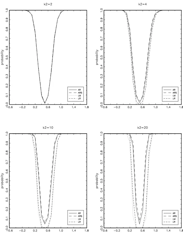
(26) Hence when Π2 is of full rank and the eigenvalues of A are positive, the projection-based confidence set for w0 β may be interpreted as a Wald-type confidence interval based on the statistic (which is asymptotically pivotal): q 0˜ 0 T = (w β − w β)/ σ ˆ 2 (w0 A−1 w) . u. 6. Monte Carlo evaluation In this section, we study projection-based statistical inference through Monte Carlo simulations. We especially focus on the evaluation of the degree of conservatism of the projection-based confidence sets (CS) and we compare the confidence sets obtained on the basis of different statistics. These statistics are the Anderson-Rubin statistic (AR) given by (2.9), the asymptotic AR statistic (ARS) given by (2.9) but without assumption (2.6) (it follows asymptotically a χ2 (k2 )/k2 distribution) and the LR and LM statistics proposed by Wang and Zivot (1998) and given by (2.13) - (2.14). We also study the behavior of the Wald statistic based on 2SLS. The data generating process is: y = Y1 β 1 + Y2 β 2 + X1 γ + u ,. (6.1). (Y1 , Y2 ) = X2 Π2 + X1 Π1 + (V1 , V2 ) ,   1 .8 .8 i.i.d. (ut , V1t , V2t )0 ∼ N (0, Σ) , Σ =  .8 1 .3  , .8 .3 1. (6.2) (6.3). with k1 = 1, G = 2, β 1 = 21 , β 2 = 1 , γ = 2 , and Π1 = (0.1, 0.2) . The correlation coefficient r between u and Vi (i = 1, 2) is set equal to 0.8, the variables Y1 and Y2 are endogenous and the √ instrumental variables X2 are necessary. The matrix Π2 is such that Π2 = C/ T . We consider three different sample sizes T = 50, 100, 200. The number of instruments (k2 ) varies from 2 to 40. All simulations are based on 10000 replications. Table 2 presents the results for C = 0 (complete unidentification), Table 3 presents the results for a matrix C with components cij such that 1 < cij < 5 (weak identification), and Table 4 with cij such that 10 ≤ cij ≤ 20. The nominal confidence level for all tables is 95%. We begin with the behavior of the classical Wald statistic (Table 1), As expected from the results in Dufour (1997), its real coverage rate may reach 0 when the instruments are very poor. The only case where it behaves well is when identification holds and the number of instruments is small compared to the sample size. This shows how crucial is the need for alternative valid pivotal statistics. For the exact AR statistic, no size distortion, even very small, is observed. The main observation is that the coverage rate of the projection-based confidence sets for β 1 decreases as k2 increases and tends to the exact confidence level 1 − α of the confidence set for β. 5 Thus the projection-based confidence sets become less conservative as the number of relevant instruments increases. This 5. Recall that theoretically, this rate is always greater than or equal to the confidence level of the set from which the projection is done.. 20.