Vincent: HEC Montréal, 3000 Chemin de la Côte-Sainte-Catherine, Montréal, QC, Canada. Tel. : +1 514 340 6419; fax : +1 514 340 6469; and CIRPÉE, Canada
Cahier de recherche/Working Paper 12-30
Price Stickiness in Customer Markets with Reference Prices
Nicolas Vincent
Abstract:
Price rigidity is often modeled by assuming that firms face a fixed cost of price change. However, in surveys, firms report that the main reason they wish to keep prices stable is for fear of antagonizing customers. Moreover, marketing studies show that most consumers engage in very little product comparison on a typical shopping trip. In this paper, we explore the implications of these observations for price rigidity. In our model, comparing prices and characteristics of alternative brands is time-consuming. While some consumers behave as bargain hunters with zero opportunity cost form shopping, most are loyal to firms as long as posted prices are not raised. A price increase is interpreted as a signal that a better alternative may be available and triggers consumer search. Firms do not face menu costs and are free to change nominal prices, but understand that their pricing decisions will affect their customer base and hence future profits. We show that this micro-founded mechanism is akin to a nominal rigidity and naturally generates price stickiness. It is also compatible with the observation of frequent sales at the retail level and can rationalize the decreasing or flat hazard functions observed empirically.
Keywords: Price stickiness, customer relations, nominal rigidities, consumer inattention
1
Introduction
Standard macroeconomic models require nominal rigidities to generate real e¤ects from monetary shocks. In addition, the degree of price rigidity has …rst-order conse-quences on the dynamic properties of such models. While a large body of research has evolved on the topic of price rigidity, both empirically and theoretically, a consensus on the main factors behind the observed stability of prices in micro data remains elusive.
In the context of macroeconomic models, attempts at generating price stickiness in the face of shocks have generally taken one of three forms. Originally and still up to this day, nominal rigidities have been modelled as reduced-form mechanisms such as Calvo pricing, also called time-dependent mechanisms. Here, the probability that a given …rm is allowed to reset prices is exogenous and outside of its control. While this mechanism has had some success for aggregate analysis, it is not based on micro foundations and cannot explain some of the micro stylized facts present in the data (see Bils and Klenow, 2004, and Nakamura and Steinsson, 2008).
Structural attempts at modeling this type of friction have mostly taken the form of menu costs. Under this state-dependent mechanism, the …rm faces a …xed cost to changing its nominal price and optimally chooses the moment of doing so. The modelling device naturally gives rise to sticky prices, i.e. periods during which prices remain unchanged. It does not however rationalize the presence of very frequent sales in the data, and requires additional assumptions in order to generate signi…cant real e¤ects from monetary shocks (see Golosov and Lucas, 2006, and Midrigan, 2011). More recently, models incorporating informational frictions on the side of …rms have been proposed in order to generate price rigidity (see Mankiw and Reis, 2002, as well as Mackowiak and Wiederholt, 2009).
Despite the fact that menu costs and costly information have been the two main micro-founded mechanisms used in macro models, based on survey evidence …rms in real life appear to give little weight to these two factors as reasons for keeping prices stable (see for example Blinder et al., 1998, and Fabiani et al., 2005). Instead, they emphasize concerns such as losing/angering customers or market share, considerations which have received very little attention in the price rigidity literature aside a few
exceptions. For example, Kleshchelski and Vincent (2009) embed customer switching costs in an otherwise standard macro framework. They show that the resulting cus-tomer base dynamics impact the pricing decision of the …rm and lead to more stable prices in the face of shocks. There are two limitations however. First, the mechanism leads to real instead of nominal rigidity. Second, unless it is paired with some menu cost, it does not generate prices which are sticky, i.e. that stay constant for prolonged periods of time. The current paper addresses these two issues.
Rotemberg (2005) uses a reduced-form speci…cation to model the concept of al-truism or fair pricing. In the model consumers see a …rm as "altruistic" if it does maximize a mixture of pro…ts and consumer utility. More speci…cally, consumers get signals about the …rm’s marginal cost. Using this information, they assess whether a price increase is "fair". If the consumer views the price as unfair, it stops buying the good. In other words, in the consumer’s mind, price increases which do not cor-respond to cost increases are likely to trigger anger and a large drop in sales. This gives rise to threshold e¤ects, insofar as consumers react very strongly (stop buying) as soon as the fairness condition is not met.
In more recent work, Rotemberg (2010) studies a framework akin to consumer regret. For example, a consumer who observes a price increase for a storable good may regret not having bought more of it in the past. Conversely, a price fall may trigger regret for not having waited to buy. This idea is modelled in a reduced form way by assuming that consumers incur a cost whenever a price is changed (the cost is a function of the size of the price change). In order for this feaure to a¤ect the pricing decision, the objective function is then altered to directly include a notion of altruism: the …rm maximizes a weighted function of its pro…ts and its customers’ utility. This naturally means that the "regret cost" (the cost of a price change for the consumer) is now internalized by the …rm. The result is something akin to a menu cost, which is always positive and increasing in the size of the price change. Hence, nominal price stickiness follows naturally. Arseneau and Chugh (2007) also explore the role of fairness issues in a search-based environment with bargaining and show that price rigidity can arise endogeneously, while Nakamura and Steinsson (2011) show that sticky prices can be an equilibrium in a setting with internal deep habits. The contribution of this paper is to o¤er a micro-founded mechanism which
gen-erates nominal price rigidity and rationalizes …rms’ revealed concerns about price changes potentially antagonizing customers, without relying on concepts of altruism or fairness. The otherwise standard macro model is based on a basic fact: comparing products, brands or even stores takes time and resources. It is particularly true of products which are purchased frequently. For example, consider a consumer who goes to the grocery store on a weekly basis to purchase a basket composed of multiple types of goods. In the event that he decides to actively shop for, say, toothpaste, he must compare brands and products across at least two dimensions, prices and char-acteristics (summarized by product-speci…c taste shocks in our speci…cation). Having chosen the option with the highest utility, he moves on to the next good. Clearly, active comparison shopping is not something he can realistically perform for most goods purchased on a given trip to the grocery store. On the next occasion, he must decide whether to take time to compare once again toothpaste brands, or instead to simply purchase his "home brand", i.e. the one he purchased in the past. In our model, positive shopping/search costs imply that the optimal consumer strategy is to use the nominal price of the home brand as a signal. If it rose since the price originally paid (the "reference price"), the customer scans the shelves to see whether a better alternative exists. If the price did not increase, he instead remains loyal to the brand. This is because absent any new information regarding the evolution of the distribution of product prices and characteristics, the consumer continues to believe that the brand he originally chose remains his best choice. And updating beliefs about the distribution would in turn require actively comparing products, a costly action.
We show that modifying the consumer problem along the lines just described generates signi…cant nominal price stickiness even in the case of economy-wide shocks. That is, even if all its competitors have been hit by a similar positive shock, a …rm is reluctant to raise its nominal price by fear of triggering search from its loyal customers. Not only are prices sticky, but the framework is in line with some well documented features of the data. First, unlike menu cost models, it is compatible with the presence of frequent temporary sales. A price fall will not lead loyal customers to react in our model: they will only see the sale price as a "bonus", making their home brand even more attractive. Second, our mechanism rationalizes the declining or ‡at hazard
functions observed in micro price data. As the …rm maintains prices constant, it attracts new customers and retains its loyal clientele. Consequently, its customer base grows larger, making a price increase ever costlier and hence less likely, until the markup has become too small to bear. Third, the mechanism gives rise to the well documented “rockets and feathers”phenomenon: prices rise faster following positive cost shocks than they fall as costs go down (see Peltzman, 2000, for evidence from multiple markets).
Our framework is related to the large literature in marketing on the concept of “reference price”, i.e the price to which consumers consciously or unconsciously com-pare the current observed store price. There is evidence that customers carry around an internal reference price: instead of re-optimizing at each shopping trip for every product by comparing brand prices, consumers tend to remember the last nominal price paid (reference price) and then compare it to the current price (see for example Kalyanaram and Little, 1994, Briesch et al., 1997, and Mazumbar et al., 2005). In line with our model, researchers in this …eld have identi…ed the opportunity cost of constantly re-optimizing as a factor behind this empirical …nding. Also, the fact that rising prices triggers search has been documented by Lewis (2011) in the gasoline market: he …nds that tra¢ c on the price comparison website www.gasbuddy.com is signi…cantly higher in periods when gas prices are on the rise.
The outline of the paper is as follows. Section 2 describe the economic environment as well as the maximization problems faced by households and …rms. In Section 3 we analyze the optimal pricing decision of the …rm in a partial equilibrium setting, while the mechanism is embedded within a general equilibrium framework in Section 4. Section 5 concludes.
2
Motivating evidence and literature
In order to explain the high degree of price rigidity present in the micro data (see Carlton, 1986, for early evidence, and more recently Bils and Klenow, 2005, or Naka-mura and Steinsson, 2009) economists have used a variety of mechanisms in their models. The two most common ways of modelling nominal price rigidity have been to implement time-dependent pricing a la Calvo, or assume the existence of menu
costs.
Table 1 reports some evidence from Fabiani et al. (2005). It gathers and sum-marizes the results from a number of price-setting surveys regarding the relative importance of various theories of price rigidity. The striking feature behind this ev-idence is the importance that …rms attach to factors linked to “customer relations”, despite the fact that the actual theory this category refers to may di¤er across sur-veys. For example, it includes the desire of sellers to maintain market share or a fear that changing prices may antagonize customers and disrupt long-term relationhips with the loyal clientele (see Okun, 1981). Blinder et al. (1998) observe that …rms often volunteer similar explanations when asked open-ended questions on price rigid-ity. While it might be di¢ cult to determine which of these variants is most relevant, our emphasis on factors related to customer base appears clearly in line with …rms’ actual concerns.
TABLE 1
Theories behind price rigidity
Euro US CA SW UK BE ES FR NL AT PT Customer relations 1 4 2 1 5 1 1 4 1 1 1 Menu costs 8 6 10 11 11 9 6 6 7 8 7 Costly information 9 - 10 13 - 8 7 - - 7 -# of theories 10 12 11 13 11 10 9 7 8 10 9
Note: Rank of di¤erent theories based on …rm surveys. Source: Fabiani et al. (2005)
Paradoxically, the two mechanisms which have probably garnered the most atten-tion in the state-dependent literature on price stickiness are considered less important by …rms. When managers are asked whether price rigidity might be the product of menu costs or costly information gathering, they invariably rank such theories very low.1 There is also evidence that the degree of price rigidity is related to customer
1One may rightly argue that menu costs could be interpreted more generally as inclusive of
customer-related costs. Yet in the way they are modelled in modern macroeconomic models, they would then represent a very crude reduced form. At a minimum, they would not take into account
base concerns. The survey on price-setting conducted in Canada by Amirault, Kwan and Wilkinson (2006) o¤ers evidence that there is a signi…cant correlation between the importance of customer relations and price stickiness. They report that “cus-tomer relations costs have a very high level of acknowledgement among …rms with the stickiest prices. Seventy-six per cent of …rms who change their prices only once or not at all during the year recognize this factor as a source of price rigidity”compared with 37% who adjust prices more than 52 times a year. This di¤erence is statistically signi…cant. Not surprisingly, …rms with a higher fraction of repeat customers are also those who are more concerned about factors linked to customer relations (see for ex-ample Apel, Friberg and Hallsten, 2005, or Hall, Walsh and Yates, 1997). In addition, there is evidence that …rms with a higher proportion of repeat customers tend to have more rigid prices. Aucremanne and Druant (2005) …nd that 43% of sticky-price …rms have more than 50% of repeat customers, versus 28% for ‡exible-price …rms.
Laboratory studies have also found evidence that price rigidity is more pronounced in the customer market than in an anonymous market. Cason and Friedman (2002) report that in their experiment, when sellers and buyers enter long-term relationships (here because customers face some costs of switching supplier), sellers will often absorb a portion of their cost changes in order to preserve their customer base. Similarly, Renner and Tyran (2004) …nd that “many sellers do not respond to the cost shock by increasing prices [...] because they hope to reap the gains from trading with loyal customers in the remaining periods of the game.”
While macroeconomists have paid little attention to the interaction between cus-tomer base and pricing, it is at the center of a large literature in marketing. In our model, the price previously paid becomes a reference price against which the currently posted price is compared. An important empirical literature in marketing has looked at the role of reference-price e¤ects in consumer decisions. Most applications have used past prices as a proxy for the reference price (see for example Lattin and Bucklin 1989, Hardie et al. 1993, or Kalyanaram and Little 1994) and have found that such models yield signi…cant improvements in …t. In addition, testing for the predictions of Kahneman and Tversky’s (1979, 1991) prospect theory, numerous studies have the dynamic dimension of customer base (i.e. long term impact of losing customers), an aspect which is at the heart of …rms’answers in surveys.
documented an asymmetric response of sales to price cuts and price increases (e.g. Briesch et al., 2000), sometimes also called “sticker shock e¤ect”.
Marketing research has almost exclusively looked into the relationship between reference price and brand choice. Yet, at its core, our mechanism is one where devia-tions of a price from its reference point is linked to search activity, which may or may not ultimately lead to brand switching. Yuan and Han (2011) show using market experiments that participants are more likely to search following price increases than decreases. In turn, this makes it optimal for sellers to raise prices drastically when they do so, but only slowly reduce prices in order to limit consumer search, a dynamic akin to the “rockets and feathers” phenomenon found in many markets (Peltzman, 2000). This result in a controlled environment is in line with the …ndings of Lewis (2009) in the gasoline market. He shows that tra¢ c on www.gasbuddy.com, a price comparison website, is signi…cantly higher in periods when gas prices are on the rise. Finally, it is also important to note that a number of well-documented pricing strategies by …rms are compatible with this type of mechanism. For example, pro-ducers and retailers often announce pre-emptively price hikes and provide the reasons behind the move, such as blaming the rise in the price of cotton for an increase in the prices of apparel. By appealing to aggregate forces to explain its action, a …rm may hope that consumers will interpret this situation as not …rm-speci…c, hence min-imizing the risk of customers switching brand or store. This would be consistent with the evidence from Gagnon (2009) who shows that in Mexico, a VAT increase led to a fast and widespread adjustment of prices across the economy. Also, limited attention by consumers rationalizes the frequent strategy of keeping prices constant while decreasing package size, as well as the heavy use of advertising alongside price drops.
3
The model
The economy is composed of a continuum of sectors/categories, each producing a product indexed by i 2 [0; 1]. In each sector, there is an in…nite number of …rms, each selling a distinct brand k 2 [0; 1]. Next we describe the optimization problems of the households and …rms.
3.1
Households
Each household derives disutility from labor L and utility from a basket of products C, and solves the following problem:
max U0j = E0 1 X t=0 tu (C t; Lt) u (Ct; Lt) = (Ct) 1 1 (Lt) 1+ 1 + subject to PtCt+ E0rt+1bt+1 = bt+ wtLt+ t
where E is the expectation operator and is the inverse of the elasticity of intertem-poral substitution, or risk aversion parameter. The household supplies homogenous labor and earns the economy-wide nominal wage rate wt. Households also have access
to complete state-contingent claims markets. The stochastic discount factor is given by rt+1 such that Etrt+1bjt+1 is the price at time 0 of a random payment b
j
t+1 in period
t + 1(we also impose a no-Ponzi-game constraint). Each household receives an equal share of the period t pro…ts from the …rms, t.
For expositional purposes and because the labor decision is standard, we focus in this section on the consumption problem of a representative household. In each period the consumer derives ‡ow utility from a basket of products according to a Dixit-Stiglitz aggregator, Ct= Z 1 0 c 1 j;t dj 1
where j denotes a category (e.g. sliced bread, cereal, orange juice, etc.) and is the elasticity of substitution across categories. This implies that the budget constraint can also be written as
Z 1 0
Within each category j there exists a continuum of brands which are valued by each consumer according to
cj;t =
Z 1 0
( k;j;t) 1 ck;j;tdk
where ck;j;t corresponds to the quantity consumed of brand k in category j in period
t. The consumer values brands di¤erently based on taste shocks drawn from a time-invariant distribution with cdf F . The exponent on the taste shock is inconse-quential and included only to ease exposition later on. Taste shocks here represent heterogenous preferences across consumers along various product characteristics (e.g. fat content, texture, presence of bleach). This setup implies that di¤erent products within a category are perfect substitutes (in the sense of having an elasticity of sub-stitution equal to in…nity), but have di¤erent valuations k;j;t. In this context, and
absent any constraint to brand switching, it is optimal for the consumer to choose every period the brand with the highest taste-to-price ratio.
From the household’s problem, the optimality conditions with respect to Lt and
bt+1 are standard. The …rst-order condition with respect to product j (assuming it
chose brand ) yields:
(Ct)
1
;j;t(c ;j;t)
1
= tp ;j;t (3.1)
where t is the multiplier on the household’s budget constraint and pj;t is the price
of the chosen brand k. Hence the household’s demand is zero for all brands except the one with the highest taste-to-price ratio:
c ;j;t=
p ;j;t ;j;tPt
Ct
The price index Pt as well as the aggregate basket Ct are household speci…c since
households potentially face di¤erent prices and taste shocks. However, in the sym-metric equilibrium, this will no longer be the case. Also, once we move to the problem of the …rm, we will drop the taste shocks from the demand schedules for expositonal purposes. They are irrelevant for pricing dynamics in our case since symmetry across brands implies that the composition of consumers (and their demand levels) will be
similar across …rms.
3.1.1 Search framework
As we already mentioned, if the consumer did not face any search cost, he would every period compare all brands within each category j and choose the brand with the highest taste/price ratio k;j;t=pk;j;t. In reality, however, search or shopping costs
are arguably non-negligible: for example, given the array of choices available for each product category in a typical grocery store, consumers cannot realistically spend time comparing all brands on a weekly basis.
For these reasons, we introduce in our model a positive shopping cost, s. That is, in a given period there is a time/…xed cost associated with learning about the price distribution and then comparing personal preferences across brands within a category. As long as the consumer purchases the same brand he purchased in the previous period, this cost is avoided. As an example, consider a shopper who is approaching the toothpaste aisle at the supermarket. The consumer locates the brand he usually buys and sees its price. He then needs to decide whether to simply purchase the same brand again, or start comparing all brands on display along both the price and taste dimensions.2
For tractability reasons we model the search cost as reducing directly the utility contribution of the category in question. Hence, letting hj;t = 1 if search is happening
in category j at time t, the consumption aggregate can be expressed as:
Ct= Z 1 0 (1 s)hj;t c 1 j;t dj 1
We now turn formally to the decision of a household to engage in active comparison shopping for an isolated product category . If the consumer decides not to search, he simply continues to enjoy the utility attached to the brand previously bought. Formally, the value at time t of not engaging in comparison shopping for category is given by
Wns;t = u (Ct; Lt; h;t = 0)
2One would expect heterogeneity across households in terms of search costs. In the full version
where time-t ‡ow utility was de…ned earlier. Alternatively, if the consumer decides to incur the shopping cost s, he sees the entire continuum of brand prices, pk; ;t,
and draws brand-speci…c taste shocks, k; ;t. By the law of large numbers, the entire
distribution of taste shocks is realized. Hence, the expected value of doing comparison shopping is given by
Wts= Etu (Ct; Lt; h;t = 1)
The consumer will decide to search if: Wts> Wtns
Notice that since we study the decision to search for category j in isolation, the only uncertainty that matters is the one related to the utility the consumer expects to obtain if it were to incur the search cost and engage in active shopping in category . Given the speci…cation of our utility function, the decision rule therefore boils down to a simple comparison at the category level:3
Et (1 s) c 1 ;t > c 1 ;t Et 2 4(1 s) pk; ;t k; ;tPt Ct ! 13 5 > ( ; ;t) p ; ;t Pt Ct ! 1 (1 s) Et " k; ;t pk; ;t 1# > ; ;t p ; ;t 1
Notice that because of our directed search setting, the expected utility from shop-ping is actually determined by the maximal taste-to-price ratio the consumer after comparing price and product characteristics. Hence, for a small enough search cost s, the consumer will decide to shop if he expects to …nd a brand with a higher taste-to-price ratio than the one he is currently consuming. But when it was initially chosen periods ago, the current brand itself represented the highest taste-to-price ratio available.
3To see this, one simply needs to write down the full expression for the ‡ow utility at time t and
Therefore, it is optimal for the consumer to remain loyal to the brand he has been purchasing as long as the price p ; ;t is not increased above the "reference price"
p ; ;t , that is the price at which the consumer originally purchased the product in
period t . Indeed, if p ; ;tis lower or equal than the consumer’s reference price, then
based on his beliefs about the price distribution the "next best brand" is now even less interesting in relative terms. Hence, as long as the price does not rise, the consumer will continue purchasing the same brand unless there is exogenous separation or if he gets exogeneous information regarding changes in the price distribution.
However, if p ;j;t does increase above the reference price p ; ;t , barring any new
information regarding the price distribution over the previous periods the consumer now believes by continuity that there exists a brand out there which is at least slightly better in the taste/price ratio dimension. Given a search cost small enough, he has an incentive to shop, learn the time-t price distribution, compare products and potentially switch brand.4
3.1.2 Discussion
Given our primary interest in price rigidity, so far we have focused on the optimal response of a customer to movements in the price of his home brand. Before moving on to the pricing decision of the …rm, we highlight a number of other potentially interesting implications of our reference price setting.
First, consider a category-wide positive cost shock. In our environment, an indi-vidual …rm raising its price would have an incentive to communicate to its customers that the shock is common to all …rms in the sector. By doing so, it will change the beliefs of consumers about the price distribution and minimize the search response of its customer base.
Second, because the reference point is de…ned along the price dimension, …rms may
4We are making the implicit assumption that the consumer picks the brand with the highest
taste-to-price ratio based on today’s prices only. Yet, with positive search costs, expectations about future prices for each brand should enter the decision process. This is, unfortunately, a very complex problem to solve. One realistic way to rationalize our modelling assumption would be to introduce some …xed cost of computing expectations about future prices for all available brands. Also, this issue is unlikely to be of signi…cant importance in our setup since shopping costs will be assumed to be very small. A …rm therefore has very limited ability to raise prices in the future to take advantage of locked-in loyal customers.
have an incentive to change product attributes instead of prices. Take the example of a 15 oz. cereal box with a posted price of $3, or 20 cents per ounce. In our framework, a consumer is more likely to react to an increase in the price to $3.75 than a change in package size to 12 oz., even though the price-per-pound increase in both cases is the same.
Third, the presence of temporary price cuts (“sales”) does not trigger search in our model: the customer only sees the price cut as a bonus which makes the brand even more interesting than before. Hence, as we will discuss later, our mechanism is compatible with the observation of frequent temporary sales in the data.
Fourth, limited attention by consumers implies a potentially strong role for ad-vertising by …rms in order to shape consumers’beliefs about the price distribution.
3.2
Firms
A brand k in category j is produced by a single-product …rm. In each category there are two types of …rms denoted by A and B, with a continuum of brands of each type. All …rms of a given type are identical and share the same technology (marginal cost). Hence they will all be charging the same price and, by the law of large numbers applied to taste parameters, have the same customer base in equilibrium.
In order to focus on the important elements of the framework, we present the canonical form of the model and postpone discussion of additional elements to future sections. The basic problem of the …rm in its recursive …rm is given by
max
pt
Vt= (pt ct) qt+ EtVt+1
where pt, ct, and qtare the price, marginal cost and quantity sold at time t respectively.
To simplify the exposition we leave aside for now the production dimension and do not include the brand/type/category subscripts.
In line with the consumer setup described in the previous section, a pro…t-maximizing …rm needs to keep track of vintages of consumers indexed by when they …rst purchased the …rm’s brand. This information is central to determining what will be the impact of the pricing decision on the …rm’s customer base. Leaving aside brand/category sub-scripts for clarity purposes, denote by m the mass of customers of vintage , those
who …rst bought from the …rm periods ago at price pt (the "reference price" from
the point of view of these consumers). If we denote by ut the number of units bought
by each consumer, then the total quantity sold by the …rm is equal to
qt= ut m0t + X =1 I (pt pt ) mt ! (3.2)
This expression follows from the consumer problem described earlier. As an ex-ample consider the case of = 1. Here m1
t corresponds to the mass of customers who
…rst bought the …rm’s brand the previous period, at price pt 1. If period-t price is
lower or equal than pt 1, these customers will remain loyal and continue to purchase
the same brand: having already chosen the best taste/price ratio during their com-parison shopping last period, the current price cannot make them worse o¤ and it is therefore optimal for them not to incur the positive shopping cost. Alternatively, if pt > pt 1, by continuity consumers know that there exists a better brand out there.
With a low enough shopping cost s, they decide to compare brands according to the framework described in the previous section. The same logic applies to older vintages = 2; 3; ::: Note that the mechanism is linked to nominal price levels, not relative prices. This is due to consumers not updating beliefs about the price distribution unless they pay the shopping cost and actually take the time required to compare competing brands.
The variable m0
t has been isolated in expression (3.2) because it does not refer
to loyal customers but instead new arrivals. Denote by St the mass of unattached
shoppers in the economy: they are consumers who decided to do comparison shopping following price hikes. Based on the price charged by the …rm (pt) and the distribution
of prices in the category (Fpt), a fraction f (pt; Fpt) of St will pick the brand in
max pt Vt= (pt ct) ut m0t + X =1 I (pt pt ) mt ! + EtVt+1 subject to m0t = Stf (pt; Fpt) mt+1+1 = I (pt pt ) mt
where the last line represents the law of motion of the customer base.
In the next section we study the …rm’s optimal pricing decision under this setup. In particular, we show that price stickiness is an equilibrium outcome of our model.
4
Price stickiness with reference prices
4.1
A numerical example using the basic framework
We …rst solve numerically the problem of a typical …rm and show simulations for the optimal price path in the wake of an idiosyncratic shock, holding the aggregate and sectoral state variables constant. Then, we look at the nominal nature of our friction by analyzing the response to a shock that would a¤ect all nominal variables proportionately in our economy. In addition, we discuss why the presence of sales is compatible with our mechanism. Finally, the basic model is enhanced in order to study more speci…cally the role of customer base dynamics, and trend in‡ation is introduced.
First, we simplify the general version of the model to minimize the number of state variables. To do so, we assume that loyal customers draw a zero shopping cost (s = 0) every other period, at which point they automatically shop across brands.
Consequently, the …rm needs only to keep track of a single vintage of loyal customers: max p V c; p 1; m 1 = (p c) u m0+ I (p p 1) m1 + EV c0; p; m1 0 ; subject to m0 = Sf (p; Fp) m10 = m0 c0 2 fc0; c1; c2g
where the variables have been described earlier. For the current analysis we treat c, S and Fp as …xed parameters, and the per consumer demand function is of the CES
type: u = (p=P ) , where P is a price aggregate and is the elasticity of substitution across categories. Also in this particular case it is clearer if we de…ne a new variable Awhich corresponds to the mass of new consumer arrivals, i.e. A = m0 = Sf (p; F
p).
For the numerical exercise of this section, Fp corresponds to a normal distribution of
mean pcomp and standard deviation comp. The …rm’s problem can then be expressed
as: max p V (c; p 1; A 1) = (p c) [A + I (p p 1) A 1] u + EV (c 0; p; A) subject to A = Sf (p; Fp) u = (p=P )
Because of the non-convexity in the objective function around p 1, it is not
pos-sible to use perturbation methods. Instead, we solve this model using value function iteration by de…ning grids for the marginal cost c, the previous price p 1and the choice
variable p. Notice that in the version above, the state variable A 1 is redundant as
it is completely determined by p 1.
Figure 4.1 below shows a sample price path simulated using the model. For this particular example, the parameter values are pcomp = P = 1:083, comp = 0:1, = 0:5,
= 5; and the marginal cost c follows a 5-point Markov chain with mean 1, standard deviation 0:02 and serial correlation 0:8. The blue line represents the marginal cost
500 520 540 560 580 600 620 640 660 680 700 0.94 0.96 0.98 1 1.02 1.04 1.06 1.08 1.1 1.12 1.14
Figure 4.1: Response of prices (green) to marginal cost shocks (blue). while the green line is the evolution of the price series pt.
we bring attention to some of implications of our model. First, the price series in less volatile than marginal costs. Second, the model generates naturally price sticki-ness: the price series exhibits clear periods of inaction despite underlying changes in the marginal cost. This implies that the markup, p c, exhibits signi…cant variations. Third, price dynamics display something akin to the "rocket and feathers" pattern documented in the literature (see Peltzman, 2000, for evidence of such pattern in a large number of producer and consumer goods): at a certain point, when the markup becomes too small, the price eventually shoots up rapidly. Then, as the marginal cost goes back down, prices also fall but more slowly.
To understand the intuition behind these results, consider the following example: starting from an equilibrium situation where all …rms charge the same price, one brand is hit at time t by an increase in its marginal cost. We analyze whether there is an incentive for a particular …rm to deviate and raise its price. For expositional purposes we assume that the shopping cost s is epsilon small.
If the …rm raises its price, it is able to maintain at least partially its initial markup level. However, the price increase has a negative impact on quantity: along the
extensive margin, this decision will lead all loyal customers who have a reference price equal or lower than pt to compare brands. This set of "leavers" is not empty,
since consumers who bought from the …rm for the …rst time at t 1at reference price pt 1 will …nd it optimal to pay the shopping cost, draw a new distribution of taste
shocks and look for the brand with the highest taste/price ratio. Of these unattached shoppers, less than the usual number will choose the …rm again since its price is now higher. In addition, the rise in price will have a negative impact on the quantity sold per consumer.
If the …rm decides instead to keep its price constant it will retain its entire customer base, at the expense of facing a lower markup. When the marginal cost increase is not too large, price stickiness is the optimal pricing strategy: the seller accepts lower pro…t margin in order to avoid losing a positive mass of customers to the competition. Also, a price fall is a dominated strategy in this setting, as …rms could have implemented it the previous period before the marginal cost increase.
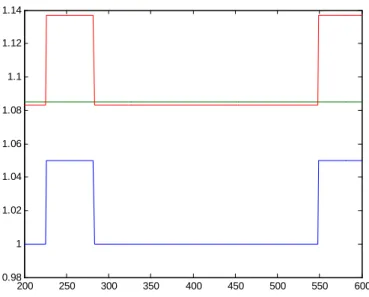
The previous exercise shows that the mechanism proposed can generate signi…cant relative price stickiness, i.e. the …rm may decide to keep its price constant when it is the only one hit by the shock. To determine whether it also generates nominal price rigidity, one needs to analyze the …rm’s optimal price decision following a common shock. We make a simple extension to the current model. The economy now alternates between two very persistent aggregate states: in the high state, all nominal variables (the marginal cost c, the mean of the price distribution of competing brands pcomp,
as well as the aggregate price level P ) are multiplied by a common factor ! > 1. In order to focus on the impact of this pseudo-aggregate shock, the variance of the idiosyncratic marginal cost is set to 0.
Figure 4.2 depicts the simulated values for the …rm’s price (green), the marginal cost (blue) as well as the average price of the competing brands pcomp(red) in an
environment where ! 2 f1; 1:05g. Notice that even if all other brands were to raise their prices by 5%, in line with the marginal cost increase, the …rm would have no incentive to deviate from its current price. In other words, what is costly for the …rm is to lift its nominal price. This is because the margin that triggers search is the di¤erence between the posted price and the reference price of the consumer, not the relative posted price across brands in the current period. Eventually, with a larger
200 250 300 350 400 450 500 550 600 0.98 1 1.02 1.04 1.06 1.08 1.1 1.12 1.14
Figure 4.2: Nominal price stickiness in response to aggregate shocks. Retailer price (green), competitors’prices (red) and marginal cost (blue).
aggregate shock, the …rm would …nd it optimal to adjust its price to a new level. One interesting implication of this …nding is that …rms have an incentive to com-municate credibly to their customers that the shock is common to all brands. This is because by doing so, the announcement will shift the consumers’beliefs about the entire distribution of competing brands. Hence, if the customer believes that all prices have gone up by x%, he will have no incentive to search.
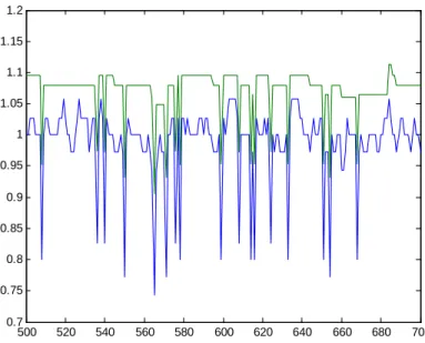
Next, we implement a role for sales. We think of a sale coming from a fall in the marginal cost, in line with Kehoe and Midrigan (2010) and scanner data studies (see examples from Rotemberg, 2005, or Eichenbaum, Jaimovich and Rebelo, 2011). In other words, at this point we do not try to model the reason why the supplier implements these sales in the …rst place. Here, a sale is extremely temporary (1 period), and retrieves 0.2 from the value of the current regular marginal cost. Figure 4.3 shows an example of a simulated price series:
This pattern for the price and marginal cost is very reminiscent of what can be seen in the scanner data. Notice that even though …rms are very reluctant to raise prices, they have no problem passing through a signi…cant portion of the large fall in
500 520 540 560 580 600 620 640 660 680 700 0.7 0.75 0.8 0.85 0.9 0.95 1 1.05 1.1 1.15 1.2
Figure 4.3: Sales in the baseline model. Price (green) and marginal cost (blue). marginal cost. This is because loyal customers see this sale price as a bonus, and are not inclined to search once the price goes back to its regular level.
4.2
A modi…ed model with richer dynamics
The model of the previous section, while very clean, displays limited dynamics: since consumers draw a zero search cost every other period, there is not much of a concept of building a loyal customer base. In fact, in the simple version used for the numerical exercise, the number of loyal customers that have been retained at time t will anyway leave at time t + 1. One option is to increase the number of overlapping customer vintages, but this would raise substantially the computational burden as it would be necessary to keep track of the state variables m and pt . Instead, we make the
model richer and more dynamic by implementing three simple modi…cations to the basic framework.
First, in every period a fraction of loyal customers is hit by an exogenous shock (e.g. zero search cost, advertising) that leads them to search and compare brands, whether there has been a price increase or not. Second, in the event of a price increase,
a fraction of loyal customers shop and learn about the price distribution but decide to stay with their home seller anyway. It could be for example because they realize that their switching cost is too high. They will remain part of the customer base until at least the following period. Finally, loyal customers draw a zero search cost after two periods. Of them, a fraction decide that they want to remain attached to their home brand. More precisely, we assume that their taste shock (or some exogenous switching cost) is such that the home brand remains the one with the highest taste-to-price ratio.
In this context, it is necessary to keep track of the size of the …rm’s customer base and the optimization problem in recursive form becomes:
max p V (c; p 1; L) = (p c) [A + I (p p 1) (1 )L + I (p > p 1) (1 )L] u + EV (c 0; p; L0) subject to A = Sf (p; Fp) L0 = A + I (p p 1) (1 ) L + I (p > p 1) (1 ) L
Once again the problem is solved using value function iteration, with an additional grid for the new state variable L. Any decision p, coupled with the initial state (p 1; L), determines a unique customer base next period of L0. We simulate the
model with the following parameter values: S = 1, = 5, = 0:5, = 0:1; = 0:8; = 0:5. The price distribution Fpb is time invariant with mean of pcomp = 1:1
and standard deviation 0:1. The marginal cost follows a 5-point Markov chain with standard deviation 0:025 and serial correlation 0:8.
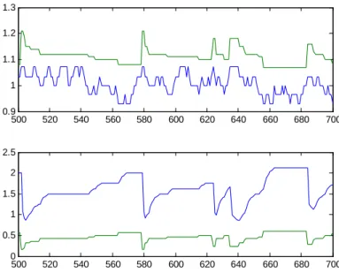
The top plot of Figure 4.4 shows the marginal cost (blue) and price (green) series over 200 periods. The price change frequency is equal to 11:3% versus 45:8% for the marginal cost series. In other words, prices are sticky as not all marginal cost changes translate into price movements (see Eichenbaum, Jaimovich and Rebelo, 2011, for supporting evidence). As seen earlier, the …rm resists raising prices until the markup is too small to bear, at which point the price is adjusted upward suddenly. Subsequent downward movements in the marginal cost are met with smaller price decreases up to a new sticky price level. The bottom plot shows the evolution of the customer base L
500 520 540 560 580 600 620 640 660 680 700 0.9 1 1.1 1.2 1.3 500 520 540 560 580 600 620 640 660 680 700 0 0.5 1 1.5 2 2.5
Figure 4.4: Dynamic model. Top panel: price (green) and marginal cost (blue). Bottom panel: new arrivals (green) and customer base (blue)
(blue) and the mass of new arrivals A (green). Price increases lead to signi…cant drops in both the customer base and new arrivals. This should not be surprising: when the price is raised it tends to be by a signi…cant amount (the median price increase is 10% in this example). We can also see the customer base dynamics at play: after raising its price, the …rm attracts some new customers and slowly rebuilds its customer base, to a lower level if the new price stabilizes to a higher level than the old price.
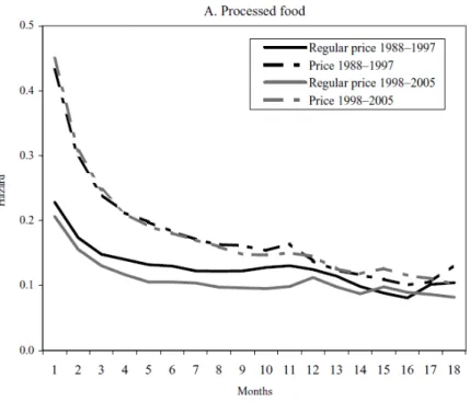
We now turn to the hazard function generated by our model. The hazard rate for a given point t shows the probability that a price is changed after exactly t periods. A basic Calvo model predicts that the hazard function is ‡at (the probability of a price change is not a function of how long since the last price reset), while a menu cost model generally predicts an upward sloping pattern (a price that has been kept constant for a long period is more likely to be changed). Empirically, Nakamura and Steinsson (2008) show that using CPI data, the hazard function initially declines sharply become somewhat ‡attening out (we reproduce their …gure for processed food below). Based on their simulations, they con…rm that a simple menu cost model does not appear to be able to match this type of pattern.
Figure 4.5: Hazard functions from Nakamura and Steinsson (2009)
In Figure 4.6 we plot the hazard function for the parameterization described above. The sharp decline in the hazard function in the …rst few periods comes from the fact that following a price increase, a retreat of the marginal cost will lead to gradual declines in the price charged. This comes directly from the fact that the marginal cost process does not include any trend in‡ation, an assumption that we relax later on. Beyond this initial sharp decline, there is another force at play: as the …rm refrains from increasing its price, it slowly builds up its customer base. But as loyal customers become more and more prominent versus new arrivals every period, it also implies that any price increase becomes relatively more costly. Therefore, the longer the …rm waits to raise its price, the less likely it is to do so in the future, all else being equal. Also, it should be noted that in this version of the model with dynamic customer base, a price change can occur at time t even though there has been no movement in the marginal cost during this period. This stems from the role of the customer base L as a state variable.
0 10 20 30 40 50 60 70 80 90 100 0.02 0.04 0.06 0.08 0.1 0.12 0.14 0.16 0.18 0.2 0.22
Figure 4.6: Hazard function from the model
4.3
Introducing trend in‡ation
We now introduce trend in‡ation. Our framework is an adaptation of the simple partial-equilibrium menu cost model from Nakamura and Steinsson (2008). The pro-duction function of the …rm is given by
yt = ztLt
where the …rm-speci…c productivity level has the following law of motion log (zt) = log (zt 1) + "t
The real wage rate is constant at Wt=Pt = w: The aggregate price level is
exoge-nous and ‡uctuates around a trend
log Pt+1= + log Pt+ t
aggregate price level P every period, and that the variance of the within-category price distribution is time-invariant. The …rm knows P and z before choosing p.
We can write the real pro…t function for a given period as
= p P w A " A + I (p p 1) (1 )L + I (p > p 1) (1 )L # p P
and the …rm’s intertemporal problem expressed in real terms is
max p V z; p 1 P ; L = p P w z " A + I (p p 1) (1 )L + I (p > p 1) (1 )L # p P + EV c 0; p P0; z 0 subject to A = Sf p P; Fp L0 = A + I (p p 1) (1 ) L + I (p > p 1) (1 ) L log (z) = log (z 1) + " log P0 = + log P +
To solve this problem by value function iteration, we need to de…ne grids for the three state variables. We approximate the dynamics of z and by using nz and n
-point Markov chains respectively (note that the uncertainty regarding P0 is resolved
in the current period). We de…ne the new variable ^p = log p 1
P which allows us to
rewrite the problem as:
max p V (z; ^p 1; L; ) = p +^ + 1 w z " A + I (^p 1 p^ ) (1 )L + I (^p 1 p < ) (1^ )L # (^p + + 1) + EV (c0; ^p0; z0; 0) subject to ^ p 1 = log p 1 P ; p = log^ p P0 A = Sf (^p + + 1; Fp) L0 = A + I (^p 1 p^ ) (1 ) L + I (^p 1 p < ) (1^ ) L
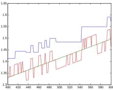
400 420 440 460 480 500 520 540 560 580 600 1.3 1.35 1.4 1.45 1.5 1.55 1.6 1.65
Figure 4.7: Introducing trend in‡ation. Firm price (blue), marginal cost (red) and aggregate price level (green).
and de…ne a linear grid for ^p (we need to make sure that the possible values of are on the support of the grid). Figure 4.7 shows the evolution of the optimal price, the aggregate price level as well as the nominal marginal cost in a simulation from our model. The …rm resets its price to bring back its markup to some average desired level, and there are extended periods of sticky prices at it does not respond to marginal cost movements.
5
Conclusion
In this paper we present a micro-founded mechanism which generates nominal price rigidity and rationalizes …rms’revealed concerns about price changes potentially an-tagonizing customers, without relying on concepts of altruism or fairness. The friction stems from a basic fact: comparing products, brands or even stores takes time and re-sources. In our model, consumers engage in price comparison only when they believe doing so may lead them to a better brand. We show that modifying the consumer problem along these lines generates signi…cant nominal price stickiness even in the
case of economy-wide shocks. That is, even if all its competitors have been hit by a similar positive shock, a …rm is reluctant to raise its nominal price by fear of trigger-ing search among its loyal customers. Not only are prices sticky, but we also argue that the predictions of the framework are in line with some well documented features of the data. In addition, the mechanism rationalizes …rm strategies that appear puz-zling in the context of a standard model. For example, in our environment there is an incentive for the seller to publicize that a shock is common across brands in order to minimize search among its customers. Also, since consumer search is triggered by a change in the nominal price and other attributes are not observed on every shopping occasion, it can be rational for a …rm to keep prices constant but lower packaging size to avoid an adverse reaction by its customer base.
Future work will look at the general equilibrium implications of this mechanism. In addition, there are interesting extensions to be explored, such as the role of advertising in this setup, the strategy of adopting price points and the possibility of multiple equilibria.
References
Apel, M., R. Friberg and K. Hallsten, 2005. Microfoundations of Macroeconomic Price Adjustment: Survey Evidence from Swedish Firms. Journal of Money, Credit and Banking, Vol. 37, No. 2, 314-338.
Amirault, D., Kwan, C., and G. Wilkinson, 2006, “Survey of Price-Setting Behaviour of Canadian Companies”, Bank of Canada Working Paper 2006-35.
Arseneau, D. and S. Chugh, 2007. Bargaining, Fairness, and Price Rigidity in a DSGE Environment. mimeo University of Maryland.
Aucremanne, L. and M. Druant, 2005. Price-Setting Behaviour in Belgium: What Can Be Learned from an Ad-Hoc Survey?, ECB Working Paper No. 448.
Bils, M., Klenow, P., 2004. Some evidence on the importance of sticky prices. Journal of Political Economy, Vol. 112, No 5, 947-985.
Blinder, A.S., E.R.D. Canetti, D.E. Lebow and J.B. Rudd , 1998. Asking about Prices: A New Approach to Understanding Price Stickiness, New York: Russell Sage. Briesch, R. A., L. Krishnamurthi, T. Mazumdar, S. P. Raj, 1997. A comparative
analysis of reference price models. J. Consumer Res. 24 (September) 202-214. Carlton, Dennis W. 1986. The Rigidity of Prices. American Economic Review 76
(September): 637–658.
Eichenbaum, M., Jaimovich, N. and S. Rebelo, 2011. Reference prices and nominal rigidities. American Economic Review, 101(1), 234-62.
Fabiani, S., Druant, M., Hernando, I., Kwapil, C., Landau, B., Loupias, C., Martins, F., Matha, T.Y., Sabbatini, R., Stahl, H. and A.C.J. Stockman, 2005, “The Pricing Behaviour of Firms in the Euro Area”, ECB Working Paper No. 535. Gagnon, Etienne, 2009. Price Setting during Low and High In‡ation: Evidence from
Hardie, B. G. S., E. J. Johnson, P. S. Fader, 1993. Modeling loss aversion and reference dependence e¤ects on brand choice. Marketing Science, 12(4) 378–394.
Kahneman, D. and A. Tversky, 1979. Prospect Theory: An Analysis of Decision under Risk. Econometrica, 47(2). 263-291.
Kahneman, D. and A. Tversky, 1991. Loss Aversion in Riskless Choice: A Reference-Dependent Model. The Quarterly Journal of Economics. Econometrica, 106(4). 1039-1061.
Kalyanaram and Little,1994. An Empirical Analysis of Latitude of Price Acceptance in Consumer Package Goods. The Journal of Consumer Research, Vol.21, No.3 Kehoe, P. and V. Midrigan, 2010. Prices are Sticky After All, mimeo, New York
University.
Kleshchelski, I. and N. Vincent, 2009. Market Share and Price Rigidity. Journal of Monetary Economics, 56(3), 344-352.
Lattin, J. M. and R. E. Bucklin, 1989. Reference E¤ects of Price and Promotion on Brand Choice Behavior. Journal of Marketing Research, Vol. 26, No. 3 (Aug., 1989). 299-310.
Lewis, M. 2011. When Do Consumers Search? Journal of Industrial Economics, 93(2). 672-682.
Mackowiak, B. and M. Wiederholt, 2009.Optimal Sticky Prices under Rational Inat-tention. American Economic Review, 99(3), 769-803.
Mankiw, G. and R. Reis, 2002. Sticky Information Versus Sticky Prices: A Proposal to Replace the New Keynesian Phillips Curve. Quarterly Journal of Economics, 117(4). 1295-1328.
Midrigan, V., 2011. Menu Costs, Multi-Product Firms, and Aggregate Fluctuations. Econometrica, 79(4). 1139-1180.
Nakamura, E. and J. Steinsson, 2008. Five facts about prices: a reevaluation of menu cost models. Quarterly Journal of Economics, 123(4), 1415-1464.
Nakamura, E. and J. Steinsson, 2011. Price Setting in Forward-Looking Customer Markets. Journal of Monetary Economics, 58(3). 220-233.
Okun, A. ,1981. Prices and Quantities: A Macroeconomic Analysis, Blackwell:Oxford. Peltzman, S., 2000. Prices Rise Faster Than They Fall. Journal of Political Economy,
Vol. 108 (2000). 466–502.
Renner, E. and J.-R. Tyran, 2004. Price Rigidity in Customer Markets. Journal of Economic Behavior & Organization, Vol. 55, 575-593.
Rotemberg, J, 2005. Customer Anger at Price Increases, Changes in the Frequency of Price Adjustment and Monetary Policy. Journal of Monetary Economics 52(4). 829-852.
Rotemberg, J, 2010. Altruistic Dynamics Pricing with Customer Regret. Mimeo, Har-vard Business School.
Yuan, H. and S. Han, 2011. The E¤ects of Consumers’Price Expectations on Sellers’ Dynamic Pricing Strategies. Journal of Marketing Research, Volume 48, Number 1, February 2011.