A THREE-STEP PROCEDURE IN SAS TO ANALYZE THE TIME SERIES FROM AUTOMATIC DENDROMETERS
Annie Deslauriers*, Sergio Rossi, Audrey Turcotte, Hubert Morin and Cornélia Krause Département des Sciences Fondamentales, Université du Québec à Chicoutimi, 555 Boulevard de l'Université, Chicoutimi (QC), Canada G7H 2B1
5
ABSTRACT
Continuous measurements of stem radius variation in trees are obtained with automatic dendrometers that provide time series composed of seasonal tree growth and circadian 10
rhythms of water storage and depletion. Several variables can be extracted from the raw data, such as amplitude and duration of radius increase and contraction, which are useful for understanding intra-annual tree growth, tree physiology and for performing growth-climate relationships. These measurements constitute a large dataset whose manipulation needs numerous algorithms and automatic procedures to efficiently and rapidly extract 15
the information. This paper presents a three-step procedure using two SAS routines to extract the time series describing radius variation and associate them with environmental parameters. The first routine organizes and corrects data and generates outputs in the form of files and plots to visualize the results and improve data correction (first step). The second step consists of a reclassification of the hours of contraction or expansion that 20
have been misclassified by the automatic process. The second routine classifies the daily patterns of stem variation into the three phases of contraction, expansion and radius increment and associates the environmental parameters (third step). An example of the procedure is given, with an explanation of the outputs generated. The advantages and shortcomings of the procedure and its importance for the intra-annual analyses of tree 25
growth are discussed.
1. INTRODUCTION
In agronomy and forestry, automatic dendrometers are frequently used to continuously 30
record growth in organs such as fruits and stems. In forestry, they measure the radial variations of stem and roots, composed of diurnal rhythms of water storage depletion and replenishment (Kozlowski and Winget, 1964; Herzog et al., 1995; Offenthaler et al., 2001) and tree growth (Dünisch and Bauch, 1994; Tatarinov and Čermák, 1999; Tardif et al., 2001; Bouriaud et al., 2005). Detailed analyses of stem variation have recently been 35
obtained, providing daily patterns of radius variation, daily shrinkage and their duration. These parameters are becoming very useful for understanding the growth dynamics of trees (Deslauriers et al., 2007a; Giovannelli et al., 2007; Drew et al., 2008, 2009a; Turcotte et al., 2009). However, algorithms are necessary in order to efficiently manage the datasets and extract information from the raw data. The huge numbers of records 40
produced by measuring radius variation in continuum (after one year of hourly
measurements, a single dendrometer produces 8760 data points) obviously encourage the development of programs that automatically manage these data.
The extraction of stem radius variation throughout the year is the first step to obtain time series that can be used for studying intra-annual tree growth. In data analysis, two
45
approaches can be identified: (i) extracting one value per day (mean or max) from the time series (Tardif et al., 2001; Bouriaud et al., 2005), or (ii) considering the patterns of stem shrinking and swelling (Herzog et al., 1995; Downes et al., 1999). In the latter approach, the three distinct phases of contraction, expansion and stem radius increase are isolated and analyzed separately. The three phases approach is a reduction of the five 50
phases of the diurnal courses of the flow through the stem and the related changes in stem radius as defined by Herzog et al. (1995). The three phases approach was proposed by Downes et al. (1999) as it was computationally simpler that the five phases approach and therefore it is better suited for a signal processing application. Both approaches calculate very similar series of stem radius variation, although higher amplitude can be calculated 55
with the stem cycle approach as a cycle can last for more than one day (Deslauriers et al., 2007b). Specific parameters, such as stem shrinkage, hours and rates of stem increment (Deslauriers et al., 2007a; Drew et al., 2008), or other variables characterizing the cycles (Turcotte et al., 2009), can only be obtained with the stem cycle approach.
During the last years, intra-annual time series characterizing stem radius changes have 60
been used in a wide variety of studies. For instance, maximum daily shrinkage (MDS) is a suitable indicator of changes in plant water status and water stress (Conejero et al., 2007; Giovannelli et al., 2007; Ortuño et al., 2009). Stem radius increment (R) has been
more widely used as it represents an estimation of tree growth and correlates with physiological or environmental parameters. In a high-altitude environment in the Italian 65
Alps, R was directly linked with precipitation and sap flow during the night (Deslauriers
et al., 2007a). In eucalyptus trees, temperature was correlated with the rates of R
radius change include radial variation in wood properties (Wimmer et al., 2002; Bouriaud 70
et al., 2005; Drew et al., 2009b).
This paper presents a three-step procedure using SAS routines based on the stem cycle approach. The procedures include appropriate algorithms for the phase and cycle
divisions in order to extract the parameters describing stem radius variation and associate them with the meteorological variables. The stem cycle approach and the application 75
process will be described with an example. The most relevant analyses that can be obtained with these SAS routines and their importance in different fields are then outlined.
2. ANALYTICAL APPROACH
80
The stem cycle approach provides an accurate assessment of the components of the diurnal stem cycle: phase duration (hour) and stem radial variation, defined as stem radius increment (∆R, mm) and maximum daily shrinkage (MDS, mm) (Fig. 1). The extraction of these components is performed by dividing the stem cycle into three distinct phases (Downes et al., 1999 modified by Deslauriers et al., 2007a) as follows: contraction 85
(i), the period between the morning maximum and afternoon minimum; expansion (ii), the total period from the minimum to the next morning maximum; stem radius increment (iii), part of the expansion phase from the time when the stem radius exceeds the morning maximum until the subsequent maximum (Fig. 1).
The difference between the expansion maximum and the onset of stem radius increment 90
represents the positive stem radius increment (∆R+). When the previous cycle maximum is not reached, a negative stem radius increment (∆R-) is calculated but no stem radius increment phase is defined (Fig. 1). Maximum daily shrinkage (MDS) is calculated as the difference between the morning maximum and afternoon minimum. The duration (hour) of each phase can also be calculated. The environmental parameters are then processed 95
following the whole cycle division. For instance, for each cycle, the mean temperature occurring during the contraction phase can be coupled with the corresponding value of MDS (Deslauriers et al., 2007a).
3. DESCRIPTION OF THE APPLICATION PROCESS
A three-step procedure, composed of two SAS routines, was developed to analyze hourly automatic dendrometer data (Fig. 2). The first step includes an SAS routine that imports the measurements and automatically separates the decreasing and increasing patterns of stem size over time (Step 1, Fig. 2). In the imported time series, there may be missing 105
data, so an ARIMA procedure is used to fill the few missing records (less than 25 hours). As the raw cycles present some irregularities, automatic corrections are made to smooth the pattern of stem increase and decrease. For example, as shown in figure 3, one or a few hours of measurements are increasing in the middle of the contraction phase or are
decreasing in the middle of the expansion phase. These small variations are normal 110
reactions of the tree but create problems for the division of the cycle. In order to remove most of the unwanted variations, a smoothing function is applied by the EXPAND procedure. This procedure uses the classical decomposition methods that separate a time series into four components: trend, cycle, seasonal, and irregular components (SAS Institute Inc., 2009). The trend and cycle components are then combined and used in the 115
analysis instead of the raw data. The degree of smoothing can be determined by users depending of their input data and dendrometer precision. A higher smoothing degree reduces the cycle amplitude and can affect the results of the analysis (MDS, R and
duration of the cycle). The smoothing degree should therefore be chosen with care and be as low as possible.
120
At the end of the first routine, dataset and plots are created to verify the results and provide an option for manual corrections if necessary (Step 2, Fig. 2). As smoothing does not completely correct the cycles, manual intervention is essential. These corrections consist of a reclassification of the hours of contraction or expansion that have been misclassified: measurements are not changed. The corrections are performed by looking 125
at the weekly plots and changing the cycle classification in a newly created file. During the period of summer transpiration and when the tree is actively growing, very few corrections are necessary. In contrast, during winter, corrections are more complicated to make as stems and roots undergo wide or small radius variations following freeze-thaw or very cold periods, respectively (Turcotte et al., 2009).
130
The third step calculates all components of the cycle, to associate environmental parameters and export the final results (datasets) by using the second SAS routine (Fig. 2). As the data have been smoothed and corrected in the first two steps, this routine is straightforward and directly calculates each phase of the cycle (phase 1-3) and a summary of the whole cycle (phase 4).
4. EXAMPLE OF THE THREE-STEP PROCEDURE Step 1: Cycle definition and automatic data correction
The first step imports raw hourly measurements organized like the example in table 1 by using the first SAS routine (see appendix A). The input files have to be located in a folder named DendroUQAC created in c:\. An input file contains three descriptive variables 140
[Year, DOY (day of the year), Hour] and one variable containing the measurement (Dendro1) and is saved as tab-delimited file filename.txt using dot as decimal separator. All missing data have to be replaced by a dot. It is recommended to build one file per year and tree.
Routines are executed in Batch mode by right-clicking the SAS file containing the routine 145
and selecting Batch Submit from the pop-up menu. After the Batch Submit, a window asks the name of the file (without the .txt extension), the smoothing degree and the days to enlarge (written in DOY). The smoothing degree can vary between 1 and 10 (with 1 representing no smoothing) and is pre-set to 4 as this represents a medium degree of smoothing. The day-to-enlarge option generates a graph plotting the raw data and the 150
smoothed curve (Fig. 3). In the example of Fig. 3, a 4-degree smoothing was used to remove the irregular component of the radial variations in Picea mariana stem. During the contraction phase on June 19 2008, a small increase in the radius was measured between 1400 and 1500. If not removed, this irregularity would create an expansion phase and the definition of a new cycle. Similar irregular variations also occurred in the 155
contraction and expansion phases on June 20 and June 22, respectively. The four-degree smoothing could change the timing of the transition from expansion to shrinkage. On June 21, the contraction phase occurred one hour later in the raw data compared to the smoothed data. The smoothing must be chosen according to the balance between the amount of manual corrections and the accuracy of the results. Afterwards, the contraction 160
and expansion phases are identified by using the trend-cycle component instead of the raw data (Fig. 3).
At the end of the routine, a folder is generated, named as the input file (filename), including two folders (partial_filename and plots_filename) that contain a dataset (Tab. 2) and plots. The dataset p_filename.txt contains the trend-cycle component (Dendro2), a 165
variable classifying the phases of contraction and expansion (Phase) and additional descriptive variables of date (Days, DH, Week and Date). The variables named Days and DH are unformatted numbers representing date and date-hour, respectively (Tab. 2). The routine generates a HTML-file that references gif-format images. The plots are
automatically displayed when viewing the body file in a browser. The plots show the 170
comparison between raw data and smoothed curve (Fig. 3), the seasonal pattern of the whole year (Fig. 4), and hourly measurements of each week (week 36 is shown as an example in Fig. 5).
Step 2: Manual data correction
As the automatic correction with the EXPAND procedure doesn’t remove all irregular 175
radius variation, a manual correction of the phase classification has to be performed as described in the following example. On September 4th, a new cycle began with the initiation of the contraction phase and lasted from 1100 to 1800 when the expansion phase began (Fig. 5, Tab. 2). However, within the period of expansion, lasting from 1900 on September 4 until 1200 on September 5, two hours of contraction occurred at 0900-180
1000. The maximum clearly occurred at 1200 and not at 1000. Therefore, a correction is applied in a newly created copy of the file p_filename.txt, that must be named
p_filename_2.txt, to reclassify the measurements at 0900-1000 by changing label 1 with 2
in the phase column (Tab. 2).
This step requires the user’s judgement to decide the definition of the cycle, as a few 185
hours of contraction or expansion can represent either an irregularity or an important variation. For example, a contraction lasting only 3 hours was measured on September 6 between 1000 and 1200 (Fig. 5). This small contraction occurred between two rainy events (data not shown) and should be maintained.
Step 3: Calculation of variables and association with environmental parameters
190
The third step uses the second SAS routine (see appendix B for codes) to analyze the modified file p_filename_2.txt and associate environmental parameters (Fig. 2). The names of the folder created in the first step and the dataset containing weather data (located in the folder DendroUQAC) are asked for in an opening window after Batch
Submit. Table 3 presents an example of a file containing 4 environmental parameters. The
195
first three columns (Year, DOY and Hour) are the same as in table 1. Two environmental parameters then follow describing mean hourly temperature (Temp) and hourly sum of precipitation (P). The rest of the environmental parameters are named parm3 to parm8 and can be decided by the user. In table 3, relative humidity and soil temperature were inserted in parm3 and parm4, respectively. The dataset is saved as a tab-delimited file. 200
All missing data have to be replaced by a dot.
At the end of the third step, a new folder (final_filename) including five files is generated. The files contain information on each phase [contraction (phase1), expansion (phase2), stem radius increment (phase3)] and a summary of the whole cycle (phase4) with phase duration (Nb) and variables concerning the radius variations (MDS, DeltaR, Exp and 205
SumdeltaR). The environmental parameters represent average (Temp, Parm3-Parm8), sum (P), minimum (Tmin) and maximum (Tmax) values (output of the file
filename_phase1.txt is reported in Tab. 4).
The radius variations extracted by this three-step procedure are illustrated for a Picea
mariana (Mill.) B.S.P. tree growing in the boreal forest (Québec, Canada) in 2008 (Fig.
210
6). The R variations vary around zero as net increase or decrease of the radius can occur
the R shows the increase of stem radius occurring between June and August and two
plateaux in spring and autumn when the tree is not growing (Fig. 6). 215
5. CONCLUSIONS Advantages and shortcomings of the procedure
One of the main advantages of this method is the substantial amount of data that can be managed, analyzed and visualized. Moreover, as the stem cycle approach enables the decomposition of the cycle into different phases, several variables can be calculated and 220
further analyzed. The method described in this manuscript only represents the first step of data analysis and further investigations are required to compare radius variation with environmental or physiological factors. In the third step of this procedure, the calculated radius variations were associated with the environmental conditions occurring during each phase which make growth-climate relationships possible (Downes et al., 1999; 225
Deslauriers et al., 2003b, 2007a; Drew et al., 2009a). Moreover, contraction and
increment rates can be calculated dividing the radial variations by their durations. Rates and durations or radial variations are important features when assessing and comparing growth between species, years or sites (Deslauriers et al., 2007b; Giovannelli et al., 2007; Drew et al., 2008, 2009a).
230
This procedure also provides the opportunity to go beyond the growing season, by extending the analysis to the whole year. Important seasonal periods for tree physiology, like dormancy or rehydration, can be defined based on the characteristics of the cycles. This can be achieved by further classifying the cycles according to their duration, timings of contraction and expansion, cycle origin based on temperature and net radius variation 235
to examine their frequency distribution (Turcotte et al., 2009). In phytopathology, diurnal patterns of stem increment are used to identify dysfunction in the water balance of trees attacked by fungi or insects (Wullschleger et al., 2004). This type of analysis could be improved by using the three-step procedure to calculate the cycle components. In agronomy, MDS is a reference parameter in water management for precise irrigation 240
scheduling (Goldhamer and Fereres, 2004). The three-step procedure could allow a better detection of the trends in the MDS signal, which could eventually lead to a more precise and complete automation of irrigation management.
The three-step procedure required manual corrections to verify minimum and maximum values of cycles and to make the cycle definition consistent between trees. Interpretation 245
of MDS and R should be made with some regard to tree physiology and water status.
Because of reversible stem shrinking and swelling, dendrometers have been criticized when used to measure short-term growth rates (Mäkinen et al., 2003; Zweifel and Häsler, 2001) but a clear understanding of the measured variations can help to discriminate crucial periods (Turcotte et al., 2009). Users should be aware that R represents only
250
diurnal radial variation of the stem. In order to estimate tree growth, onset and ending of growth should be assessed by direct methods monitoring xylogenesis such as microcoring (Deslauriers et al., 2003a; Rossi et al., 2006) or pinning (Seo et al., 2007), especially in environments where trees exhibit a strong seasonal dormancy. For example, high R+
after drought periods could be rather linked to stem rehydration than radial growth. It is 255
variation of R and MDS, depending of the species, growth, environmental conditions
and climate of the site. The radius variation is linked to water status of the tree and separations of phloem and xylem growth are not currently feasible. Similarly, the variations caused by dead bark add a noisy signal to measurements that has not yet been 260
isolated. Finally, any additional effect of temperature on wood expansion is not considered by this procedure.
Importance in intra-annual analysis of tree growth and dendrochronology
An automatic dendrometer is an important instrument in the study of tree growth as it allows the assessment of radial variation of trees at high temporal (minute) and spatial 265
(micron) resolution without invasive sampling of the cambium (Downes et al., 2004). Because of its high growth resolution, useful information can be inferred about the tree water status and physiology (Zweifel et al., 2001; Daudet et al., 2005; Zweifel et al., 2005) or tree-ring growth (Wimmer et al., 2002; Deslauriers et al., 2003b; Bouriaud et al., 2005; Deslauriers et al., 2007b).
270
In natural environments, climate events are often punctual (a late spring frost, a snowfall during early autumn) or, sometimes, alternating with events of the opposite type (periods of drought followed by abundant rainfall). These phenomena create various difficulties when extracting a climatic signal from tree rings, as indicated by the low variation explained by dendrochronological models. Such punctual responses to climate emerge 275
only when performing analysis at very short time scales, and, because of their high resolution, automatic dendrometers are suitable to record these events. For example, when analyzing the effect of water stress in poplar, Giovannelli et al. (2007) found an immediate increase in MDS, whilst ∆R significantly decreased about 20 days later, indicating a reduction of radial growth. According to Ortuño et al. (2006), MDS is a more 280
sensitive indicator than sap flow or stem and leaf water potential in detecting lemon tree water stress. Knowing when a precise climate event occurs and how much it affects tree growth is important when analyzing some of the ring features afterwards (i.e. density, Drew et al., 2009b). As the science of high resolution monitoring of stem radius variation continues to develop, new perspectives to improve the accuracy of our studies about past 285
ACKNOWLEDGEMENTS
This work was funded by the Le Fonds québécois de la recherche sur la nature et les technologies, the Natural Sciences and Engineering Research Council of Canada and the 290
Consortium de recherche sur la forêt boréale commerciale. The authors wish to thank J. Vázquez for his suggestions on the manuscript and A. Garside for checking the English text.
6. BIBLIOGRAPHY
295
Bouriaud, O., Leban, J.-M., Bert, D., Deleuze, C., 2005. Intra-annual variations in climate influence growth and wood density of Norway spruce. Tree Physiology 25, 651-660.
Conejero, W., Alarcón, J.J., García-Orellana, Y., Abrisqueta, J.M., Torrecillas, A., 2007. Daily sap flow and maximum daily trunk shrinkage measurements for diagnosing 300
water stress in early maturing peach trees during the post-harvest period. Tree Physiology 27, 81-88.
Daudet, F.-A., Améglio, T., Cochard, H., Archilla, O., Lacointe, A., 2005. Experimental analysis of the role of water and carbon in tree stem diameter variations. Journal of Experimental Botany 56, 135-144.
305
Deslauriers, A., Anfodillo, T., Rossi, S., Carraro, V., 2007a. Using simple causal modeling to understand how water and temperature affect daily stem radial variation in trees. Tree Physiology 27, 1125-1136.
Deslauriers, A., Morin, H., Bégin, Y., 2003a. Cellular phenology of annual ring formation of Abies balsamea in the Québec boreal forest (Canada). Canadian 310
Journal of Forest Research 33, 190-200.
Deslauriers, A., Morin, H., Urbinati, C., Carrer, M., 2003b. Daily weather response of balsam fir (Abies balsamea (L.) Mill.) stem radius increment from dendrometer analysis in the boreal forests of Québec (Canada). Trees 17, 477-484.
Deslauriers, A., Rossi, S., Anfodillo, T., 2007b. Dendrometer and intra-annual tree 315
growth: what kind of information can be inferred? Dendrochronologia 25, 113-124. Downes, G., Beadle, C., Worledge, D., 1999. Daily stem growth patterns in irrigated
Eucalyptus globulus and E. nitens in relation to climate. Trees 14, 102-111.
Downes, G., Wimmer, R., Evans, R., 2004. Interpreting sub-annual wood and fibre property variation in terms of stem growth, in: Schmitt, U., Ander, P., Barnett, J.R., 320
Emons, A.M.C., Jeronimidis, G., Saranpää, P., Tschegg, S. (Eds.), Wood fibre cell walls: methods to study their formation, structure and properties. Swedish
University of Agricultural Sciences, Uppsala, Sweden, pp. 265-281.
Drew, D.M., Downes, G., Grzeskowiak, V., Naidoo, T., 2009a. Differences in daily stem size variation and growth in two hybrid eucalypt clones. Trees 23, 585-595.
325
Drew, D.M., Downes, G., O'Grady, A.P., Read, J., Worledge, D., 2009b. High resolution temporal variation in wood properties in irrigated and non-irrigated Eucalyptus
globulus. Annals of Forest Science 66, 406.
Drew, D.M., O'Grady, A.P., Downes, G., Read, J., Worledge, D., 2008. Daily patterns of stem size variation in irrigated and unirrigated Eucalyptus globulus. Tree
330
Physiology 28, 1573-1581.
Giovannelli, A., Deslauriers, A., Fragnelli, G., Scaletti, L., Castro, G., Rossi, S., 335
Crivellaro, A., 2007. Evaluation of drought response of two poplar clones (Populus × canadensis Mönch 'I-214' and P. deltoides Marsh. 'Dvina') through high
resolution analysis of stem growth. Journal of Experimental Botany 58, 2673-2683. Goldhamer, D.A., Fereres, E., 2004. Irrigation scheduling of almond trees with trunk
diameter sensors. Irrigation Science 23, 11-19. 340
Herzog, K.M., Häsler, R., Thum, R., 1995. Diurnal changes in the radius of a subalpine Norway spruce stem: their relation to the sap flow and their use to estimate transpiration. Trees 10, 94-101.
Kozlowski, T.T., Winget, C.H., 1964. Diurnal and seasonal variation in radii of tree stems. Ecology 45, 149-155.
345
Mäkinen, H., Nöjd, P., Saranpää, P., 2003. Seasonal changes in stem radius and production of new tracheids in Norway spruce. Tree Physiology 23, 959-968. Offenthaler, I., Hietz, P., Richter, H., 2001. Wood diameter indicates diurnal and
long-term patterns of xylem water potential in Norway spruce. Trees 15, 215-221. Ortuño, M.F., Brito, J.J., Conejero, W., García-Orellana, Y., Torrecillas, A., 2009. Using 350
continuously recorded trunk diameter fluctuations for estimating water requirements of lemon trees. Irrigation Science 27, 271-276.
Ortuño, M.F., García-Orellana, Y., Conejero, W., Ruiz-Sánchez, M.C., Alarcón, J.J., Torrecillas, A., 2006. Stem and leaf water potentials, gas exchange, sap flow and trunk diameter fluctuations for detecting water stress in lemon trees. Trees 20, 1-8. 355
Rossi, S., Deslauriers, A., Anfodillo, T., 2006. Assessment of cambial activity and xylogenesis by microsampling tree species: an example at the alpine timberline. IAWA Journal 24, 383-394.
Seo, J.-W., Eckstein, D., Schmitt, U., 2007. The pinning method: from pinning to data preparation. Dendrochronologia 25, 79-86.
360
Tardif, J., Flannigan, M., Bergeron, Y., 2001. An analysis of the daily radial activity of 7 boreal tree species, Northwestern Québec. Environmental Monitoring and
Assessment 67, 141-160.
Tatarinov, F., Cermák, J., 1999. Daily and seasonal variation of stem radius in oak. Annals of Forest Science 56, 579-590.
365
Turcotte, A., Krause, C., Morin, H., Deslauriers, A., Thibeault-Martel, M., 2009. The timing of spring rehydration and its relation with the onset of wood formation in black spruce. Agricultural and Forest Meteorology 149, 1403-1409.
Wimmer, R., Downes, G.M., Evans, R., 2002. High-resolution analysis of radial growth and wood density in Eucalyptus nitens, grown under different irrigation regimes. 370
Annals of Forest Science 59, 519-524.
Wullschleger, S.D., McLaughlin, S.B., Ayres, M.P., 2004. High-resolution analysis of stem increment and sap flow for loblolly pine trees attacked by southern pine beetle. Canadian Journal of Forest Research 34, 2387-2393.
Zweifel, R., Häsler, R., 2001. Dynamics of water storage in mature subalpine Picea 375
abies: temporal and spatial patterns of change in stem radius. Tree Physiology 21, 561-569.
Zweifel, R., Item, H., Häsler, R., 2001. Link between diurnal stem radius changes and tree water relations. Tree Physiology 21, 869-877.
Zweifel, R., Zimmermann, L., Newbery, D.M., 2005. Modeling tree water deficit from 380
microclimate: an approach to quantifying drought stress. Tree Physiology 25, 147-156.
TABLE 1
Year DOY Hour Dendro1
2008 175 4 0.322354 2008 175 5 0.324085 2008 175 6 0.324086 2008 175 7 0.322362 2008 175 8 0.316607 2008 175 9 0.309131 2008 175 10 0.299927 2008 175 11 0.286697 2008 175 12 0.276348 2008 175 13 0.266008 2008 175 14 0.261989 2008 175 15 0.26199 2008 175 16 0.26486 2008 175 17 0.271176 2008 175 18 0.276925 2008 175 19 0.2821 2008 175 20 . 2008 175 21 0.295911 2008 175 22 0.30109 2008 175 23 0.305687 2008 176 0 0.309142 2008 176 1 0.312022 2008 176 2 0.316044 2008 176 3 0.318916 2008 176 4 0.320641 2008 176 5 0.322938 2008 176 6 0.32466 2008 176 7 0.325809 2008 176 8 0.329831 2008 176 9 0.332708 2008 176 10 0.335596 2008 176 11 0.337322 2008 176 12 0.33962 2008 176 13 0.339617 2008 176 14 0.333278 2008 176 15 0.325227 2008 176 16 0.316024
Table 1. Example of an input dataset (filename.txt) covering two partial days. Missing
385
TABLE 2
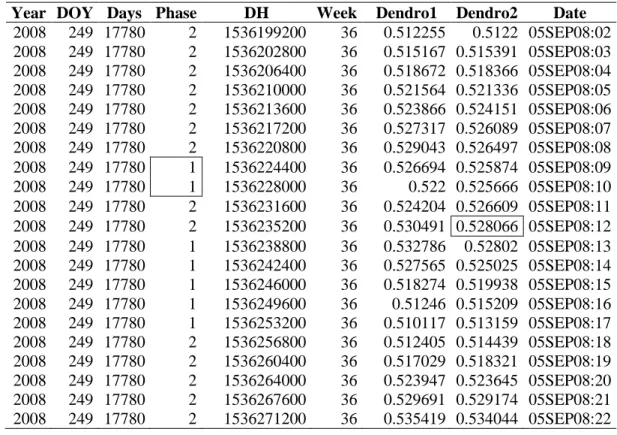
Year DOY Days Phase DH Week Dendro1 Dendro2 Date
2008 249 17780 2 1536199200 36 0.512255 0.5122 05SEP08:02 2008 249 17780 2 1536202800 36 0.515167 0.515391 05SEP08:03 2008 249 17780 2 1536206400 36 0.518672 0.518366 05SEP08:04 2008 249 17780 2 1536210000 36 0.521564 0.521336 05SEP08:05 2008 249 17780 2 1536213600 36 0.523866 0.524151 05SEP08:06 2008 249 17780 2 1536217200 36 0.527317 0.526089 05SEP08:07 2008 249 17780 2 1536220800 36 0.529043 0.526497 05SEP08:08 2008 249 17780 1 1536224400 36 0.526694 0.525874 05SEP08:09 2008 249 17780 1 1536228000 36 0.522 0.525666 05SEP08:10 2008 249 17780 2 1536231600 36 0.524204 0.526609 05SEP08:11 2008 249 17780 2 1536235200 36 0.530491 0.528066 05SEP08:12 2008 249 17780 1 1536238800 36 0.532786 0.52802 05SEP08:13 2008 249 17780 1 1536242400 36 0.527565 0.525025 05SEP08:14 2008 249 17780 1 1536246000 36 0.518274 0.519938 05SEP08:15 2008 249 17780 1 1536249600 36 0.51246 0.515209 05SEP08:16 2008 249 17780 1 1536253200 36 0.510117 0.513159 05SEP08:17 2008 249 17780 2 1536256800 36 0.512405 0.514439 05SEP08:18 2008 249 17780 2 1536260400 36 0.517029 0.518321 05SEP08:19 2008 249 17780 2 1536264000 36 0.523947 0.523645 05SEP08:20 2008 249 17780 2 1536267600 36 0.529691 0.529174 05SEP08:21 2008 249 17780 2 1536271200 36 0.535419 0.534044 05SEP08:22
Table 2. Output of the file p_filename.txt generated by the first SAS routine (Step 1)
containing the raw measurements (Dendro1), the trend-cycle component (Dendro2), a 390
variable classifying the phase of contraction and expansion (Phase) and additional descriptive variables of date (Days, DH, Week and Date).The maximum of the cycle occurring on 5 September 2008 takes place at 1200. The hours needing reclassification of the phase, by changing label 1 with 2 in the phase column, correspond to 0900 and 1000. The changes are made in a copy of this file p_filename_2.txt.
TABLE 3
Year DOY Hour Temp P Parm3 Parm4
2008 175 4 13.65 0.1 94.9 10.52017 2008 175 5 13.16 0.1 96.3 10.5003 2008 175 6 12.85 0 95.7 10.44051 2008 175 7 13.19 0 92.1 10.4126 2008 175 8 15.25 0 84.9 10.41622 2008 175 9 17.07 0 79.1 10.44283 2008 175 10 19.1 0 69.6 10.51451 2008 175 11 20.39 0.1 64.1 10.68244 2008 175 12 . 0 55 10.90359 2008 175 13 . 0 47.2 11.13717 2008 175 14 . 0 49.6 11.34054 2008 175 15 21.48 0 53.6 11.51155 2008 175 16 20.85 0 55.5 11.60849 2008 175 17 19.43 0 66.5 11.66297 2008 175 18 18.64 0 73.8 11.68004 2008 175 19 18.05 0 69.8 11.64752 2008 175 20 15.45 0.2 77.4 11.59628 2008 175 21 13.52 0.4 88.5 11.5286 2008 175 22 13.42 0 86.6 11.43293 2008 175 23 13.98 0 79.6 11.31925 2008 176 0 13.87 0 78.9 11.24421 2008 176 1 12.81 0 . 11.1567 2008 176 2 12.74 0 . 11.07005 2008 176 3 13.71 0 . 11.00994 2008 176 4 13.39 0 85.9 10.95529 2008 176 5 13.35 0 86.5 10.88533 2008 176 6 13.55 0 87.6 10.84383 2008 176 7 13.72 0 89.7 10.81669 2008 176 8 13.53 0.5 93.3 10.80078 2008 176 9 13.18 1.4 95.7 10.79641 2008 176 10 12.82 0.4 96.3 10.79986 2008 176 11 12.45 0.1 97 10.78135 2008 176 12 12.87 0 96.6 10.77737 2008 176 13 13.27 0 94.3 10.80048 2008 176 14 14.43 0 86.2 10.8519 2008 176 15 14.38 0 82.2 10.90764 2008 176 16 16.74 0 68.8 10.97474
Table 3. Example of an input meteorological dataset covering two partial days. The first
two meteorological parameters are hourly mean temperature (Temp, °C) and sum of precipitation (P, mm). Parm3 and Parm4 represent relative humidity (%) and soil 400
temperature (°C), respectively. Hours are formatted with two digits, without minutes. Missing data are replaced by dots.
TABLE 4
Cycle Days DOY Phase Nb MDS DeltaR Exp Temp Parm3 Parm4 Tmin Tmax SumP SumDeltaR
63 03-Jun-08 155 1 13 0.060392 -0.02118 0.039207 11.53615 64.77692 7.239809 5.3 14.43 0 -0.07523 64 04-Jun-08 156 1 11 0.067997 -0.01321 0.054782 12.50636 39.64545 6.670048 2.52 17.1 0 -0.08844 65 05-Jun-08 157 1 11 0.074304 -0.013 0.061304 16.46727 34.12727 6.997477 5.49 21.32 0 -0.10144 66 06-Jun-08 158 1 8 0.03362 0.027873 0.061493 19.28875 61.15 8.238629 15.92 22.06 0 -0.07357 67 07-Jun-08 159 1 10 0.061417 0.001981 0.063398 23.633 65.45 9.883481 16.11 26.74 0 -0.07159 68 08-Jun-08 160 1 5 0.018622 0.011696 0.030318 22.272 70.6 11.14408 19.69 23.42 0 -0.05989 69 09-Jun-08 161 1 8 0.048147 0.021638 0.069785 17.69 55.4875 10.04621 11.73 21.31 0 -0.03825 70 10-Jun-08 162 1 8 0.037157 0.034106 0.071263 22.92625 73.1875 10.75129 17.3 26.76 0 -0.00415 71 11-Jun-08 163 1 7 0.005033 -0.00317 0.001865 10.94571 91.41429 10.67668 9.21 12.9 0 -0.00732 72 12-Jun-08 164 1 14 0.066741 -0.02215 0.04459 12.15 60.24286 9.629385 6.05 17.32 0 -0.02947 73 13-Jun-08 165 1 10 0.07006 -0.01073 0.059327 19.25 33.81 9.323248 8.25 24.44 0 -0.0402 74 14-Jun-08 166 1 9 0.065843 0.092223 0.158066 21.90556 26.96667 10.18124 12.71 26.62 0 0.052023 75 16-Jun-08 168 1 6 0.022572 0.048028 0.070601 16.75833 82.6 10.03169 12.57 19.24 0.1 0.100052 76 18-Jun-08 170 1 6 0.017253 0.000244 0.017497 14.71 88.15 10.17387 12.34 16.23 5.9 0.100296 77 19-Jun-08 171 1 10 0.029768 0.004808 0.034575 14.785 79.42 10.01488 13.3 16.37 0.7 0.105103 78 20-Jun-08 172 1 10 0.015043 0.001518 0.016562 14.614 88.41 9.953514 13.85 15.58 1.9 0.106622 79 21-Jun-08 173 1 5 0.010895 0.023986 0.03488 15.2 87.62 9.760801 12.18 17.21 2.1 0.130607 80 22-Jun-08 174 1 7 0.030242 -0.00306 0.027184 16.67143 88.32857 10.00648 12.81 20.02 0.1 0.127549 81 23-Jun-08 175 1 10 0.058576 0.014815 0.073391 18.667 69.09 10.7802 12.85 22.94 0.1 0.142364
Table 4. Output of the file filename_phase1.txt generated by the second SAS routine (Step 3). The time series calculated for phase 1
are number of hours of contraction (Nb, h), maximum daily shrinkage (MDS, mm), net positive or negative increment (R, mm), stem
expansion (Exp, mm) and continuous sum of R (SumDeltaR, mm). The environmental parameters during contraction represent mean
temperature (Temp, °C), mean relative humidity (Parm3, %), mean soil temperature (Parm 4), minimum temperature (Tmin, °C), maximum temperature (Tmax, °C) and total precipitation (SumP, mm).
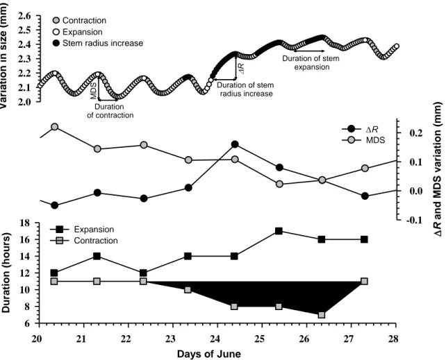
FIGURE 1 R an d M DS v ar iati on (mm) -0.1 0.0 0.1 0.2 R MDS Days of June 20 21 22 23 24 25 26 27 28 Durati on (hour s) 6 8 10 12 14 16 18 Expansion Contraction V ar iati on in si ze (mm) 2.0 2.1 2.2 2.3 2.4 2.5 2.6 Contraction Expansion
Stem radius increase
R Duration of stem radius increase Duration of contraction M DS Duration of stem expansion
Figure 1. Upper part: The stem cycle divided into three distinct phases of contraction
(grey dots), expansion (white and black dots) and stem radius increase (black dots). Middle part: net positive or negative increment (R, black dots) and maximum daily
shrinkage (MDS, grey dots) variations calculated with the stem cycle approach. Lower part: Duration (hours) of the phase of contraction (grey squares) and expansion (black squares).
FIGURE 2 Dataset (txt) Meteo data (txt) Partial dataset (txt) Partial dataset_2 (txt) Final datasets (txt) Plots (html) Submit Checking graphs Data processing Manual corrections Data processing Select filename, smoothing, days to enlarge
Submit Step 1 Measurements in the field Outputs Step 2 Step 3
Figure 2. Diagram of the three-step procedure to analyze the time series from an
FIGURE 3
Figure 3. Comparison between raw measurements (mm, dots) and the trend-cycle
component (mm, line) generated by the EXPAND procedure in SAS, with a 4-degree smoothing. The plot is automatically generated by the first SAS routine (Step 1) in a HTML-file (filename.html) referencing gif-format images. The y axis has no unit as these can differ between users.
FIGURE 4
Figure 4. Stem radius variation (mm) of Picea mariana recorded from spring to autumn
2008. The plot is automatically generated by the first SAS routine (Step 1) in a HTML-file (HTML-filename.html) referencing gif-format images. The y axis has no unit as these can differ between users.
FIGURE 5
Figure 5. Plot of hourly stem radius variation (mm) separated as contraction (black bars)
and expansion (grey bars). The plot is automatically generated by the first SAS routine (Step 1) in a HTML-file (filename.html) referencing gif-format images. The y axis has no unit as these can differ between users.
FIGURE 6
Month (2008)
Apr May Jun Jul Aug Sep Oct Nov
Sum of R (mm ) -0.2 0.0 0.2 0.4 M D S (m m ) 0.00 0.05 0.10 0.15 R (mm ) -0.10 -0.05 0.00 0.05 0.10
Figure 6. Stem variations of Picea mariana expressed as R, MDS and the sum of the
R’s over the whole period. The time series were generated by the second SAS routine
APPENDIX A
*SECTION 1: Define filename, smoothing degree and days to enlarge; %macro assegna;
%global smooth location name prima dopo; %let smooth=4;
%let location=C:\DendroUQAC; %let name=;
%let prima=170; %let dopo=175;
%window start irow=10 rows=12 icolumn=15 columns=45 color=black #1 @5 'DEPARTEMENT DES SCIENCES FONDAMENTALES' color=cyan
autoskip=yes protect=yes
#2 @7 'University of Quebec in Chicoutimi' color=cyan autoskip=yes protect=yes
#4 @4 "Filename" color=yellow +8 name 20 color=white required=yes #5 @4 "Smoothing value" color=yellow +1 smooth color=white
required=yes
#6 @4 "Days to enlarge" color=yellow +1 prima 3 color=white required=yes "-" color=white dopo 3 color=white required=yes; %display start;
%mend assegna; %assegna;
*SECTION 2: Import dataset; option noxwait;
%sysexec md "&location\&name";
%sysexec md "&location\&name\plots_&name"; %sysexec md "&location\&name\partial_&name"; data dendro1;
infile "&location\&name..txt" dlm=tab firstobs=2 expandtabs missover; input Year DOY hour dendro1; run;
proc sort data=dendro1; by DOY hour; run; data dendro2; set dendro1;
datejuli=(Year*1000)+DOY; Days=datejul(datejuli); minute=0;second=0;
DH=dhms(Days,hour,minute,second);
format DH datetime12.; drop datejuli minute second; run; *SECTION 3: ARIMA replacing missing values;
data miss1; set dendro2;
if dendro1 NE . then conta+1; run;
proc means data=miss1 noprint; by conta; var dendro1;
output out=miss2(drop=_TYPE_ _FREQ_) nmiss=miss; run; data miss3; merge miss1 miss2; by conta; run;
data miss4; set miss3;
if dendro1 NE . then miss=0; run;
proc arima data=miss4 out=arim; where miss<25; *missing data for less than one day;
identify var=dendro1(1,24) noprint;
estimate p=(2 0)(24) q=(0 1) noint method=cls noprint; forecast lead=0 id=DH noprint; run; quit;
if dendro1=. then dendro1=forecast; keep Year DH Days DOY dendro1; run; *SECTION 4: Fitting spline;
proc expand data=dendro3 out=spline;
convert dendro1=dendro2/transformout=(cd_tc &smooth); convert dendro1=s/transformout=(cda_s &smooth);
convert dendro1=i/transformout=(cda_i &smooth); convert dendro1=sa/transformout=(cda_sa &smooth); id DH; run;
data dendro4; set spline;
if dendro1=. then dendro2=.; run;
*SECTION 5: Compare maximum and minimum values and classify phases 1 and 2;
proc expand data=dendro4 out=dendro5;
convert dendro2=tc_m1h/ transform=(lead 1); convert dendro2=tc_p1h/ transform=(lag 1); convert dendro2=tc_p2h/ transform=(lag 2); id DH; run;
proc means data=dendro5 noprint; by Days; var dendro2;
output out=mxmn (drop=_freq_ _type_) max=mx min=minimo; run; data dendro6; merge dendro5 mxmn; by Days; drop s i sa; run; data cycle; set dendro6;
if dendro2 LE tc_p1h then Phase=1;
if dendro2=tc_p1h and dendro2 GT tc_p2h then Phase=2; if dendro2 EQ mx then Phase=2;
if dendro2 GE tc_p1h then Phase=2;
if dendro2=tc_p1h and dendro2 LT tc_p2h then Phase=1; drop tc_m1h tc_p1h tc_p2h mx minimo;
dh2=DH; rename DH=Date; rename dh2=DH; Week=ceil(DOY/7); run;
proc sort data=cycle; by Week; run; *SECTION 6: Export graphs;
filename odsout "&location\&name\plots_&name"; ods listing close;
ods html body="&name..html" path=odsout;
goptions device=gif reset=global gunit=pct border colors=(black red) ctext=black ftext=swiss htext=3;
title1 height=5 "Variations in size for &name";
footnote color=DAGRAY height=2.5 j=r "&sysday, &sysdate9 - Departement de Sciences Fondamentales - University of Quebec in Chicoutimi "; symbol1 V=none c=black i=join;
axis1 label=(h=4 font=arial "Date") value=(h=2.5 font=arial);
axis2 label=(h=4 font=arial angle=90 "Variation in size") value=(h=2.5 font=arial);
proc gplot data=dendro3;
plot dendro1*DH/haxis=axis1 vaxis=axis2 name='pattern'; run; quit; goptions;
symbol1 v=dot c=black i=join height=2; symbol2 v=none c=red i=join width=2;
proc gplot data=dendro4; where &prima<DOY<&dopo;
plot (dendro1 dendro2)*DH/overlay haxis=axis1 vaxis=axis2 name='smooth'; run; quit;
goptions;
title1 height=5 "Hourly variations for &name"; symbol1 c=black v=none i=needle width=2;
symbol2 c=red v=none i=needle width=2;
axis1 label=(h=4 font=arial) value=(h=2.5 font=arial);
axis2 label=(h=4 font=arial angle=90 "Variation in size") value=(h=2.5 font=arial);
proc gplot data=cycle; by week;
plot dendro2*Date=phase/haxis=axis1 vaxis=axis2 nolegend name='plot'; run; quit;
ods html close;
*SECTION 7: Export dataset; data cycle2; set cycle;
Dendro11=Dendro1; Dendro22=Dendro2; format date2 datetime12.; date2=Date; drop Date dendro1 dendro2;
rename date2=Date dendro11=Dendro1 dendro22=Dendro2 jh2=DH; if dendro1=. then dendro1=dendro2;
if dendro2=. then delete; run; proc export data=CYCLE2
outfile="&location\&name\partial_&name\p_&name..txt" DBMS=TAB REPLACE; run;
data _null_;
call sound(600,40); call sound(700,40); call sound(800,40);
APPENDIX B
*SECTION 1: Define filename; %macro assegna;
%global location name meteo; %let location=C:\DendroUQAC; %let name=;
%let meteo=;
%window start irow=10 rows=12 icolumn=15 columns=45 color=black #1 @5 'DEPARTEMENT DES SCIENCES FONDAMENTALES' color=cyan
autoskip=yes protect=yes
#2 @7 'University of Quebec in Chicoutimi' color=cyan autoskip=yes protect=yes
#4 @4 "Foldername" color=yellow +4 name 20 color=white required=yes #6 @4 "Meteodata" color=yellow +5 meteo 20 color=white required=yes; %display start;
%mend assegna; %assegna;
*SECTION 2: Import dataset; option noxwait;
%sysexec md "&location\&name\final_&name"; data cycle0;
infile "&location\&name\partial_&name\p_&name._2.txt" dlm=tab firstobs=2 missover expandtabs;
input Year DOY Days Phase DH Week Dendro1 Dendro2; format dh datetime12.;
lag=LAG(phase); run; data meteo;
infile "&location\&meteo..txt" dlm=tab firstobs=2 missover expandtabs;
input Year DOY Hour Temp P Parm3 Parm4 Parm5 Parm6 Parm7 Parm8; datejuli=(year*1000)+DOY;
days=datejul(datejuli); minute=0;second=0;
dh=dhms(days,hour,minute,second); drop datejuli minute second; run; proc sort data=cycle0; by dh; run; proc sort data=meteo; by dh; run;
data cycle1; merge cycle0 meteo; by dh; run; *SECTION 3: Cycle definition;
data cycle2; set cycle1; conta+1;
if lag NE phase then conta=1; drop lag; run;
data cycle4; set cycle2;
retain Cycle 1; if phase=1 and conta=1 then Cycle=Cycle+1; drop conta; run;
*SECTION 4: Assess phases and timings; data cycle5; set cycle4;
var Dendro2; id year;
output out=cycle6 (drop=_freq_ _type_) max=massimo; run;
proc expand data=cycle6(where=( cycle NE .)) out=cycle7(drop=TIME); convert massimo=max_lag/ transform=(lag 1); run;
proc sort data=cycle4; by cycle; run; proc means data=cycle4 noprint; by cycle; var Dendro2; id year;
output out=cycle8 (drop=_freq_ _type_) min=minimo; run; data cycle_01; merge cycle4 cycle7; by cycle;
hour=hour(dh); run;
data cycle9; merge cycle_01 cycle8; by cycle; if phase=2 and Dendro2 GT max_lag then phase=3; MDS=max_lag-minimo; if MDS<0 then MDS=0.00001; DeltaR=massimo-max_lag;
EXP=massimo-minimo;
if phase=. then delete; run;
*SECTION 5: Calculate means for each phase;
proc means data=cycle9(where=(phase NE 2) ) noprint; by cycle phase; var MDS DeltaR EXP Temp P parm3 parm4 parm5 parm6 parm7 parm8;
output out=X1 (drop=_freq_ _type_ z1-z11) n=Nb
mean=MDS DeltaR Exp Temp Z1 Parm3 Parm4 Parm5 Parm6 Parm7 Parm8 min=Z2 Z3 Z4 Tmin max=Z5 Z6 Z7 Tmax sum=Z8 Z9 Z10 Z11 SumP; run; proc sort data=X1; by cycle phase; run;
proc means data=cycle9(where=(phase=2) ) noprint; by cycle phase; var MDS DeltaR EXP Temp P parm3 parm4 parm5 parm6 parm7 parm8; output out=X2 (drop=_freq_ _type_ z1-z11) n=Nb
mean=MDS DeltaR Exp Temp Z1 Parm3 Parm4 Parm5 Parm6 Parm7 Parm8 min=Z2 Z3 Z4 Tmin max=Z5 Z6 Z7 Tmax sum=Z8 Z9 Z10 Z11 SumP; run; proc sort data=X2; by cycle phase; run;
proc means data=cycle9 noprint; by cycle;
var MDS DeltaR EXP Temp P parm3 parm4 parm5 parm6 parm7 parm8; output out=X3 (drop=_freq_ _type_ z1-z11) n=Nb
mean=MDS DeltaR Exp Temp Z1 Parm3 Parm4 Parm5 Parm6 Parm7 Parm8 min=Z2 Z3 Z4 Tmin max=Z5 Z6 Z7 Tmax sum=Z8 Z9 Z10 Z11 SumP; run; data x3; set x3; phase=4; run;
*SECTION 6: Merge all datasets;
proc sort data=X3; by cycle phase; run; run; data analyse2; merge x1 x2 x3; by cycle phase; proc sort data=analyse2; by cycle phase; run; proc means data=cycle9 noprint; by cycle; var days DOY;
output out=days (drop=_freq_ _type_) mean=Days DOY; run; proc expand data=x3 out=sum (keep=cycle SumDeltaR); convert DeltaR=SumDeltaR/transform=(cusum 1); run; data analyse3; merge days analyse2 sum; by cycle;
Days=floor(days); format Days date9.; DOY=floor(DOY); run; *SECTION 7: Export datasets;
proc export data=analyse3
outfile="&location\&name\final_&name\final_&name..txt" DBMS=TAB REPLACE; run;
%macro esporta; %do phase=1 %to 4;
proc export data=phase&phase outfile="&location\&name\final_&name\&name._phase&phase..txt" DBMS=TAB REPLACE; run; %end; %mend esporta; %esporta; data _null_;
call sound(600,40); call sound(700,40); call sound(800,40);