HAL Id: hal-00298329
https://hal.archives-ouvertes.fr/hal-00298329
Submitted on 4 May 2007
HAL is a multi-disciplinary open access
archive for the deposit and dissemination of
sci-entific research documents, whether they are
pub-lished or not. The documents may come from
teaching and research institutions in France or
abroad, or from public or private research centers.
L’archive ouverte pluridisciplinaire HAL, est
destinée au dépôt et à la diffusion de documents
scientifiques de niveau recherche, publiés ou non,
émanant des établissements d’enseignement et de
recherche français ou étrangers, des laboratoires
publics ou privés.
objects: applications in MFSTEP
C. Pizzigalli, V. Rupolo
To cite this version:
C. Pizzigalli, V. Rupolo. Simulations of ARGO profilers and of surface floating objects: applications
in MFSTEP. Ocean Science, European Geosciences Union, 2007, 3 (2), pp.205-222. �hal-00298329�
www.ocean-sci.net/3/205/2007/
© Author(s) 2007. This work is licensed under a Creative Commons License.
Ocean Science
Simulations of ARGO profilers and of surface floating objects:
applications in MFSTEP
C. Pizzigalli and V. Rupolo
Climate Department, ENEA, Via Anguillarese 301 00060 Rome, Italy
Received: 5 October 2006 – Published in Ocean Sci. Discuss.: 20 October 2006 Revised: 19 March 2007 – Accepted: 5 April 2007 – Published: 4 May 2007
Abstract. In this work we describe part of the activities
performed in the MFSTEP project by means of numerical simulations of ARGO profilers and surface floating objects. Simulations of ARGO floats were used to define the optimal time cycling in order to maximize independent observations of vertical profiles of temperature and salinity and to mini-mize the error on the estimate of the velocity at the parking depth of the profilers. Instead, the Mediterranean Forecasting System archive of Eulerian velocity field from 2000 to 2004 was used to build a related surface Lagrangian archive, sys-tematically integrating numerical particles released and con-strained to drift at surface. Here we use such Lagrangian archive to study the interannual variability of the surface La-grangian transport in two key areas of the Western Mediter-ranean, also introducing an exponential decay in the particles concentration.
1 Introduction
The Eulerian description of the flow is obviously of primary importance for the knowledge of the dynamics of the sea, but often critical questions concerning the path of the water masses are much more easily accessible from the Lagrangian picture of the motion. Moreover, Lagrangian experimental devices provide economical observations over extended ar-eas for long time periods, even during extreme weather con-ditions, and play by now a major role in the global ocean observing system. These simple observations have moti-vated, as one important enrichment of the general architec-ture of the previous Mediterranean Forecasting System Pilot Project (MFSPP), the introduction of the Lagrangian frame-work, both in the modelling and observing part of MFSTEP.
Correspondence to: V. Rupolo
During the project, starting from June 2004, about twenty autonomous drifting ARGO profilers were deployed in the Mediterranean Sea in the context of the MedARGO project that is fully described in the papers of Poulain (2005) and Poulain et al. (2006). ARGO floats freely drift at a prescribed depth for a given time interval and then they resurface and transmit to the satellite ARGOS system position data and ver-tical Temperature and Salinity (TS) profiles, before starting a new cycle. In the global oceans, data from autonomous drift-ing profilers are collected in the framework of the ARGO international project (http://www.argo.net) as a part of the global ocean observing system whose main aim is to col-lect data to detect and study climate changes. ARGO vertical profiles are collected typically at 10 days interval in the up-per 2000 m. Contrastingly, MedARGO data are collected to provide Near Real Time (NRT) TS data to be assimilated, to-gether with the Temperature profiles from the Volunteer Ob-serving Ships (Manzella et al., 2003), in an operational fore-casting model of a basin of reduced size and characterized by a rather complex bathymetric structure. Other than TS ver-tical profiles, autonomous drifters profilers provide also in-formation about the velocities at the parking depth that may also be assimilated in a General Circulation Model (Molcard et al., 2005). However, this estimate, being obtained directly from the resurfacing positions of the ARGO profilers, do not consider residual motions at intermediate depth and it is af-fected by the intrinsic errors given by the neglected horizon-tal displacements during the vertical motion of the profiler. Consequently, designing the overall MFSTEP architecture it was foreseen a research activity devoted to define, by means of numerical simulations, the ‘best’ cycling characteristics for the MedARGO floats in order to maximize independent observations of vertical profiles of TS and to study the er-ror on the estimate of intermediate velocity, its dependence on the time characteristics of the profiler cycle and, possibly, on the geographic area of release. The technique adopted for these purposes is described in detail in this paper, while
in Poulain et al. (2006) only the results are presented. Dur-ing MFSTEP, numerical simulations of the ARGO profilers movement were also used to quantify the impact of assim-ilating in the forecasting model vertical TS profiles (Griffa et al., 2006; Raicich 2006) and positions (Taillandier and Griffa, 2006) and to design an array of profiling floats for the estimation of the 3-D thermohaline fields (Guinehut et al., 2002).
Eulerian velocity fields from MFSPP were also used to compute numerical trajectories to study in the Mediterranean the variability of the surface dispersion, since a better de-scription of its phenomenology is an important oceano-graphic issue both for operational and scientific purposes. For operational purposes, the knowledge of surface disper-sal properties is useful in case of pollutant releases at sea (e.g. oil spill), for the assessment of biological quantities such as larvae spreading and in the search and rescue ac-tivities, to make a first guess at the most probable direction of drifting. For scientific purposes, information about the Lagrangian dispersion variability at sea surface is an appro-priate tool to study the heat and salt budgets in an evapora-tive basin like the Mediterranean Sea, where the hydrological properties of the surface layers often considerably differ from those of the sub-surface layers and where, due to the pres-ence of geomorphic constraints, the variability of the surface flow may influence the basin-wide thermohaline circulation through modification of the heat and salinity contents (As-traldi et al., 1992). Technically, using MFSPP Eulerian
hind-cast velocity fields from the 2000 to 2004, we have built a
huge Lagrangian archive systematically integrating particles released, and constrained to drift, at surface. This “Lagra-nian atlas”, obtained from velocity fields in which the effects of the variability of the surface forcing is fully represented, was already used to study, following a statistical approach, the seasonal variability of surface dispersion at basin scale (Pizzigalli et al., 2007). In this work we present a further ex-ample of exploitation of this Lagrangian data set investigat-ing the interannual variability of the “Lagrangian transport” in two key areas of the Mediterranean Sea considering also the case of tracers characterized by a concentration decreas-ing with an exponential decay.
Numerical simulation of both ARGO profilers and surface floating objects were done using the basin wide Eulerian ve-locity fields from the Med831 model (MOM 1/8◦×1/8◦×31 levels, model details are described in Korres at al., 2000, and Demirov et al., 2003). Obviously, all the results pre-sented in this study depend on the performance of the Eu-lerian model. The scarce space and time resolution does not allows for a proper representation of the high-frequency sub inertial and mesoscale motions and among other model deficiencies (e.g. unsophisticated representation of sub-grid scale effects) likely causing discrepancies between real and modelled floating objects, one can mention the lack of a pa-rameterization representing the wave effects. Finally, the space resolution (about 0.5◦) of the ECMWF (European
Cen-tre for Medium-Range Weather Forecasts) analysis used to force the MFSPP OGCM may not be sufficient to properly represent the wind-induced surface dynamics especially in a basin in which the neighbouring lands are characterized by complex orography. However, the MFSPP Eulerian velocity fields used in this study, obtained from a model which assim-ilates in-situ real data and is forced by analyzed wind fields, represent the best basin scale description one can get for the variability of the circulation patterns from the model grid size scale h to the Mediterranean sub-basins scale, whose typical dimension is of the order of 300–500 km, i.e. for times t:
h
V≈1 day<t<
300−500 km
V ≈30 days, where V ≈10 cm/s is the
typical scale of velocity.
Comparing numerical and real Lagrangian trajectories is perhaps one of the most stringent model validation proce-dure. When dealing with ARGO simulations we will com-pare some statistical properties of the cycles of numerical and real MedARGO profilers, which may be considered as an in-direct validation procedure to check the ability of the OGCM to represent subsurface flow. In Pizzigalli et al. (2007) we check the results obtained from a seasonal statistics of numerical surface dispersion with experimental data from the Mediterranean Surface Drifter Database (Poulain et al., 2004) showing that the MFSPP OGCM reasonably well rep-resent the variability of dispersion in such time scales (from few days to few weeks). The results presented here con-cerning the interannual variability of the surface Lagrangian transport in the Corsica and Sardinia Channels may hardly be checked against real data. However, this “intra-basin” trans-port occurs on space and time scales well resolved by the model and it is mainly driven by atmospheric features whose relatively low space and time variability is well represented in the ECMWF wind fields. We consequently believe that the results presented here, possibly compared with other nu-merical studies and when possible with real Lagrangian data, may be still be useful to study and assess the variability of the surface circulation in the Mediterranean Sea.
This work is composed by two different and separate parts. In Sect. 2 we describe in detail the use of the numerical simu-lations of the ARGO profilers for the definition of the optimal sampling strategy and we discuss the statistics of the errors on the determination of the sub-surface velocity from ARGO data. In Sect. 3 we show some results concerning the inter-annual variability of the Lagrangian transport in the Corsica and Sardinia Channels taking also into account the dilution rate of the tracer due, e.g., to the evaporation of the given pollutant or to the larvae mortality. Finally, Sect. 4 summa-rizes the results and discusses some future prospects, notably in terms of development and improvement of the use of La-grangian numerical tools in operational projects.
2 Numerical ARGO profilers
2.1 Numerical algorithm
The motion of the profiler is simulated through an off-line algorithm obtained modifying the original code ARIANE (http://www.ifremer.fr/lpo/blanke/ARIANE/index. html; Blanke and Raynaud, 1997). During a profiler cycle (see Fig. 1) the simulated profiler downwells to a specified depth Zdrift, where it freely drifts for a given time Tdrift,
then further downwells to a second specified depth Zdown
to immediately upwells to the surface, where it stays for a given time Tsurf. During the vertical displacements the
floats are subjected to the horizontal movements induced by the vertical velocity shear. For the real profilers of the MedARGO program the “parking” depth Zdrift was
cho-sen to be fixed at 350 m, that approximately corresponds to the “mean core depth” of the Levantine Intermediate Wa-ter, while the deepest depth is fixed at 700 m (Poulain et al., 2006). For some floats and every ten cycles the floats down-wells to a depth Zdown=2000 m. In each numerical
experi-ment the parking and the deepest depths were fixed at 350 m and at 700 m, (for all the cycles), while, during the verti-cal displacements, the “numeriverti-cal profilers” move with the constant experimental-like downward and upward velocities w=−5 cm/s and w=10 cm/s, respectively.
In each cycle the profiler stays at surface for a time Tsurf=Tsurf1+Tsurf2+Tsurf3 where Tsurf1=Tsurf2≈15 min
rep-resent, respectively, the time intervals between the last sur-face positioning and the sinking and between the resurfacing and the first satellite positioning of the float and Tsurf3≈6 h is
the time spent at surface to transmit data. The time interval Ttotbetween the last float positioning in the surface and the
first positioning after the re-surfacing is given (see Fig. 1) by: Ttot= Tsurf1+ Tdown1+ Tdrift+ Tdown2+ Tupw+ Tsurf2,
where Tdown1=Tdown2=5 cm/s350 m≈2 h is the time necessary for
the first (from surface to 350 m) and the second (from 350 to 700 m) upwelling and Tupw=10 cm/s700 m ≈2 h is the time
neces-sary for the upwelling of the profiler to the surface. During the horizontal and vertical movements the profiler trajectory is sampled every 3 h and every 18 s, respectively. The code is flexible and the user can easily change the depth and the time characteristics of the cycles.
2.2 Numerical experiments and cycles statistics
We have performed 6 experiments varying the time Tdrift
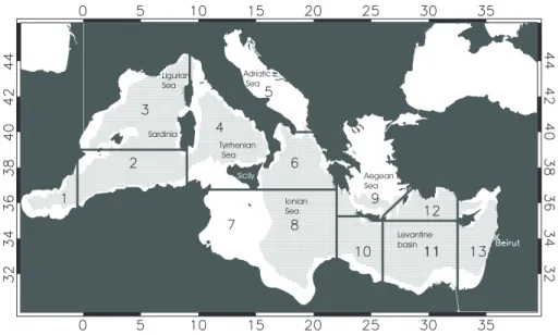
from 3 to 30 days. In each experiment 40 136 “numerical profilers” are uniformly released at surface (with an approx-imate density of 4 particles/100 km2) only where the bottom sea is deeper than 700 m, with the exceptions of the shallow North Aegean, Adriatic Sea and Sicily Channel (see Fig. 2). After the release each numerical profiler sinks to the equilib-rium depth of 350 m and starts its cycles. The integration is
Fig. 1. Schematic and notations used in the text for a typical profiler cycle.
performed for 364 days using the 3 days mean eulerian
hind-cast velocity field of the year 2000 (52 weeks) obtained with
the Med831 model (MOM 1/8◦×1/8◦×31, see Korres at al., 2000, and Demirov et al., 2003).
When a real ARGO float crashes on the bottom it simply stays at the floor sea for the described time and then it resur-faces. In our simulations, if the numerical profiler reaches the bottom it immediately resurfaces to start a new cycle and, to avoid spurious results, we consider in our statistics only cy-cles in which the numerical floats do not reach the bottom. Consequently we have a statistics based on a number of cy-cles Ncycles6=Nt c=Npart·TTINTtot , where Npart is the number of
profilers and TINT=364. For each experiment Ncycles is
al-ways very large (see Table 1) and the ratio NNcycles
t c is about
0.66 for EXP1 and about 0.75 for the five experiments EXP2-EXP6. From 2004 to the end of 2006 are available 1791 cy-cles of MedARGO floats with 4.5 days<TTot<5.5 days (for
real MedARGO floats Tdrift=5 days), that were downloaded
from the ARGO Data Center. The ARGO netcdf files contain for each float cycle a parameter indicating, when known, if the float has touched the ground. Unfortunately for more than 80% of cycles this parameter results to be “unknown” mak-ing impossible a direct comparison of the percentage of cy-cles touching the sea floor between numerical and real data.
Fig. 2. Numerical profilers are uniformly released at surface in the grey light area. Numbers indicate the different regions discussed in the text.
Table 1. Tdrift, total number of cycles and number of cycles characterized by having |Xtot| greater than 10 and 20 km for MedARGO data
and the six numerical experiments. In each experiment were integrated 40 136 numerical profilers uniformly released at surface.
Tdrift(days) Ncycles |XTot|>10 |XTot|>20
MedARGO 5 1791 1190 (66%) 581 (32%) EXP1 3 3 207 232 1 913 600 (60%) 814 419 (25%) EXP2 6 1 809 631 1 323 463 (73%) 881 675 (49%) EXP3 9 1 229 731 1 006 347 (82%) 778 891 (63%) EXP4 12 917 250 798 536 (87%) 665 921 (73%) EXP5 15 739 580 668 086 (90%) 580 922 (79%) EXP6 30 365 745 350 905 (96%) 329 546 (90%)
However, we may obtain a rough estimate of the number of cycles touching the sea floor considering the points that lie in the band defined by the two lines ZMax=ZBot±|Err|, where
ZMaxis the deepest depth reached by the floats, ZBot is the
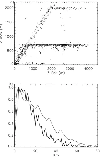
bottom depth at the location of the profile and the error Err may be due or to the indeterminacy of the position or to the discretised topography data set. Considering values of Err of 50 and 100 m, we have that about the 6% and 9% of the points of the scatter plot shown in Fig. 3a lie in such bands, which indicates that the numerical results overestimate the number of cycles in which the float touches the sea floor, even if it has to be stressed that many numerical profilers are released near the isobath of 700 m (Zdown=700 m).
In the two last columns of Table 1, we show the num-ber and percentages of cycles in which |XTot| is greater
than 10 and 20 km, which may be considered as a proxy of number of consecutive independent vertical profiles of TS, since the Rossby deformation radius that in the Mediter-ranean Sea is of the order of O(5–15) km. The percentage
of consecutive and independent observations tends to sat-urate to 100% only for very big Tdrift. For Tdrift=6 days
(EXP2) we have that about the 73% and 49% of cycles have |XTot| >10 and 20 km, respectively. The number of cycles
with |XTot| >10 km is greater for EXP1 while the number
of cycles with |XTot| >20 km, slightly larger for EXP2, is
almost similar for EXP1, EXP2 and EXP3. These results was used to define the time cycling characteristics of the real MedARGO floats, and it is encouraging to note that the nu-merical results are in general agreement with real data since the percentage of MedARGO cycles with |XTot| >10 and
20 km lies between results from EXP1 and EXP2 (see also Fig. 3b).
Fig. 3. Panel (a) scatter plot of maximum depth of experimental Medargo cycles (1791) vs. bottom depth at the resurfacing location. Bottom depth is retrieved from the Digital Bathymetric Data Base at 1′ resolution and was kindly provided by M. Tonani (INGV). Dotted and dashed lines are defined by ZMax=ZBOT±|Err| with
Err=50 m and Err=100 m, respectively. Panel (b) Histogram of dis-tance between two subsequent resurfacing locations for EXP2 and MedARGO real data (thin and thick line, respectively). We consider only real cycles which passed all automatic quality control test and separated by a time interval 4.5 days<TTot<5.5 days.
2.3 Sub-surface velocities
The estimate of the intermediate currents by means of ARGO floats is given by U = XTot Ttot = X2− X1 Ttot , (1)
where Xi are the surface positions before and after the deep cycle of the float and Ttotis the time interval between these
two subsequent, satellites located, surface points (see Fig. 1). This estimate (Eq. 1) is inadequate when Tdriftis greater or
comparable to the intermediate velocity Lagrangian
corre-Table 2. Percentage of cycles characterized by a ratio|Xdrift| D <L. L=0.9 L=0.8 L=0.7 L=0.6 EXP1 2% 1% <1% <1% EXP2 6% 3% 1% 1% EXP3 13% 6% 2% 2% EXP4 21% 10% 4% 3% EXP5 29% 15% 6% 4% EXP6 57% 37% 18% 13%
lation time TL since in this case, due to the presence of eddies and meanders, the length of the piece of trajectory D=RTj+Tdrift
Tj dY covered by the profiler in the time Tdriftis
greater than Xdrift = Y2−Y1
, where Yi represent coordi-nates of the first and last point of the trajectory at the parking depth Zdrift. A second source of inaccuracy is given by the
fact that the definition (1) does not take into account the hori-zontal displacements occurring at the surface, first and before the satellite locations, and during the vertical motions of the profiler ( XTot 6=
Xdrift in the notation of Fig. 1).
We have then computead, for each cycle of the six ex-periments EXP1-EXP6, Xdrift and the distance D covered by the numerical profilers, approximated as a broken line of segments of time length equal to the time interval of the La-grangian integration (3 h). From Table 2, where we report for each experiment the percentage of cycles in which the ratio
|Xdrift|
D is smaller than a threshold value L, it is possible to see that a significant number of cycle (>5%) have an impor-tant difference (L<0.8) for Tdrift≥9 days, time scale that may
be considered as a crude estimate of the order of magnitude of TLfrom the numerical Lagrangian velocity time series at 350 m.
The same experiments are used to assess the role of the vertical velocity shear and surface motions computing for each cycle
XTot ,
Xdrift
and the error 1 on the estimate of the intermediate velocity that is defined as:
1(Tdrift) = XTot − Xdrift Xdrift . (2)
This huge statistics is then used to directly quantify the de-pendence of 1 on Tdriftand to define possible criteria to
de-crease the error (2) or to identify geographical area where the vertical shear gives raise to smaller error 1.
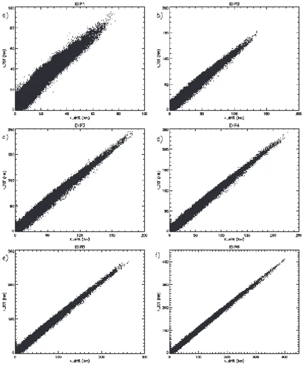
In Fig. 4 we show the scatter plot of XTot
vs. Xdrift
computed for each cycle of the six experiments. As is ex-pected, increasing Tdrif the plot is less “scattered” and the
correlation between Xdrift and
XTot is more pronounced. However, due to the existence in each experiment of cy-cles with small Xdrift , the corresponding mean errors are very high, the standard deviation of 1 largely exceeds its mean value and the probability density function (pdf) P (1)
Fig. 4. Scatter plot of |Xtot| vs. |Xdrift| for EXP1-EXP6 (panels a to f).
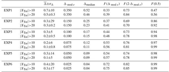
of 1 (Fig. 5) , even if characterized by well defined peak (“mode” value) for relatively low values of 1, has very long tails. Considering only cycles in which the surface displace-ment XTot is greater than 10 and 20 km the estimate on the intermediate velocity definitely improves. In Table 3 we report, for such cycles, mean and standard deviation of 1 and other statistical indices computed from the cumula-tive F ( ˆ1)=R1ˆ
0 P (1)d1, which represents the probability
to have a value 1< ˆ1. For instance if in EXP2 we consider only cycles with XTot >10 km (20 km) we have that 50% of
cycles have an error less than 0.25 (0.23) and that the 37%, 69% and 86% (41%, 70% and 92%) of cycles gives an esti-mate of the intermediate velocities with an error smaller than 0.15, 0.30 and 0.50 (F (1Mode), F (2·1Mode) and F (0.5)),
re-spectively. Neglecting cycles with small XTot (the only ex-perimental observable variable) is only a first guess in order to attempt to avoid floats with weak intermediate current. In a barotropic situation a small XTot implies a small
Xdrift and considering only cycles with XTot greater than a threshold value may help to avoid floats moving very slowly; however, in presence of strong shear it is possible to have small Xdrift
Table 3. Different statistical indices from the pdf of the error (1) from the six experiments.
1±σ1 1mod e 1median F (1mod e) F (2·1mod e) F (0.5)
EXP1 |XTot|>10 |XTot|>20 0.7±10 0.5±0.3 0.350 0.350 0.52 0.46 0.33 0.39 0.73 0.84 0.47 0.56 EXP2 |XTot|>10 |XTot|>20 0.3±29 0.3±0.2 0.150 0.150 0.25 0.23 0.37 0.41 0.69 0.70 0.86 0.92 EXP3 |XTot|>10 |XTot|>20 0.3±5 0.2±0.5 0.100 0.100 0.17 0.15 0.44 0.48 0.73 0.78 0.94 0.98 EXP4 |XTot|>10 |XTot|>20 0.2±6 0.1±0.8 0.075 0.075 0.12 0.11 0.53 0.56 0.76 0.81 0.97 0.99 EXP5 |XTot|>10 |XTot|>20 0.3±14 0.1±5 0.050 0.050 0.09 0.09 0.54 0.57 0.74 0.78 0.98 0.99 EXP6 |XTot|>10 |XTot|>20 0.4±20 0.3±17 0.025 0.025 0.04 0.04 0.72 0.75 0.82 0.85 0.99 0.99
Fig. 5. Pdf of 1 and its cumulative (dashed-dotted line) computed considering all the cycles for the four experiments EXP1-EXP4.
with large XTot . In Fig. 6 we show the pdf of 1 together with its cumulative computed considering only cycles with
XTot >20 km for the four experiments EXP1-EXP4. Obviously the error decreases when the time Tdrift
in-creases but since the primary aim of the MedARGO exper-iment was the collection of the maximum number of in-dependent TS vertical profiles, and since the assimilation procedure of positions in an OGGM requires that the park-ing time Tdrift≤TL, in the following we will analyze re-sults only from EXP1 and EXP2. In particular, to identify
Fig. 6. Pdf of 1 and its cumulative (dashed-dotted line) computed considering only cycles with
XTot
>20 km for the four
experi-ments EXP1-EXP4.
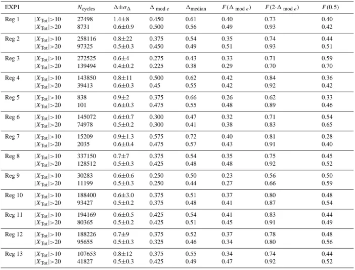
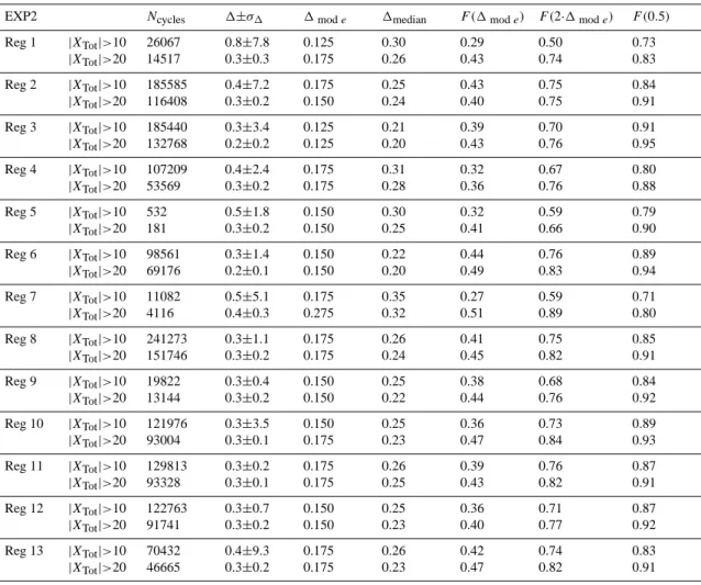
a possible dependence of 1 on the geographical position, we report in Tables 4 and 5 for such experiments the val-ues of ¯1±σ1, 1Mode, 1MedianF (1Mode), F (2·1Mode) and
F (0.5) computed considering cycles with XTot >10 km and 20 km in the 13 regions indicated in Fig. 2. For cycles with XTot >20 km, the standard deviation is smaller than the mean values almost everywhere and for EXP2 1Median
ranges from 0.20 (Regions 3 and 6) to 0.32 (Region 7) and we have that the probability of having an estimate of the
Table 4. EXP1: Ncycles, and statistical indices from the pdf of 1, in the different regions defined in Fig. 2.
EXP1 Ncycles 1±σ1 1mod e 1median F (1mod e) F (2·1mod e) F (0.5)
Reg 1 |XTot|>10 |XTot|>20 27498 8731 1.4±8 0.6±0.9 0.450 0.500 0.61 0.56 0.40 0.49 0.73 0.93 0.40 0.42 Reg 2 |XTot|>10 |XTot|>20 258116 97325 0.8±22 0.5±0.3 0.375 0.450 0.54 0.49 0.35 0.51 0.74 0.93 0.44 0.51 Reg 3 |XTot|>10 |XTot|>20 272525 139494 0.6±4 0.4±0.2 0.275 0.225 0.43 0.38 0.33 0.29 0.71 0.70 0.59 0.70 Reg 4 |XTot|>10 |XTot|>20 143850 39413 0.8±11 0.6±0.3 0.500 0.45 0.62 0.55 0.42 0.42 0.84 0.92 0.36 0.42 Reg 5 |XTot|>10 |XTot|>20 838 101 0.9±2 0.6±0.3 0.375 0.475 0.66 0.55 0.26 0.48 0.62 0.89 0.33 0.46 Reg 6 |XTot|>10 |XTot|>20 145072 74978 0.6±0.7 0.5±0.2 0.300 0.300 0.47 0.41 0.32 0.38 0.71 0.83 0.54 0.65 Reg 7 |XTot|>10 |XTot|>20 15209 2035 0.9±1.3 0.6±0.4 0.575 0.475 0.72 0.57 0.40 0.43 0.81 0.91 0.28 0.40 Reg 8 |XTot|>10 |XTot|>20 337150 128512 0.7±7 0.5±0.3 0.375 0.425 0.54 0.48 0.35 0.48 0.75 0.92 0.45 0.52 Reg 9 |XTot|>10 |XTot|>20 30283 11199 0.6±0.6 0.5±0.3 0.250 0.250 0.50 0.44 0.23 0.27 0.56 0.66 0.50 0.59 Reg 10 |XTot|>10 |XTot|>20 188400 93427 0.6±3.0 0.5±0.2 0.375 0.375 0.51 0.48 0.37 0.41 0.80 0.87 0.48 0.54 Reg 11 |XTot|>10 |XTot|>20 194169 80365 0.6±0.5 0.5±0.2 0.425 0.425 0.54 0.51 0.41 0.45 0.83 0.91 0.44 0.49 Reg 12 |XTot|>10 |XTot|>20 188226 95655 0.7±9 0.5±0.3 0.375 0.325 0.52 0.46 0.37 0.34 0.78 0.80 0.48 0.56 Reg 13 |XTot|>10 |XTot|>20 107653 41827 0.8±12 0.5±0.3 0.375 0.425 0.55 0.49 0.34 0.47 0.74 0.92 0.44 0.52
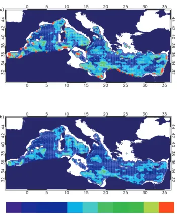
intermediate velocity with an error <0.5 (F(0.5)) varies from the 80% (Region 7) to the 95% (Region 3). This regional analysis shows that the estimate of the intermediate veloc-ities is characterized by a smaller error in the North West-ern Mediterranean Sea (NWM) in the NorthWest-ern Ionian (Re-gions 3 and 6) and in Western Levantine basin (Re(Re-gions 10 and 11) while the Tyrrhenian and the Adriatic Seas and the Sicily Channel are expected to be characterized by a larger error. In Fig. 7 we map for EXP2 the mean error 1 computed averaging, on a grid of 0.25◦×0.25◦, between all the error values of the cycles with XTot >10 km and XTot >20 km falling in a given bin. From this figure we can also see that the whole area north to the African coast (influenced by the flow of the Modified Atlantic Water which gives rise to a strong velocity shear) is characterized by a greater error on the estimate of the intermediate velocities.
Finally, in Fig. 8 we show, always for EXP2, the initial conditions of the numerical ARGO floats characterized by having 1<0.25, where now 1 is the mean error computed on all the cycles of the entire 1 year long trajectory. Except
some small scale features, like the spots in vicinity of the Sicily and Sardinia Channel, of difficult explanation, also the large scale picture of this figure indicates that numerical sim-ulations suggest that the NWM, the Ionian Sea together with the Levantine basin are favourite sites for the deployment of ARGO profilers in order to have smaller error on the estimate of sub-surface velocities.
We conclude this section noting that the analysis of nu-merical profilers other than indicating areas where one can expect a smaller error on the estimate of subsurface velocities were useful to define the parking time Tdriftfor the real
pro-filers that was finally chosen to be equal to 5 days (Poulain et al., 2006), since this values is as a good compromise be-tween the different and contrasting needs of having the larger number of independent observations, a small error on the es-timate of the intermediate velocities and a time length of the profiler cycle smaller than the intermediate velocities decor-relation time TL.
Table 5. EXP2: Ncycles, and different statistical indices from the pdf of 1, in the different regions defined in Fig. 2.
EXP2 Ncycles 1±σ1 1mod e 1median F (1mod e) F (2·1mod e) F (0.5)
Reg 1 |XTot|>10 |XTot|>20 26067 14517 0.8±7.8 0.3±0.3 0.125 0.175 0.30 0.26 0.29 0.43 0.50 0.74 0.73 0.83 Reg 2 |XTot|>10 |XTot|>20 185585 116408 0.4±7.2 0.3±0.2 0.175 0.150 0.25 0.24 0.43 0.40 0.75 0.75 0.84 0.91 Reg 3 |XTot|>10 |XTot|>20 185440 132768 0.3±3.4 0.2±0.2 0.125 0.125 0.21 0.20 0.39 0.43 0.70 0.76 0.91 0.95 Reg 4 |XTot|>10 |XTot|>20 107209 53569 0.4±2.4 0.3±0.2 0.175 0.175 0.31 0.28 0.32 0.36 0.67 0.76 0.80 0.88 Reg 5 |XTot|>10 |XTot|>20 532 181 0.5±1.8 0.3±0.2 0.150 0.150 0.30 0.25 0.32 0.41 0.59 0.66 0.79 0.90 Reg 6 |XTot|>10 |XTot|>20 98561 69176 0.3±1.4 0.2±0.1 0.150 0.150 0.22 0.20 0.44 0.49 0.76 0.83 0.89 0.94 Reg 7 |XTot|>10 |XTot|>20 11082 4116 0.5±5.1 0.4±0.3 0.175 0.275 0.35 0.32 0.27 0.51 0.59 0.89 0.71 0.80 Reg 8 |XTot|>10 |XTot|>20 241273 151746 0.3±1.1 0.3±0.2 0.175 0.175 0.26 0.24 0.41 0.45 0.75 0.82 0.85 0.91 Reg 9 |XTot|>10 |XTot|>20 19822 13144 0.3±0.4 0.3±0.2 0.150 0.150 0.25 0.22 0.38 0.44 0.68 0.76 0.84 0.92 Reg 10 |XTot|>10 |XTot|>20 121976 93004 0.3±3.5 0.3±0.1 0.150 0.175 0.25 0.23 0.36 0.47 0.73 0.84 0.89 0.93 Reg 11 |XTot|>10 |XTot|>20 129813 93328 0.3±0.2 0.3±0.1 0.175 0.175 0.26 0.25 0.39 0.43 0.76 0.82 0.87 0.91 Reg 12 |XTot|>10 |XTot|>20 122763 91741 0.3±0.7 0.3±0.2 0.150 0.150 0.25 0.23 0.36 0.40 0.71 0.77 0.87 0.92 Reg 13 |XTot|>10 |XTot|>20 70432 46665 0.4±9.3 0.3±0.2 0.175 0.175 0.26 0.23 0.42 0.47 0.74 0.82 0.83 0.91
3 Numerical surface particles
We present here the results related to the study of the in-terannual variability of the surface Lagrangian transport in two key areas of the Mediterranean Sea obtained utilizing the MFSPP archive of Eulerian velocity fields from 2000 to 2004. Lagrangian trajectories were computed using the off-line ARIANE algorithm (Blanke and Raynaud, 1997, http://www.univ-brest.fr/lpo/ariane) in which, to mimic the behaviour of floating objects, numerical particles are kept at the sea surface imposing null vertical velocity.
3.1 Interannual variability of the Lagrangian transport in the Corsica and Sardinia Channels
In the Sardinia Channel the near surface Modified Atlantic Water (MAW) flows eastward and, in proximity of Sicily, bi-furcates in two branches, one entering the Tyrrhenian Sea, the other flowing in the Eastern Mediterranean (EM) through the Sicily Channel (e.g., Astraldi et al., 1999). The MAW en-tering the Tyrrhenian Sea participates to its cyclonic surface
circulation and it is subject to a further bifurcation (Artale et al., 2006) in two branches, one recirculating in the Sar-dinia Channel, the other entering the Ligurian Sea through the Corsica Channel (approximately 400 m deep) that is char-acterized by an highly variable, barotropic, northward flow of both surface water of Atlantic origin and intermediate water of eastern origin (Astraldi and Gasparini, 1992). The study of the interannual variability of the path of the relatively fresher MAW in these two key areas is an important issue since both in the North Western Mediterranean (NWM) and in the EM occur deep water formation processes (among others MEDOC, 1970; Robinson and Golnaraghi, 1994; Mertens and Schott, 1998; Malanotte-Rizzoli et al., 1999), that are highly influenced by the surface water salinity.
Using the one day averaged MFSPP Eulerian velocity fields from 2000 to 2004 we perform two experiments (CORS and SARD) in which starting from January 2000 we release every week, respectively, 12 354 and 11 980 par-ticles in the two 1-grid thick sections covering the Corsica and Sardinia Channels (see Fig. 9). Such particles are then
Fig. 7. EXP2: maps of the mean error 1 computed averag-ing on a grid of 0.25◦×0.25◦ between all the error values of the cycles falling in a given bin with
XTot
>10 km (panel a) and
XTot >20 km (panel b).
integrated for 28 days for a total of 258 Lagrangian real-izations. In experiment CORS particles are stopped if they recirculate in CORS or if they reach the section LIG while in experiment SARD they are stopped when arriving at the sections TYR and SIC or if they recirculate in SARD. We then construct a time series representing the variability of the surface section to section Lagrangian transport directly computing for each Lagrangian integration (realization) the number of particles that, after a given time, reach the ending sections. Some practical application may require the knowl-edge of the total integrated quantity of the tracer that reaches a given area in a given time. Consequently, in Fig. 10 we show as a function of time the percentage of particles that reach the section LIG starting from section CORS after 28, 14 and 7 days (panels a, b and c). The thick black line rep-resents the yearly averaged percentage, while the thick red line is the percentage of realizations in which none of the particles reaches the ending section. The Lagrangian flow from the Corsica Channel toward the Western Ligurian Sea shows a well defined and realistic seasonality (Astraldi and Gasparini, 1992) with maximum values in winter when from 2000 to 2003 for extended periods more than 80% of parti-cles enters the Ligurian Sea in 28 days while few of them are able to arrive, during isolated events, in less than one week
at the ending section LIG (Fig. 10c). From 2000 to 2004 the mean flow shows a decreasing trend and the yearly av-eraged percentage of particles reaching the LIG Section in 28 days (panel a) monotonically decreases from the 52% in 2000 to about 30% in 2004. This tendency is not evident for the faster isolated events while for particles that arrive at the ending section in 14 days the percentage varies from about 20% for 2000 and 2001 to about 15% for 2004. It is interesting to observe that during these 5 years the num-ber of realizations in which none of the particles released in the Corsica Channel reaches the Ligurian Sea (red curves) in 14 and 28 days increases almost monotonically and that during 2003 and 2004 for a period of 4–5 months (summer and beginning of autumn) do not exist a surface flow con-necting the Tyrrhenian and the Ligurian basin in less than 28 days. These results agree with experimental observa-tions from surface drifters released in the Tyrrhenian Sea in the context of the Italian project “Ambiente Mediterraneo” (http://clima.casaccia.enea.it/murst/index.html). In particu-lar, during 2003 26 drifters were deployed in the central part of the basin and only 2 of them (released in the late autumn) were able to exit the Tyrrhenian, entering the Ligurian Sea (Rinaldi, 2006).
In Figs. 11 and 12 we show, respectively, the analogous plots for the surface flow connecting the Sardinia Channel to the Tyrrhenian Sea (Section TYR in Fig. 9) and the EM (Sec-tion SIC in Fig. 9). In both cases it cannot be observed a clear seasonality of the signal, even if the isolated events of fast particles reaching the EM in less than one week are mainly concentrated in the winter months (panel c of Fig. 12). In accord to the CORS experiment, even the surface flow enter-ing the Tyrrhenian Sea from the Sardinia Channel shows a general decreasing tendency from 2000 to 2004 and the per-centage of particles that reach the TYR Section in 28 days varies from about 30% in 2000 to about 15% in 2004. The same behaviour is not observed in the surface flow entering the EM (Fig. 12) that shows a maximum value during 2002 in which more than 45% of particles reaches the ending sec-tion SIC. In this year the number of particles entering the EM in 28 days is almost five times the number of particles enter-ing the Tyrrhenian Sea, as it is possible to see in panel (a) of Fig. 13 where is plotted the ratio between the yearly av-eraged percentage of particles entering the Tyrrhenian and the EM. For slow particles (red and black lines in Fig. 13a) the mean value of this ratio shows a rather high variability around its mean value (about 0.6–0.7) that is very similar to the estimate obtained both from experimental data and nu-merical simulation (e.g., Herbaut et al., 1996; Pierini et al., 2001). On the contrary, the number of fast particles is defini-tively larger for the flow connecting the Sardinia Channel to the EM (line blue in panel a of Fig. 13), since only in few (5) Lagrangian realizations particles released in the Sardinia Channel are able to reach the TYR section in less than one week (panel c of Fig. 11). Finally, it is interesting to note that even if the ratio between the yearly averaged percentage
Fig. 8. EXP2: initial conditions of numerical profilers characterized by having the mean error1<0.25.
of particles arriving at TYR and SIC in less than 28 and 14 days is almost always smaller than one (except than in 2000), we may observe the presence of a non negligible number of Lagrangian realizations in which most of the particles enters the Tyrrhenian Sea as is evident from panels (b) and (c) of Fig. 13 where for each realization is plotted the ratio between the particles reaching the TYR and the SIC section.
Other interesting information may be obtained from the arrival times in the ending sections. Considering all the La-grangian integrations, we may construct a five years long time series representative of the time behaviour of the pa-rameter in which we are interested. In fact, depending upon the practical application, one may be interested in different parameters of the probability density function (pdf) P (t ) of the arrival times in the ending section. For instance, if we are interested in the dispersion of a dangerous pollutant we would like to know when it reaches for the first time a given location. Contrastingly, if we are interested to know for how much time a source of pollution contaminates a given loca-tion, we are interested in studying the extreme tail of the ar-rival times pdf, or, for the practical cases in which the con-centration of the tracer is an important factor, the relevant parameter to be considered is the mode value of the pdf.
As an example of a possible application, we plot in Fig. 14 the yearly averaged minimum times (time in which the first particle reaches the ending section, panel a), the mean and the median values of the arrival times to the ending section (panels c and d). It has to be stressed that, since these charac-teristic times are computed considering only particles reach-ing the final sections, the interpretation of their time behav-ior has to be weighted with the results shown in Figs. 10– 12, where we explicitly plot the percentage of realizations in which none of the particles reach the ending sections. From Fig. 14 it is possible to observe that the characteristics times
Fig. 9. Starting (SARD and CORS) and ending sections for the Lagrangian experiments described in Sect. 3.
of the transport to the SIC and LIG (red and blue lines) sec-tions oscillates around their mean values (please note that in the CORS experiment the number of particles that do not reach the ending section strongly increases in 2003 and 2004) while all the characteristics times of the surface Lagrangian transport from the Sardinia Channel to the Tyrrhenian Sea (black line) show a tendency to increase during these years of about a 30%.
Fig. 10. Percentage of particles reaching, for each Lagrangian realization, the ending section LIG in the CORS Experiment. The thick black line represents the yearly averaged mean. The red thick line represents the yearly averaged percentage of realization in which no particles reach the ending section. In panels (a), (b) and (c) are reported percentage values computed at 28, 14 and 7 days.
3.1.1 Exponentially decaying particles
The variability of the characteristic times of the Lagrangian transport may have important consequences when consider-ing tracers which concentration decays with time. A chem-ical tracer may be subjected to evaporation and also to changes in its buoyancy characteristics. For instance, oil evaporation rate is a rather complex function of time strongly depending from its quality and type. In another context, tak-ing into account a “mortality” rate of particles is crucial in the assessment of the larval exchange among marine com-munities, an important scientific issue, also for the
manage-ment of the fishery stocks and marine reserves. In fact, most marine species have a larval stage and, in particular, plank-totrophic larvae are subjected to a wide dispersal since they may drift in the photic zone for a time varying from ten days to two months (Siegel et al., 2003). During this period larvae are subjected to a rate of mortality, depending on variable re-sources and predation processes, that is usually represented by a constant coefficient, ranging from O(1) to O(30 days) (Cowen et al., 2000), which leads to an exponentially decay of their concentration.
When dealing with practical applications, it is then es-sential to take into account the time dependency of the
Fig. 11. Percentage of particles reaching, for each Lagrangian realization, the ending section TYR in the SARD Experiment. The thick black line represents the yearly averaged mean. The red thick line represents the yearly averaged percentage of realization in which no particles reach the ending section. In panels (a), (b) and (c) are reported percentage values computed at 28, 14 and 7 days.
concentration of the biological or chemical element we con-sider. Without entering in the details of the different tracer’s phenomenology, we consider here the simplest case in which the advected particles are subjected to a “mortality” repre-sented by the exponential decay e−tτ with constant folding
time τ . Assuming that the “mortality” affects particles ho-mogeneously and independently of their location we may directly compute, for each Lagrangian integration, the pdf
ˆ
Pτ(t ) of the arrival times of particles representative of a tracer with concentration decaying with the e-fold time τ by:
ˆ
Pτ(t ) = P (t ) · e
−t
τ , (3)
where P (t ) is the single Lagrangian realization pdf of the arrival time for particles no subjected to mortality. For each realization, the number of the particles reaching the ending section is given by:
ˆ Nτ(t ) = t Z 0 ˆ Pτ(t′)dt′= t Z 0 P (t′) · e−t′τ dt′. (4)
In the limiting case of N (˜t)→δ(˜t), ˆNτ(˜t) is equal to N ·e
−˜t τ ,
where N is the number of particles. As an example of application, we compute, for each Lagrangian realization of the two previously described experiments, ˆNτ(t ) with
Fig. 12. Percentage of particles reaching, for each Lagrangian realization, the ending section SIC in the SARD Experiment. The thick black line represents the yearly averaged mean. The red thick line represents the yearly averaged percentage of realization in which no particles reach the ending section. In panels (a), (b) and (c) are reported percentage values computed at 28, 14 and 7 days.
τ equal to 7 and 14 days. Technically, for each time step, the number of particles reaching the ending section is multiplied by the decaying factor, i.e., for T =M1t:
ˆ
Nτ(M1t )=PMi=1N (i1t )e−i1tτ .
In Fig. 15 we show the yearly averaged percentages of par-ticles reaching the ending sections for τ =7, 14 days (black and red curves) and for the integration time t=7, 14 and 28 days (dashed, thin and thick curves). These plots, when con-sidered in specific cases, may have an interest per se; here we restrict our analysis to some general comments noting that the percentage of particles, characterized by a given mortal-ity rate arriving to the ending section is linked to the
char-acteristic times of the surface “section to section” transport shown in Fig. 14. For instance we may note that, contrast-ingly with the monotonically decreasing 28-days transport in section LIG shown in panel (a) of Fig. 10 (black curve), when we consider particles with decaying e-fold rate τ =7 days we have, e.g., (Fig. 15a) that the transports in 2003 are greater than in 2002, since in this year (2002) the char-acteristics times of the transport are greater, as is possible to see from Fig. 14 (blue line). The same is true for the transport in TYR where the (non monotonic decrease) of transport (Fig. 11) is amplified (of about the 50% for, e.g. for τ =14 and t =14, Fig. 15b), when considering particles
Fig. 13. Panel (a): Ratio between the yearly averaged percentage of particles reaching the TYR and SIC Section in the SARD Experiment after 28, 14 and 7 days (black, red and blue lines, respectively). The dashed line represent the 5 years average, which values is reported in the upper left number. In panels (b) and (c) are reported the time series of the same ratio computed for each realization in which at least one particle reach the SIC section (250 and 209 realizations for integration of 28 and 14 days, respectively in panel b and c).
characterized by a given mortality rate, due to the fact that the characteristic times of the transport from the SARD and TYR section monotonically increase from 2000 to 2004 (Fig. 14). These simple qualitative relations, obviously depending on the space and time scales, may have important and quanti-tative consequences in practical applications as, e.g., in the dynamics of the marine biota where often the migration and the survival of specific specie critically depend on the con-centration of its larvae.
4 Summary and perspectives
In this work we have presented some results obtained dur-ing MFSTEP by means of numerical simulations of ARGO profilers (Sect. 2) and surface floating objects (Sect. 3).
Simulations of ARGO floats were used to define the opti-mal time cycling characteristics of the profilers to maximize independent observations of TS vertical profiles and to study the dependence of the error on the estimate of the interme-diate velocity as a function of the parking time Tdriftand of
the geographical areas. The obtained results have suggested
the choice Tdrift=5 days as a good compromise between the
different and contrasting needs of having the larger number of independent observations, a small error on the estimate of the intermediate velocities and a time length of the profiler cycle smaller than the intermediate velocities decorrelation time TL. Moreover, numerical simulations suggest that in the NWM, in the Ionian Sea and in the Levantine basin one can expect a smaller error on the estimate of subsurface ve-locities.
The MFSPP archive of the hindcast Eulerian velocity fields was used to construct a surface Lagrangian archive sys-tematically integrating numerical particles released and con-strained to drift at surface. In Sect. 3 we presented some results, concerning the study of the interannual variability of the surface dispersion that was obtained from this huge La-grangian atlas. One of the main assumption of this approach is that the hindcast numerical velocity fields from MFS fore-casting model, which assimilate in-situ real data and are forced by high-resolution reanalyzed wind fields, represent the best basin-scale description available for eddy variabil-ity and quasi-steady circulation patterns. This trajectories
Fig. 14. From panels (a) to (c): yearly averaged values of the minimum values in which the particles reach the ending section (T min), the mean value (T ave) and the median (T median) of the relative pdf. In each panel the Lagrangian transport in LIG, TYR and SIC are represented by blue, black and red lines.
data set was already used to build, following a statistical ap-proach, seasonal maps of the surface dispersion (Pizzigalli et al., 2007). Here we have provided a further example of exploitation of this Lagrangian data set investigating the in-terannual variability of the surface Lagrangian transport in two key areas of the Western Mediterranean, the Sardinia and the Corsica Channels. The “section-to section” Lagrangian transport was computed in a relatively short range of time (28 days) since this is the time scale of interest of most of possible practical applications. Lagrangian numerical simu-lations suggest a monotonic decreasing trend from 2000 to 2004 of the surface flow connecting the Tyrrhenian Sea to
the NWM. Moreover they show that during summer and be-ginning of autumn of 2003 and 2004, for an extended pe-riods of 4–5 months, no particles are able to enter the Lig-urian Sea in less than 28 days. These results suggest that the variability of the surface MAW flow from the Tyrrhenian has to be considered as a one of the possible cause of the vari-ability of the hydrological properties observed in the NWM (Herbaut et al., 1997). On the other hand, the surface flow from the Sardinia Channel shows a rather high variability of the ratio between the yearly averaged percentage of particles that reach the Tyrrhenian Sea and the EM around its mean value that, for relatively slow particles results to be about
Fig. 15. Yearly averaged percentages of particles for the three ending sections for τ =7, 14 days (black and red curves) and for the integration time t =7, 14 and 28 days (dashed, thin and thick curves). Transports in LIG, TYR and SIC are shown in panels (a), (b) and (c), respectively.
0.6–0.7. However, the Lagrangian analysis shows the pres-ence of a non negligible number of Lagrangian realizations in which most of the particles enter the Tyrrhenian Sea, prob-ably due to the wind forcing. An interesting development of the analysis presented here that definitively could improve the knowledge of the phenomenology of the surface disper-sion relies in a systematic analysis of the correlation between wind regimes and path of advected numerical particles.
Finally we have computed the Lagrangian surface trans-port between the same sections considering particles charac-terized by an inner rate of mortality. The results shown have to be considered solely as an example of a little step toward more specific applications regarding chemical tracers or bio-logical material dispersal. Further steps toward more realistic
applications could be obtained refining this approach consid-ering, e.g., the dispersal of classes of planktotrophic larvae of specific interest for the Mediterranean Sea with a rate mor-tality depending on the particle paths and on the hydrolog-ical properties, or inserting a prescribed downward verthydrolog-ical velocity representative of the change of the buoyancy of the tracer.
In general, we believe that the results shown are en-couraging since they show a methodology useful to attain a better knowledge of the surface dispersion properties in the Mediterranean Sea through a simple integration of the MFS Eulerian velocity fields. In particular it could be of possible interest to insert, after having selected some key areas of the Mediterranean where compute the Lagrangian
transport on such time scale (O(month)), this kind of analysis in the Mediterranean monthly bulletin (http://www.bo.ingv. it/mfs/monthly.htm) provided by now by the Italian Group of Operational Oceanography (GNOO, http://www.bo.ingv. it/gnoo/).
Acknowledgements. This work been carried in the framework of the
projects MFSTEP, funded by European Commission V Framework Program Energy, Environment and Sustainable Development, and ADRICOSM, funded by Italian Ministry for the Environment and Territory. We thank A. Anav for useful discussion about life and dead of larvae, R. Sciarra for helpful discussion and E. Lombardi and A. Iaccarino for their invaluable support in the management of million of particles.
Edited by: N. Pinardi
References
Artale, V., Calmanti, S., Pisacane G., and Rupolo, V.: The Atlantic and Mediterranean Sea as connected systems, in: Mediterranean Climate Variability, edited by: Lionello, P., Malanotte-Rizzoli, P., and Boscolo, R., Amsterdam, Elsevier, 283–323, 2006. Astraldi, M. and Gasparini, G. P.: The seasonal characteristics of
the circulation in the North Mediterranean Basin and their rela-tionship with the atmospheric-climatic conditions, J. Geophys. Res., 97, 9531–9540, 1992.
Astraldi, M., Baloupoulos, S., Candela, J., Font, J., Gacic, M., Gas-parini, G. P., Manca, B., Theocharis, A., and Tintor`e, J.: The role of straits and channel in understanding the characteristics of Mediterranean circulation, Progress. Oceanogr., 44, 65–108, 1999.
Blanke, B. and Raynaud, S.: Kinematics of the Pacific equatorial undercurrent: a Eulerian and Lagrangian approach from GCM results, J. Phys. Oceanogr., 27, 1038–1053, 1997.
Cowen, R. K., Kamazima Lwiza, M. M., Sponaugle, S., Parisa C. B., and Olson, D. B.: Connectivity of Marine Populations: Open or Closed?, Science, 287, 857–859, 2000.
Demirov, E., Pinardi, N., Fratianni, C., Tonani, M., Giacomelli, L., and De mey, P.: Assimilation scheme of Mediterranean Forecast-ing System: Operational implementation, Ann. Geophys., 21, 189–204, 2003, http://www.ann-geophys.net/21/189/2003/. Griffa, A., Molcard, A., Raicich, F., and Rupolo, V.: Assessment of
the impact of TS assimilation from ARGO floats in The Mediter-ranean Sea, Ocean Sci., 2, 237–248, 2006,
http://www.ocean-sci.net/2/237/2006/.
Guinehut, S., Larnicol, G., and Le Traon, P. Y.: Design of an array of profiling floats in the North Atlantic from model simulations, J. Mar. Syst., 35, 1–9, 2002
Herbaut, C., Mortier, L., and Cr´epon, M.: A sensitivity study of the general circulation of the western Mediterranean Sea. Part I: The response to density forcing through the straits, J. Phys. Oceanogr., 26, 65–84, 1996.
Herbaut, C., Martel F. L., and Cr´epon, M.: A sensitivity study of the general circulation of the western Mediterranean Sea. Part II: The response to atmospheric forcing, J. Phys. Oceanogr., 27, 2126–2145, 1997.
Korres, G., Pinardi, N., and Lascaratos, A.: The ocean response to low frequency interannual atmospheric variability in the Mediter-ranean Sea, J. Climate, 13, 705–731, 2000.
Malanotte-Rizzoli P., Manca, B. B., Ribera d’Alcal`a, M., Theocharis, A., Brenner, S., Budillon, G., and Ozsoy, E.,: The Eastern Mediterranean in the 80’s and in the 90’s: the big tran-sition in the intermediate and deep circulations, Dyn. Atmos. Oceans, 29, 365–395, 1999.
Manzella, G. M. R., Scoccimarro, E., Pinardi, N., and Tonani, M.: Improved near-real time management procedures for the Mediterranean ocean Forecasting System? Volunteer Observing Ships program, Ann. Geophys., 21, 49–62, 2003,
http://www.ann-geophys.net/21/49/2003/.
MEDOC group: Observation of Formation of Deep Water in the Mediterranean, Nature, 227, 1037–1040, 1970.
Mertens, C. and Schott, F.: Interannual variability of deep water for-mation in the Northwestern Mediterranean, J. Phys. Oceanogr., 28, 1410–1424, 1998.
Molcard, A., Griffa, A., and ¨Ozg¨okmen, T.: Lagrangian data assimi-lation in multilayer primitive equation models, J. Atmos. Oceanic Technol., 22, 70–83, 2005.
Pierini, S. and Rubino, A.: Modeling the Oceanic Circulation in the Area of the Strait of Sicily: The Remotely Forced Dynamics, J. Phys. Oceanogr., 31, 1397–1412, 2001.
Pizzigalli, C., Rupolo, V., Lombardi, E., and Blanke, B.: Seasonal Probability Dispersion Maps in the Mediterranean Sea obtained from the MFS Eulerian velocity fields, J. Geophys. Res., in press, doi:10.1029/2006JC003870, 2007.
Poulain, P.-M., Barbanti, R., Cecco, R., Fayos C., Mauri E., Ursella, L., and Zanasca, P. : Mediterranean Surface Drifter Database: 2 June 1986 to 11 November 1999. Tech. Report 78/2004/OGA/31, OGS, Trieste, Italy (CDROM and http://poseidon.ogs.trieste.it/ drifter/database med), 2004.
Poulain, P. M.: A profiling float program in the Mediterranean Sea, Argonautics, 6, 2, 2005.
Poulain, P. M., Barbanti, R., Font, J., Cruzado, A., Millot, C., Gert-man, I., Griffa, A., Molcard, A., Rupolo, V., Le Bras, S., and Petit de la Villeon, L.: MedARGO: A Drifting Profiler Program in the Mediterranean Sea, Ocean Sci. Discuss, Special Issue “Mediter-ranean Ocean Forecasting System: toward environmental predic-tions – the results”, 1901-1943, 2006.
Raicich, F.: The assessment of temperature and salinity sampling strategies in the Mediterranean Sea: idealized and real cases, Ocean Sci., 2, 97–112, 2006,
http://www.ocean-sci.net/2/97/2006/.
Rinaldi, E.: Studio della circolazione superficiale del Mar Tirreno mediante dati satellitari e Lagrangiani’ Tesi di Laurea,’ Univer-sit`a La Parthenope, Napoli, 2006.
Robinson, A. R. and Golnaraghi, M.: The physical and dynamical oceanography of the Mediterranean, in: Ocean Processes in Cli-mate Dynamics: Global and Mediterranean Examples, edited by: Malanotte-Rizzoli, P. and Robinson, A. R., Kluwer Academic Publishers, The Netherlands, 255–306, 1994.
Siegel, D. A., Kinlan, B. P., Gaylord, B., and Gaines, S. D.: La-grangian descriptions of marine larval dispersion, Mar. Ecol. Progr. Ser., 260, 83–96, 2003.
Taillandier, V. and Griffa, A.: Implementation of position assimila-tion for ARGO floats in a realistic Mediterranean Sea OPA model and twin experiment testing, Ocean Sci., 2, 223–236, 2006, http://www.ocean-sci.net/2/223/2006/.