HAL Id: hal-02290637
https://hal.archives-ouvertes.fr/hal-02290637
Submitted on 17 Sep 2019
HAL is a multi-disciplinary open access
archive for the deposit and dissemination of
sci-entific research documents, whether they are
pub-lished or not. The documents may come from
teaching and research institutions in France or
abroad, or from public or private research centers.
L’archive ouverte pluridisciplinaire HAL, est
destinée au dépôt et à la diffusion de documents
scientifiques de niveau recherche, publiés ou non,
émanant des établissements d’enseignement et de
recherche français ou étrangers, des laboratoires
publics ou privés.
Real Time Motion Generation for Mobile Robot
Jiuchun Gao, Anatol Pashkevich, Fabien Claveau, Philippe Chevrel
To cite this version:
Jiuchun Gao, Anatol Pashkevich, Fabien Claveau, Philippe Chevrel. Real Time Motion Generation
for Mobile Robot. MIM 2019 : The 9th IFAC Conference on Manufacturing Modelling, Management
and Control, Aug 2019, Berlin, Germany. �10.1016/j.ifacol.2019.11.179�. �hal-02290637�
Jiuchun Gao* Anatol Pashkevich* Fabien Claveau* Philippe Chevrel*
*Laboratory LS2N, Institute Mines-Telecom Atlantique, Nantes, 44307 France (e-mails: [email protected], [email protected],
[email protected], [email protected]).
Abstract: The paper proposes a new real time motion generation technique for a mobile robot, which is
able to find time-optimal motions along a curved path taking into account capabilities of the driving motors and ensuring the wheels rolling without skidding. The problem is converted to a time-optimal control of a second-order dynamic system under constraints on the control input, the first derivative of output, and mixed constraint on the control variable and the output derivative. After the state space discretization, the original problem is presented as a combinatorial one where the desired robot trajectory corresponds to a shortest path on the relevant graph. To find this path and ensure its real time implementation, a moving window strategy combined with dynamic programming is proposed. Advantages of this approach and its suitability to real time control are illustrated by a case study dealing the fastest motion of the mobile robot along a sinusoidal path. Copyright © 2019 IFAC
Keywords: mobile robot, real time control, motion generation, time-optimal systems
1. INTRODUCTION
Currently, due to significant developments in computational geometry and computer vision, essential progress has been achieved in the area of mobile robot path planning. Existing on-board robot controllers are able to generate the path in real time for very complex and partially unknown environment (González et al., 2016). In the meantime, the problem of time-optimal trajectory planning along the generated path received less attention. In literature, existing techniques are mostly based on the classical phase-plane method that requires some non-trivial actions in the case of complex state-dependent constraints (Petrinić et al., 2017). On the other side, the problem of time-optimal trajectory planning along a specified path has been intensively studied in robotics for many years. Relative works focused on serial manipulators and the desired optimal end-effector motions were generated taking into account the velocity/acceleration bounds in the joints and physical constraints of the actuating motors (Bobrow et al., 1985, Pfeiffer and Johanni, 1987, Shiller and Lu, 1992, Yang and Slotine, 1994, Butler et al., 2016). These works employ the phase-plane technique and are based on the fact that the time-optimal solution is “bang-bang”, i.e. at any time instant one of the actuators works at the limit of its velocity/acceleration. Because of the geometric limits imposed by the specified path, the state vector contains only two variables, the distance and the velocity along the path. However, the non-linear robotic manipulator kinematics and dynamics transform the actuators limits into state-dependent constraints on velocity and acceleration along the path. Thus, the original problem is converted to the time-optimal control of a second-order linear system with nonlinear state-dependent constraints on velocity/acceleration, where the acceleration is also treated as a control input. In the above mentioned papers, the authors have presented numbers of
examples and obtained some important properties of the time-optimal control, i.e. multiple-switching between acceleration and deceleration, which are not common for the second-order dynamic systems studied in the classical control theory. Nonetheless, in the frame of the phase-plane method, there is no general approach that allows generating multiple-switching optimal control for the considered problem. It is also worth of mentioning that several works dealing with time-optimal control of multi-axes CNC machines where it is necessary to specify the feedrate variation along a curved path yielding minimum traversal time subject to prescribed acceleration bounds along each axis. Here, the optimal solution also relies on the ‘‘bang-bang’’ principle (Timar et al., 2005). More recent results focus on smooth minimum-time trajectory generation with higher order constraints (i.e. axes velocities, accelerations, jerks, etc.) (Bharathi and Dong, 2016). However, an essential practical difficulty exists in this application area, which is caused by common industrial practice of approximating free-form curved paths with short linear/circular G-code segments. It makes the realization of continuously-varying feedrates problematic. The difficulty is gradually disappearing when the new CNC machines allow the real time interpolation for analytic curves (with complete information of the path curvature and the feedrate variation). For wheeled mobile robots, the time-optimal control problem is usually presented in a slightly different way. It is assumed that the path is not known in advance and it is obtained at the first stage using relevant geometric algorithms and taking into account constraints imposed by dynamic workspace obstacles, required path smoothness and nonholonomy of the mobile robot (Jacobs and Canny, 1993, Soueres and Laumond, 1996). Then at the second stage, a time-optimal velocity profile is generated under dynamic constraints from the motor physical capacities and also must ensure the wheel
rolling without skidding (Weiguo et al., 1999). The non-skidding condition can be presented as a non-linear constraint imposed on the velocity/acceleration, which leads to the problem of optimal control with multiple switchings. In most of existing works, the desired time-optimal profiles are obtained using the phase-plane technique, which in the case of multiple switchings is difficult for algorithmization and can be hardly implemented in mobile robot controllers. In our previous work (Gao et al., 2019), it was proposed a combinatorial technique allowing generating time-optimal trajectory with multiple switchings. But, its time efficiency is not high enough for real time control. For this reason, this work concentrates on improvement of this technique and development of relevant algorithms that allow generating in real time the optimal motions for any combinations of linear/nonlinear constraints on velocity and acceleration.
2. PROBLEM STATEMENT
Let us assume that the desired mobile robot path is presented in the parametric form and is defined by two continuously differentiable functions
max
{ ( ), ( ) ;x s y s s[0,s ] } (1) describing evolution of Cartesian coordinates of the reference point while driving along the given path, where s is the distance from the origin to the current position (treated here as the parameter). Also, let us define the path curvature described by the radius function
max ( ), [0, ]
r s s s (2)
which can be computed from x s( ), y s( ) using standard formulas. The problem is to find the motion law along the path s t( ), t[0,tmax], that ensures the minimum travelling time tmax from the initial state s(0)0 and s(0)0 to the final state s t(max)smax and s t(max)0
max min
t (3)
and satisfies certain constraints on the derivatives of s t( )
max max max
( ) ; ( ) ; ( ( ), ( ))
s t v s t a g s t s t c (4) whose meaning is clarified below.
The first two of the above constraints describe physical limitations of the robot driving motors whose velocity s t( )
and torque (transformed into the linear acceleration s t( )) are bounded and cannot exceed allowable limits vmax and amax. The third constraint takes into account physical properties of the contact “robot wheel – road surface” where the total inertia force cannot exceed the friction force. It can be easily proved that after some simplifications such condition can be presented in the form of
2 2 2 2 ( ) ( ) ( ) ( ) s t s t g r t (5)
where the components on the left-hand side are the lateral and longitudinal accelerations respectively, g is the gravity acceleration, and is the friction coefficient.
Using terminology from the optimal control theory and treating the acceleration as a control input, the considered problem can be present as minimization of the cost functional
0 1 min T dt
(6)subject to the second-order dynamic constraints
su (7)
with boundary conditions s(0)0; s T( )smax; s(0)0;
( ) 0
s T and the algebraic constraints on the control variable and one of the state variables
max ; max
u a s v (8)
as well as a mixed constraint imposed on the state variable and control 2 2 2 2 0 ( ) s u u r s (9)
where the parameter u0g denotes the maximum acceleration bound imposed by the friction. The latter also gives some upper bounds for the state variable and control, such as u u0and s u r s0 ( )that may replace the previous ones.
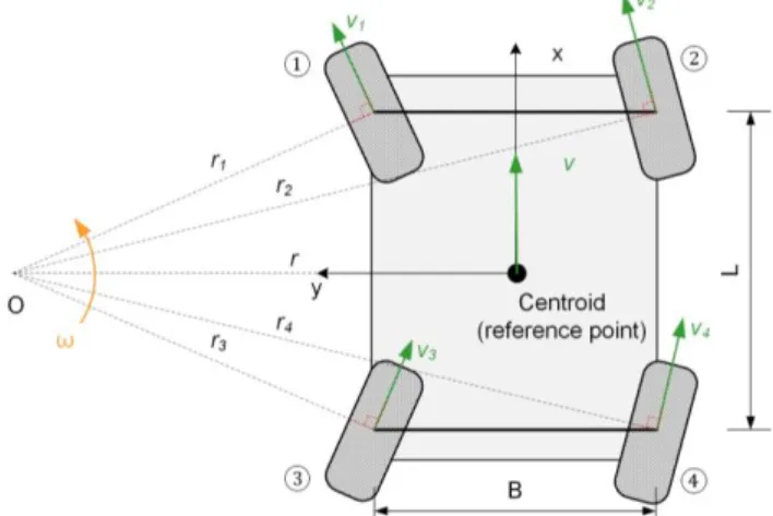
Fig. 1. Schematic diagram of a mobile robot model (planar) If the last of the above constraints is not active, the optimal solution is trivial and can be obtained using conventional methods based on “bang-bang” principle. In this case the desired motion is obtained by sequentially applying accelerations (amax, 0,amax) that produce either the trapezoidal or triangular velocity profile. However, generally, these constraints may compete to each other and the structure of the optimal solution becomes more complicated, which creates essential difficulties when generating time-optimal motion in real time. It should be mentioned that usually the constraint (9) is applied at the reference point of the mobile robot, which is the robot model centroid as shown in Fig. 1. However in practice, it is necessary to verify this constraint for each wheel, so the non-skidding constraint becomes slightly stronger. This particularity will be taken into account in the proposed motion generation algorithms.
3. REAL TIME MOTION GENERATION STRATEGY In classical control theory, the time-optimal motions for the second-order dynamic systems are generated using the conventional phase-plane method, taking into account specific properties of the optimal control input u t( ). It was proved that in the simplest case, when only the input constraint u amax is applied to the dynamic system (7), the optimal control has a “bang-bang” form, where the amplitude is constant u t( ) amax and there is a single switching from
max
u a to u amax. For the case where both limits
max
u a and s vmax are considered, the optimal control is also discontinuous, but it includes an intermediate interval with u t( )0 ensuring satisfaction of the velocity constraint. So, there are two switchings here, from u amax to u0
and from u0 to u amax. For these simple cases, the phase-plane method is efficient. But, as follows from relevant studies (Bobrow et al., 1985, Petrinić et al., 2017), application of the additional non-linear constraint similar to (9) can crucially change the structure of the optimal control function u t( ), which may include multiple switchings. To take into account approximately the non-linear constraint (9) and assume that at any time instant the time-optimal control operates at the limit of either the control input u or the admissible velocity s, let us present the modification of the classical phase-plane method. A basis idea here is to replace the primary upper bounds on the velocity and acceleration (8) by new values depending on the current state of the dynamic system( , )s s . Such way of combination of the inequalities (8) and (9) yields the modified bounds of the control input u and the velocity s:
2 2 2 max max 0 max max 0 ˆ min , ( ) ˆ min , ( ) a a u s r s v v u r s (10)that are included in the time-optimal motion planning algorithm. It is worth of mentioning that this modified phase-plane technique works perfectly well if the non-linear constraint (10) is not too hard, and it is satisfied even for the trajectory segments corresponding to u0. However, in the general case, the constraints (8) and (9) may compete strongly and the obtained forward and backward trajectories are not feasible (Gao et al., 2019).
An alternative approach to the time-optimal motion generation, which is proposed in (Gao, 2018), is based on the discrete dynamic programming. Because of its universal nature, this technique is able to take into account all considered constraints in a similar way and to generate optimal trajectories of complex structure that include multiple segments separated by so-called switching points (also known as discontinuity points, tangent points and singular critical points (Timar et al., 2005)). In contrast to the phase-plane method, the dynamic programming considers a set of feasible trajectories at each time instant, from which the best one is selected at the final stage. However, as follows from
our study, this approach is rather time consuming while applied to the entire displacement to be implemented. For example, in the case of grid 630×100, the total computation time for the time-optimal trajectory generation in Matlab R2014b was about two minutes (Intel i5 2.67GHz). For this reason, a “moving-window” strategy combined with dynamic programming for the real time optimal motion generation is proposed in this paper. Similar to the technique presented in (Gao et al., 2019), this strategy is able to generate feasible solutions while taking into account all the constraints, but it is significantly faster.
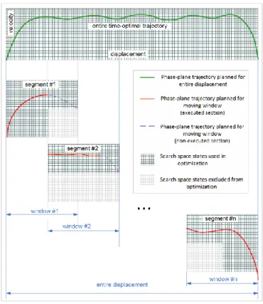
Fig. 2. Moving window scheme of real-time trajectory planning for mobile robot
This proposed approach breaks down the full-size problem into a set of sub-problems. As is shown in Fig. 2, a moving window is applied segment by segment. For each window, a developed trajectory planning algorithm (related information presented in next section) is used to generate the local time-optimal trajectory. The solution previously generated is already able to be implemented while the following computation is still ongoing. This allows implementing the feasible motion in real-time. In more details, an outline of the moving window scheme is presented below in the form of pseudo-codes. The input includes the arrays of displacement and path curvature { ( ), ( )S i R i i1, 2,... }n , velocity and acceleration limits, window size “width” and cut point “cutid”, as well as the discretization step of the velocity “dv”. The algorithm output is the optimal trajectory “VS”. The total procedure is composed of three basic steps. The first step defines the initial state, including the position, velocity and the distance to the end point. At the second step, a window with the desired size is applied starting from the second path point (since the starting point is known). A trajectory
Algorithm : real time motion generation
Input: Array of displacement – S(i), size 1×n
Array of radius – R(i), size 1×n
Maximum velocity / acceleration – vm / am Window entire width – width, integer number Executed segment width – cutid, integer number Velocity increment step – dv
Output: Optimal trajectory states – VS
Notations: Displacement to end point – d2e
Minimum distance for decelerating – ds Initial state – ini, size 1×3
Displacement for window – dis(i), size 1×width Radius for window – rs(i), size 1×width
Function: Motion planning for one window – DP_ planning
(1) Set d2e:= max(S); VS:= [0,0]; ini:= [VS, R(1)]; i:= 2; ds: = 0.5*vm*vm/am;
(2) While d2e>1.5*ds
Set dis: = S (i:width+i-1); rs: = R(i:width+i-1); [ vs ] = DP_ planning ( ini, dis, dv, rs, vm, am); VS : = [VS; vs(1:cutid)];
ini : = [vs(cutid), rs(cutid)]; d2e := d2e-(s(i+cutid -1)-s(i-1)); i:= i+cutid;
End
(3) Set dis := S(i:end); rs := R(i:end);
[ vs ] = DP_ planning ( ini, dis, dv, rs, vm, am); VS = [VS; vs];
planning function “DP_ planning” is invoked to generate the optimal solution for this window. Then, the generated trajectory is split into two parts at the “cutid” position. The former section is remained and the latter is removed. After that, the window is moved to the “cutid” position and the same operation is applied again. This process is repeated if the robot is not approaching to the final point. At the third step, the last window is applied to generate the trajectory ending with zero velocity at the final position.
4. MOTION PLANNING USING DISCRETE DYNAMIC RROGRAMMING FOR ONE SEGMENT
For one window (one segment), the motion generation problem is solved using discrete dynamic programming technique. To present the problem in a discrete way, let us sample the allowable domain of the velocity and displacement v[0,vmax] and s[0,smax] with the steps
v and s ( ) ( ) ; 0,1,... ; 0,1,... k i v k v k m s i s i n (11)
where v vmax m and s smax n. Then, for each path point we can generate a number of the mobile robot states with all possible velocities, i.e.siC( , )k i (v( )k ,s( )i);k. While considering the path points are ordered in time, the original sequence of sidescribed by presented equations may be converted into a directed graph presented in Fig. 3. It
should be noted that some of the states generated by previous equation should be excluded from the graph. These inadmissible states are not connected to any neighbor. It is clear that due to time-irreversibility, the allowable connections between the graph nodes are limited to the subsequent configuration states
1
(k ii, ) (ki,i1)
C C , and the edge weights correspond to the minimum travelling time.
Fig. 3. Graph-based presentation of the discrete search space for real-time trajectory planning
Using the discrete search space, the considered problem can be transformed to the searching of the shortest path on the above presented graph. In the frame of this notation, the desired solution can be represented as the sequence
2 1 (0,1) ( , 2) ( , 1) (0, ) { } { } ...{ } { } n k k n n C C C C . The distance between subsequent nodes can be evaluated as the displacement time in the following way:
1 1 ( , ) ( , 1) 1 ( , ) 2( ) ( ) i i i i k i k i i i k k dist s s v v C C (12)
The latter allows us to present the objective function (travelling time) as follows
1 1 ( , ) ( , 1) 1 ( , ) i i n k i k i i T dist
C C (13)that depends on the indices k k1, 2,...kn1,kn. It should be noted that the applied method of search space discretization automatically takes into account the velocity constraints, but the acceleration constraints must be examined as follows
1 max (vi vi) t a (14) where 1 ( , ) ( , 1) ( , ) i i k i k i t dist
C C . Additionally, the non-skidding condition (5) for each wheel should be also verified for computing the edge weights as follows
2 ( 2 )2
i i
a v R g (15) where can be estimated from (14).
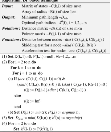
After discretization, the problem is converted to a combinatorial one, which can generally be transformed to the classical shortest path search on the graph. However, the straightforward approach is extremely more time-consuming than dynamic programming based technique (Gao, 2018). The developed algorithm breaks down the full-size problem into a set of sub-problems, aiming at finding the shortest path
Algorithm: DP based technique
Input: Matrix of states –C(k,i) of size m×n
Array of radius –R(i) of size 1×n
Output: Minimum path length –Dmin
Optimal path indices –k0(i), i = 1,2,…n
Notations: Distance matrix –D(k,i) of size m×n
Pointer matrix –P(j,i-1) of size m×n
Functions: Distance between nodes –dist ( C(k1,i1), C(k2,i2) )
Skidding test for a node –skid ( C(k,i), R(i) ) Acceleration test for nodes –acc (C(k1,i1), C(k2,i2))
(1) Set D(k,1):=0; P(k,1):=null; ∀k=1,2,…m (2) For i = 2 to n do
For k = 1 to m do For j = 1 to m do
(a) If (acc (C(k,i), C(j,i-1)) = 0) &
(skid ( C(k,i), R(i) )=0 ) & (skid ( C(j,i-1), R(i-1) )=0 ) r(j) := D(j,i-1)+dist ( C(k,i), C(j,i-1) )
else
r(j) := Inf end
(b) Set D(j,i) := min(r); P(j,i) := argmin(r); (3) Set Dmin := min( D(k,n) ); k0(n) := argmin(r)
(4) For i = 2 to n do
Set k0(i-1) := P(k0(i), i) from the initial
1 ( ,1) 1 {Ck ,k} to the current { ( , ), } i k i ki C . To present the basic idea, let us denote dk i, as the length of the shortest path connecting the initial node to the current node
( , )
{Ck i }. Then, taking into account the additivity of the objective (13), the shortest path for the nodes belong to the next layer {C( ,k i1),k} can be found by combining the optimal solutions for the previous layer {C(k i, ),k} and the distances between the nodes with the indices i and i1. The latter corresponds to the formula
, 1 min , ( ( , ), ( , 1))
k i k k i k i k i
d d dist C C (16)
that is applied sequentially starting from the second layer, i.e.
1, 2,... 1
i n . Finally, after selection of the minimum length
, 1
k i
d corresponding to the final layer and applying the
backtracking, one can get the desired optimal path in graph. It is described by the recorded indices { ,k k1 2,...kn1,kn}.
In more details, an outline of the developed algorithm is presented as follows in the form of pseudo-codes. The input includes the state matrix { ( , )C k i k1, 2,... ;m i1, 2,... }n
containing the information of displacement and velocity, and also the array of path radius { ( )R i i1, 2,... }n . The algorithm operates with two tables D k i( , ) and P k i( , ) that include the minimum distances for the sub-problem of lower size (for the path 1i) and the pointers to the previous locations respectively. The procedure is composed of four basic steps. The first step initializes the distance and pointer matrices. In step (2), the recursive formula (16) is implemented. The computing start from the second layer and it tries all possible connections between the nodes in the
current layer and the previous one. It includes verifications of the non-skidding constraint and acceleration limit in the sub-step (2a). The sub-sub-step (2b) finds the minimum path from the current node C k i( , ) to the first layer { ( ,1),C j j} and records the reference to { ( ,C j i 1), j} in the pointer matrix. In steps (3) and (4), the optimal solution is finally obtained and corresponding path is extracted by backtracking.
5. AN APPLICATION EXAMPLE
To evaluate the efficiency of the proposed technique, let us apply it to the generation of time-optimal motions along a sinusoidal path whose curvature varies essentially. This path is presented in Fig. 4 and is described by the parametric equations x A and y B sin( ) where [0, 4 ] and A B 10. The parameters of the mobile robot included in the constraints (8) and (9) are assumed to be as follows:
max 10.0 m s
v , 2
max 8.0 m s
a ,
0.9 and g9.8m s2.For this path of length smax152.72 m, the radius of curvature varies essentially from +10.00 m to the positive infinity and from the negative infinity to -10.00 m, which makes the non-skidding constraint (9) active at the path segments closest to the peak and the bottom.
Fig. 4. A sinusoidal path shape used for motion generation For this case study, the width of the window was about 15 m, which is higher than the minimum accelerating/decelerating distance 6.25 m. The displacement step s 0.28m and the velocity step v 0.10 m s. So, the search space of the first window was discretized with the grid 60×100. The computing time for the first window in Matlab R2014b was around 2.1 sec (Intel i5 2.67GHz). Then, all the next windows started from the 50th point of the previous one, and the sampling of v[0, 10] was replaced byv[5, 10]. So, with the reduced grid 60×50, the computing time for the following windows is less than 1.0 sec. In total, the computation time for the entire displacement was about 18.0 sec. It is much more efficient compared to the computational effort of our previous technique (more than 2 min). In order to meet the requirement of real time, this Matlab code was also transformed into the C code. In the environment of C, the computing time for entire displacement was 0.51 sec and for one window was 0.13 sec.
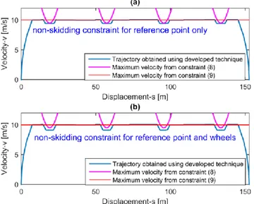
The obtained time-optimal trajectory is presented in Fig. 5, which shows that the desired motion is composed of multiple acceleration/deceleration segments separated by the relevant number of the switchings, which separate segments with
different active constraints. This result is in good agreement with physical nature of the problem, which requires reducing the speed in advance when closing to the path segments with high curvature to ensure pure rolling of the robot wheels. Hence, the proposed method allows user obtaining optimal trajectories in real time for any combination of linear/non-linear constraints describing limitations of the robot driving motors without skidding.
Fig. 5. Time optimal motion generated for sinusoidal path using moving window and discrete dynamic programming: (a) non-skidding constraint for reference point only; (b) non-skidding constraint for reference point and wheels.
6. CONCLUSIONS
Recent advances in mobile robotics and increase of their achievable driving speeds require essential improvement of existing motion generation algorithms. For this reason, in addition to the conventional velocity and acceleration constraints issued from the limited capacity of the driving motors, the “non-skidding” constraints imposed by the physical properties of the wheels contacts with the moving surface must be also considered. Because of the complicated description, they can be hardly integrated into existing motion planning algorithms that rely on the phase-plane method. To overcome this difficulty, the paper proposes a new technique that allows finding time-optimal motions along a curved path that takes into account limitations of the driving motors and also ensures the robot wheels rolling without skidding. After the state space discretization, the original problem is presented as a combinatorial one, where the desired robot trajectory is the shortest path on the relevant graph. To obtain this path and ensure its implementation in real time, a moving window strategy combined with dynamic programming is proposed. This technique allows taking into account all considered constraints in a similar way and generating optimal trajectories of complex structure that include multiple segments separated by switching points. Advantages of this technique and its suitability to real time control were confirmed by a case study dealing the fastest motion of the mobile robot along a sinusoidal path.
REFERENCES
Bharathi, A. & Dong, J. (2016). Feedrate optimization for smooth minimum-time trajectory generation with higher order constraints. The International Journal of Advanced
Manufacturing Technology, 82, 1029-1040.
Bobrow, J. E., Dubowsky, S. & Gibson, J. (1985). Time-optimal control of robotic manipulators along specified paths. The international journal of robotics research, 4, 3-17.
Butler, S. D., Moll, M. & Kavraki, L. E. (2016). A general algorithm for time-optimal trajectory generation subject to minimum and maximum constraints. Workshop on the Algorithmic Foundations of Robotics, 2016. Gao, J. (2018). Optimal motion planning in redundant
robotic systems for automated composite lay-up process.
École centrale de Nantes.
Gao, J., Pashkevich, A., Claveau, F. & Chevrel, P. (2019). Optimal motion generation for mobile robot with non-skidding constraints. IEEE 2019 International
Conference on Mechatronics. In press.
González, D., Pérez, J., Milanés, V. & Nashashibi, F. (2016). A review of motion planning techniques for automated vehicles. IEEE Transactions on Intelligent
Transportation Systems, 17, 1135-1145.
Jacobs, P. & Canny, J. (1993). Planning smooth paths for mobile robots. Nonholonomic Motion Planning. Springer.
Petrinić, T., Brezak, M. & Petrović, I. (2017). Time-optimal velocity planning along predefined path for static formations of mobile robots. International Journal of
Control, Automation and Systems, 15, 293-302.
Pfeiffer, F. & Johanni, R. (1987). A concept for manipulator trajectory planning. IEEE Journal on Robotics and
Automation, 3, 115-123.
Shiller, Z. & Lu, H.-H. (1992). Computation of path constrained time optimal motions with dynamic
singularities. Journal of dynamic systems, measurement,
and control, 114, 34-40.
Soueres, P. & Laumond, J.-P. (1996). Shortest paths synthesis for a car-like robot. IEEE Transactions on
Automatic Control, 41, 672-688.
Timar, S. D., Farouki, R. T., Smith, T. S. & Boyadjieff, C. L. (2005). Algorithms for time–optimal control of CNC machines along curved tool paths. Robotics and
Computer-Integrated Manufacturing, 21, 37-53.
Weiguo, W., Huitang, C. & Peng-yung, W. (1999). Optimal motion planning for a wheeled mobile robot. Robotics and Automation, 1999. Proceedings. 1999 IEEE International Conference on, 1999. IEEE, 41-46. Yang, H. S. & Slotine, J.-J. E. (1994). Fast Algorithms for
Near-Minimum-Time Control of Robot Manipulators: Communication. The International journal of robotics