Date of publication xxxx 00, 0000, date of current version xxxx 00, 0000. Digital Object Identifier 10.1109/ACCESS.2017.Doi Number
Frequency Response Analysis Interpretation
using Numerical Indices and Machine Learning:
A Case Study based on a Laboratory Model
Regelii S. de A. Ferreira1, Student member, IEEE, Patrick Picher2, Hassan Ezzaidi1, Member,
IEEE and Issouf Fofana1, Senior member, IEEE
1Research Chair on the Aging of Power Network Infrastructure (ViAHT), Université du Québec à Chicoutimi, Saguenay, QC, Canada 2Institut de recherche d’Hydro-Québec (IREQ), Varennes, QC, Canada
Corresponding author: Regelii S. de A. Ferreira (e-mail: [email protected]).
This work was supported by InnovÉÉ under Grant R11-1707 and by the Natural Sciences and Engineering Research Council of Canada (NSERC) under Grant RGPIN-2015-04403.
ABSTRACT Frequency response analysis is a powerful tool for mechanical fault diagnostics in power transformers. However, interpretation schemes still today depend on expert analyses, mainly because of the complex structure of power transformers. One of the fundamental shortcomings of experimental investigations is that mechanical deformations cannot be managed on real transformers to obtain data for different scenarios because they are too destructive. To address this issue in a systematic way, the current research used a specially designed laboratory transformer model that allows mechanical defects to be introduced so its frequency response can be evaluated under different conditions. The key feature of this model is the non-destructive interchangeability of its winding sections, allowing reproducibility and repeatability of frequency response measurements. Numerical indices were compared over key performance indicators (linearity, sensitivity and monotonicity). The analysis indicated that comparative standard deviation offered promising results for evaluation of mechanical deformations on the laboratory winding model given its monotonic behaviour, sensitivity and linear increase with fault severity. Additionally, support vector machine learning, radial basis function neural network and the statistical k-nearest neighbour method were used for fault classification with different strategies and configurations. While limited data from different transformers are used in the available literature, the approach discussed here considers 371 measurements from the same transformer model. The test results are supportive and demonstrate great accuracy when machine learning is used for winding fault classification.
INDEX TERMS Condition monitoring, frequency response analysis interpretation, machine learning, numerical indices, power transformers, radial basis function, support vector machines.
I. INTRODUCTION
Power transformers are essential assets of electrical power networks, and monitoring their operating condition is crucial for functional and economic reasons. Regular monitoring to ensure incipient failure is detected at the earliest stage is vital. Power transformers are vulnerable to through faults, which can result in significant mechanical forces on the active parts. In addition, insulation degradation due to ageing may cause a reduction in clamping pressure, increasing the risk of mechanical damage [1, 2]. Mechanical forces beyond the design limits of the transformer may cause deformations in the windings. Once such deformations occur, the transformer’s ability to withstand further mechanical forces
originating in a potential overcurrent is greatly reduced due to localized electromagnetic stresses [3].
Nowadays, there are many non-intrusive monitoring and diagnostic techniques available to detect incipient power transformer failures. These techniques evaluate the effects of different faults and can be implemented without requiring transformer disassembly. Frequency response analysis (FRA) is one of these methods, and it is currently commonly used in the electrical industry for condition assessment of transformer windings. From the very first studies [4], FRA has demonstrated its sensitivity for detecting mechanical and electrical failure modes [1, 5].
FRA compares current and reference frequency response measurements of a power transformer. Ideally, the reference measurements are obtained just before transformer energization, and subsequent monitoring over the years provides a continuous evaluation of the condition of the windings. Whenever reference traces are unavailable, traces from sister units (identical transformers) or other phases of the same transformer (in the case of three-phase transformers) can also be used. Deviations between current and reference measurements can indicate electrical or mechanical damage to transformer active parts.
Though FRA measurement procedures have been thoroughly studied at the international level in working groups of the IEEE [6], CIGRE [1] and the IEC [7], result interpretation still depends on expert analyses. Some of the quantitative interpretation methods proposed so far fall into three groups: numerical indices, white box physical models and artificial intelligence algorithms [8].
The frequency response of a transformer depends to a large extent on the type of transformer and its power rating, voltage rating, phase connections, winding design, etc. This means basic and fundamental principles using simple geometrical models, to guide the quantitative analyses.
This paper explores different measurements taken on a laboratory transformer model to study FRA interpretation. The model allows different deformations to be introduced and their influence on frequency response can then be evaluated. Four different fault modes (the fault extent varying) were introduced to the winding model: axial displacement (AD), radial deformation (RD), disc space variation (DSV) and short-circuited turns (ST). Numerical indices were then computed for quantitative interpretation of the different arrangements. The research also considered different frequency bands for application of the numerical indices, evaluating the sensitivity of the frequency range for numerical index calculations.
Machine learning classifiers were also compared over different architectures for an improved and objective fault classification. The classifiers use index calculation at target frequency bands as input for diagnosis of winding faults. Three main diagnostic categories were investigated: detection of fault occurrence; determination of fault type; determination of the fault type and extent
.
II. FREQUENCY RESPONSE ANALYSIS
FRA is a powerful tool for detecting mechanical changes in the active part of a power transformer. Since a transformer can be considered a complex network of RLC components [9] (resistance of the winding, inductance of the coils and capacitance of insulation layers and to the ground), variation in frequency response may indicate a physical change inside the transformer.
A frequency response is obtained by injecting a sinusoidal waveform at the reference point and measuring the amplitude and phase shift at the response point [1]. FRA traces can be
represented in terms of amplitude (HdB) (dB) and phase shift (φ) (degrees), as shown in (1) and (2)
HdB=20∙ log10(Vm/Vr) (1) φ=φ(Vm)-φ(Vr) (2) where, Vm is the response voltage and Vr is the reference voltage [1]. Amplitude (HdB) is widely used for interpretation purposes and numerical indices calculations.
There are also multiple measurement types depending on where the reference and response points are connected. The measurement types can be separated into two main groups: end-to-end measurements and interwinding measurements. End-to-end measurements are obtained when the signal is applied to one end of the winding and the response is measured at the other end of that same winding. Interwinding measurements are obtained when the signal is applied to one winding and the response is measured at another. The frequency response traces discussed in this paper were produced by an end-to-end open circuit measurement configuration and in some cases by an end-to-end short-circuit measurement, as described in [6].
The challenge when utilizing FRA to diagnose transformer active parts is mainly in the correct interpretation of deviations from current and reference measurements. Studies investigating FRA interpretation use numerical indices [10, 11], white-box modeling [12, 13] and artificial intelligence algorithms [14-17] to objectively assess frequency response traces obtained from real cases [8, 18], laboratory experiments [19] and simulation studies [20-22]. Different approaches for the interpretation of FRA measurements are reported in recent literature on the application of intelligent classifiers. For instance, the combination of numerical indices and intelligent classifiers is explored in [16, 23-26]. References [16, 23] use numerical indices as input to neural networks and discuss the use of support vector machine (SVM) for fault type recognition in power transformers. Reference [24] presents a method for locating shorted turns with FRA interpretation again based on numerical indices and SVM. However, the databases on which most of the studies reported in the literature are based are limited and the transformers types diverse.
The components of a transformer (tank, core, winding type, insulation type and so forth) also have an impact on its frequency response. Accordingly, the effects of transformer structures are explored in the literature [8, 21]. Reference [22] examines the identification of winding type by SVM. Transformer insulation plays a major role in frequency response, with liquid insulation changing the permittivity of the material, increasing capacitances and, as a result, shifting resonances to lower frequencies [27]. Meanwhile the migration of moisture into solid insulation has been reported to shift resonances to higher frequencies [28].
Nonetheless, the most common method of frequency response interpretation remains the visual comparison of reference and faulty traces. Numerical indices are applied to obtain a better quantitative interpretation. In the approach
proposed in this paper, frequency bands of interest (those where measurements deviate) were determined by visual inspection of the traces, and numerical indices were evaluated over these frequency bands. The frequency bands of interest and the best-performing numerical index were subsequently used as machine-learning input to achieve an objective interpretation of fault modes in FRA measurements.
A. FRA INTERPRETATION BASED ON NUMERICAL INDICES
Frequency response interpretation based on numerical indices is used to quantify differences between investigated and reference traces. Different indices [5, 10] evaluated over key performance indicators (such as linearity, monotonicity and sensitivity [29]) are suggested in the literature.
This research used some of the most promising numerical indices to evaluate frequency response measurements [8]. A description of these indices is presented in Table 1.
TABLEI
SUMMARY OF NUMERICAL INDICES USED IN THIS RESEARCH
Index Description Equation
CCF The cross-correlation factor quantifies the linear dependence between two data sets. Its value is closer to 1 if there is large positive correlation between the data sets and closer to zero in case of a weak correlation.
(3)
LCC Lin’s concordance coefficient measures the agreement between two variables. A value near 1 indicates a strong concordance, a value close to zero denotes a weak concordance, and a value near -1 denotes strong discordance.
(4)
CSD Comparative standard deviation is zero in case of a complete match of traces, and there is no upper limit value. For amplitude deviations, this index has lower sensitivity [8, 30].
(5)
SSE The sum squared error calculates the square of the distance between two traces. A value close to zero means a good match of traces, and there is no upper limit value. The index has shown low sensitivity for amplitude deviations [8], though its sensitivity is improved when amplitude deviations occur around resonance points [11].
(6)
SSRE The sum squared ratio error uses the squared ratio error between two traces. A value of zero indicates a good match of data, and there is no upper limit value. Like other squared sums, this index presents less linear behaviour [8].
(7)
The numerical indices described in Table 1 and used in this paper are calculated in equations (3) to (7), where, X and Y are the magnitude vectors of reference and investigated frequency responses respectively, X(i) and Y(i) are the ith element of these vectors and N is the number of data points
CCF= ∑ (X(i)-X̅)(Y(i)-Y̅)
N i=1
√∑N (X(i)-X̅)2
i=1 ∑Ni=1(Y(i)-Y̅)2
(3)
LCC=
2
N∑ (X(i)-XNi=1 ̅)(Y(i)-Y̅)
(Y̅-X̅)2+1
N∑ (X(i)-XNi=1 ̅)2+N1∑ (Y(i)-YNi=1 ̅)2
(4) CSD=√∑ [(X(i)-X̅) -(Y(i)-Y̅)]2 N I=1 N-1 (5) SSE=∑ (Y(i)-X(i)) 2 N i=1 N (6) SSRE= ∑ (Y(i)X(i)-1) 2 N i=1 N (7)
where, X̅=1/N ∑ X(i)Ni=1 and Y̅=1/N ∑ Y(i)N
i=1 .
Not only must the numerical index that will be used to evaluate the frequency response traces be selected, but the frequency band to which this index is applied must be determined as well, and this can be challenging. Different methods can be used, the simplest being to evaluate the entire frequency range in the same way, as described in [31, 32]. This approach, however, can result in a lack of sensitivity to deviations in a small range of the frequency response. Division of the frequency range into sub-ranges is, accordingly, usually explored [7, 33]. To achieve an independent frequency range subdivision, the study described in [29] suggests a frequency window that sweeps the total frequency range, evaluating some of the traces at each window step.
B. FRA INTERPRETATION BASED ON MACHINE LEARNING
Machine learning and neural networks are intelligent algorithms frequently used to classify patterns by learning from examples. Given their adaptive characteristic, these classifiers have been widely used for fault diagnostics in power transformers [16, 23, 34].
Two approaches are used for network learning by example: unsupervised and supervised learning. With unsupervised learning, there is no need to supervise the network and provide target outputs to match inputs. With supervised learning, the network is provided with a target output for each input vector injected. Based on the computed output error (difference between the target output and the estimated output), the network adjusts its synaptic weights using heuristic algorithms at each iteration.
This paper compares several well-known and widely used machine learning classifiers: radial basis function (RBF) neural network, support vector machine (SVM) and the statistical k-nearest neighbour (k-NN). These models have become very popular in recent years because of their ability to solve problems in classification, regression and other applications in different areas.
1) RADIAL BASIS FUNCTION
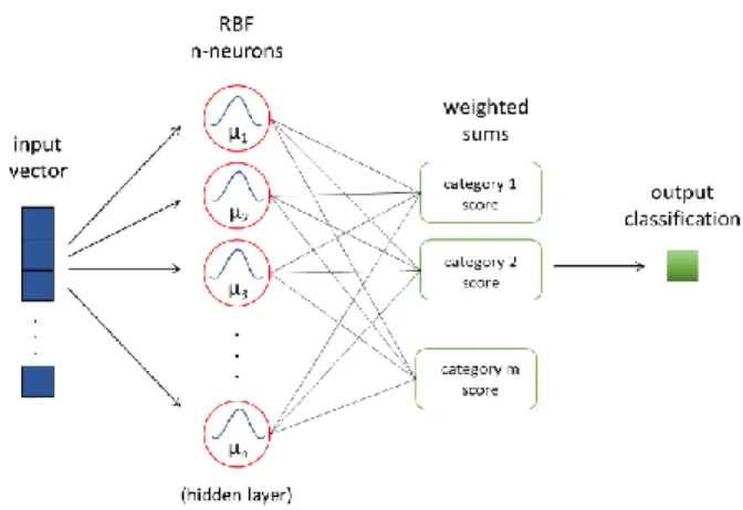
RBFs are feed-forward multilayer structures. The output node is a decision based on a linear combination of the RBF outputs computed by the hidden layer neurons. Each RBF neuron stores a prototype information vector and then compares the input vector to its prototype. The output of each neuron is a value between zero and 1, which is a similarity measure. If the input is equal to the prototype, then the output of that neuron will be 1. The response tends to zero as the difference between the input and the prototype increases. The shape of the RBF neuron’s response is a bell curve, as illustrated in the network architecture diagram in Fig. 1.
FIGURE 1. Radial basis function neural network architecture.
2) SUPPORT VECTOR MACHINE
The SVM is a supervised learning model with associated learning algorithms. Even though SVMs were first applied to binary class problems, they can also be applied to multiclass problems by using one-versus-one and one-versus-all heuristic methods to split and transpose the multiclass into a binary classification problem. The SVM model is considered a generalization of linear classifiers when classifying a set of linearly separable patterns (xi) from two classes: C1 and C2. This is achieved by positioning an appropriate hyperplane as a decision boundary satisfying the equation g(x)=wtx +b=0, where w is the weight vector and b is the bias or threshold. All pattern data xi with g(xi)>0 are assigned to C1 and those with g(xi)<0 are assigned to C2. However, SVMs choose the linear separator with the largest margin, centered between two hyperplanes described by equations (8) and (9):
h1(xi)=wtxi+b ≥1, for xi ∈ C1 (8) h2(xi)=wtxi+b ≤-1, for xi ∈ C2 (9) The distance between the hyperplanes h1 and h2 is the margin, and all points that lie on h1 or h2 are called support vectors. To take into account the non-separable data xi, a slack variable ξi is incorporated to give more relaxation at the constraints, yielding a compact form of the previous equations as follow:
yi(wtx
i+b) ≥1-ξi, for i=1, 2, …N, (10) with yi=1 if xi ∈ C1 and yi=-1 if xi ∈ C2.
The margin to be maximized is then equal to 1/‖w‖, and the primal formulation of the SVM task is to find the optimal weights and bias that will minimize the cost function defined in (11) φ(w,b,ξ)=1 2w tw+ρ ∑ ξ i N i=1 , (11)
while satisfying the constraints in (10), with ξi≥0 for i=1, 2, …N. The parameter ρ, referred to as the regularization parameter, controls the penalty of non-separable points.
Using the method of Lagrange multipliers and formulating the optimization problem from a dual problem perspective, the objective function (12) to be maximized is obtained [35].
Q(α)= ∑ 𝛼𝑖 𝑁 𝑖=1 -1 2∑ ∑ yiyjαiαjxiTxj N j=1 N i=1 . (12)
The equation (12) is subjected to the constraints ∑Ni=1yiαi=0 and 0≤αi≤ρ for all i, where αi is a set of Lagrange multipliers.
The SVM algorithms use a set of mathematical functions that are defined as kernel functions. In SVM models, kernel functions are used to transform the non-linear space into a higher dimensional linear space, changing the objective function as follows: Q(α)= ∑ αi N i=1 -1 2∑ ∑ yiyjαiαjkernel(xi,xj) N j=1 N i=1 . (13)
The software used to train the SVM model is based on the iterative single data algorithm (ISDA) solver [36]. The cost ρ applied to the misclassification in training data is defined as 1. The regularization parameter for smoothing is fixed at 1/N, where N is the number of observations. Each class is then centred by its mean value and scaled by its standard deviation. Before evaluation of the kernel(xj,xk), where xjand xk are the training datasets, an appropriate factor is selected automatically by the software to scale the data and 0.1 is added as kernel offset.
For this research, three popular kernel functions were considered: linear, Gaussian and polynomial. A one-versus-one heuristic method (or coding design) and a one-versus-one-versus-all method were tested for SVM classification algorithms. The kernel functions were investigated and compared using default SVM methods. The functions explored in this paper are shown in equations (14) to (16). The linear kernel function is defined as:
G(xj,xk)=xj'xk, (14) the polynomial kernel function with order p=3, is defined as:
G(xj,xk)=(1-xj'xk) p
, (15)
the Gaussian kernel function is defined as:
G(xj,xk)=e (−‖xj-xk‖
2 σ2 )
, (16)
where the standard deviation (σ) is set to 1. 3) K-NEAREST NEIGHBOUR
In machine learning, k-NN is a non-parametric algorithm used for classification and regression. Based on similarity measures, the k-NN algorithm assigns the test pattern in the category to the class which has the majority of nearest neighbours. Though k-NN is considered the simplest algorithm, in practice the learning vector quantization (LVQ) algorithm seems more appropriate and simpler. LVQ is based on a reduced number of prototypes that can be estimated using the k-means algorithm. LVQ classification is based on the similarity measure of the test pattern and the prototypes representing each category.
The k-NN function is only approximated locally, and the only parameter of the algorithm is the number of neighbours (k) considered for classification, where k is a positive integer. If k=1, the input is assigned to the class of that single nearest neighbour. For the best algorithm performance, a normalization of the database is often required. A data set with different physical units or different scales can seriously undermine the accuracy of the algorithm [37].
III. LABORATORY WINDING MODEL AND REFERENCE MEASUREMENTS
Measurements were taken from 1 kHz to 1 MHz on a laboratory winding model with removable sections using a commercially available FRA instrument. The model was designed and manufactured to enable short-circuits and different mechanical deformations [19].
The laboratory winding model used for this study is of uniform structure, that is, same conductor throughout the winding and an equal number of turns per winding section. The model has solid, non-grated insulation and was designed specifically for FRA testing: that is, there are no power or voltage ratings for the model.
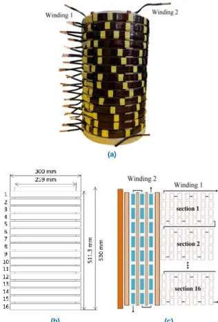
Fig. 2 shows the model and its connection schematic. The transformer model is composed of two windings, the outer coil (winding 1) with 448 turns divided into 16 sections (28 turns per section) and the inner coil (winding 2) divided into three concentric and fixed layers with 76 turns each, a total of 228 turns in this winding.
The inner diameter of winding 1 is 300 mm, its radial dimension is 8.5 mm and its height is 511.3 mm. Winding 2 has an inner diameter of 259 mm, a radial dimension of 9 mm and a total height of 530 mm. The outer winding of the transformer model has 16 sections. These sections facilitate defect introduction at different locations.
All FRA measurements discussed in this paper were taken with an air core and concentrically arranged coils, as shown in Fig. 2. The reference measurements (healthy winding) for windings 1 and 2 are presented in Fig. 3. The curves in Fig. 3 serve as reference for comparison with fault modes.
As Fig. 3 shows, the first anti-resonance for the open circuit measurement appears at a frequency around 25 kHz for both windings. A magnetic core, not present in this laboratory model, would create a high-magnetizing inductance and a first anti-resonance frequency below 1 kHz. The short-circuit
measurement matches the open circuit measurement at over 150 kHz, in both windings. Since the faults were introduced on winding 1, the open-circuit measurement taken from winding 1 was used in this research to compare faulty and healthy states.
(a)
(b) (c)
FIGURE 2. Model for laboratory tests: (a) winding photo, (b) dimensions and (c) connections schematic.
(a) (b)
IV. FAULT ANALYSES
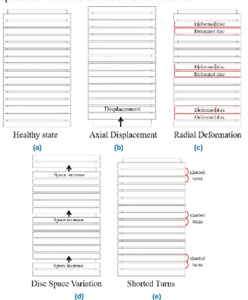
For this research, four different fault modes were introduced in winding 1: three mechanical deformations and one electrical fault. Six levels of each fault were tested to verify the evolution of the fault in the frequency response. Fig. 4 is a sketch representation of the fault modes.
A. AXIAL DISPLACEMENT
Axial displacement (AD) faults were created by adding spacers at the bottom of winding 1, resulting in vertical displacement between winding 1 and winding 2. The AD fault started with 6 mm spacer (AD 1) and increased the spacers in steps of approximately 5.4 mm up to 34 mm (AD 6). Fig. 5.a shows the frequency response for reference and the AD fault steps.
B. RADIAL DEFORMATION
Radial deformation (RD) faults were created by replacing healthy sections of winding 1 by deformed ones. The model has sixteen identical healthy sections. Six radially deformed sections were used to replace healthy sections and introduce radial deformation to the model. The RD fault started by replacing one healthy section with a deformed one, and then replaced one more for each fault step in the positions indicated in Fig. 4.c., such that RD 1 has one deformed section and RD 6 has six. Fig. 5.b shows the frequency response for reference and RD faults.
C. DISC SPACE VARIATION
Disc space variation (DSV) faults were created like the AD faults, but the spacers were added between sections at three different positions, as shown in Fig. 4.d. The first DSV fault level (DSV 1) has 6 mm spacer between sections 2 and 3. DSV 2 has 11.4 mm spacer between the same sections. The next DSV fault steps were created by adding first 6 mm and then 11.4 mm spacers between sections 8 and 9. The last two steps were created by adding 6 mm (DSV 5) and then 11.4 mm (DSV 6) spacers between sections 14 and 15. Spacers were always added without removing those for the previous levels, increasing the fault extent at each step. Fig. 5.c shows the frequency response for reference and DSV faults.
D. SHORT-CIRCUITED TURNS
The final fault, the shorted turns (ST) fault, is an electrical fault created by generating a short-circuit between turns of winding 1. The ST fault started with a short-circuit of section 2 of winding 1 (ST 1), for a total of 28 turns shorted. For ST 2 the turns of sections 2 and 3 were shorted, for a total of 56 turns shorted. Shorted turns continued to be added to
winding 1 until sections 2, 3, 8, 9, 14 and 15 (ST 6) were all shorted, for a total of 168 turns shorted. At each level, the shorted sections were added without correcting those of the previous levels, so the impact of shorted turns all along winding 1 could be observed. Fig. 5.d shows the frequency response for reference and the six ST fault levels.
(a) (b) (c)
(d) (e)
FIGURE 4. Winding model representation of fault modes: (a) healthy state; (b) axial displacement; (c) radial deformation; (d) disc space variation; and (e) shorted turns.
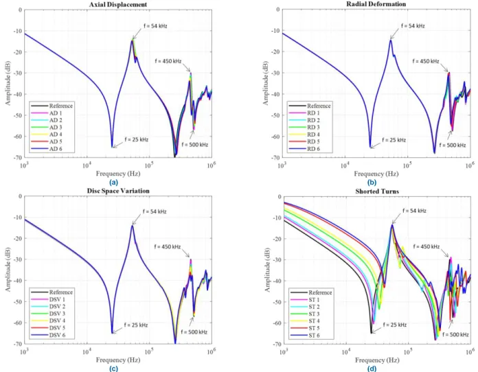
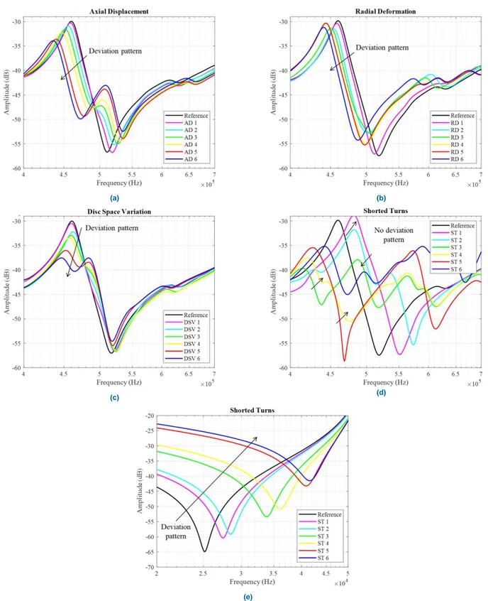
Fig. 5 shows frequency responses for the different faults analyzed in this study. As the figure demonstrates, the faults have different impacts on frequency response. The first resonance at 25 kHz was not affected by the mechanical deformations, but the shorted turns had a substantial effect in this region. This is mainly because the lower frequency region is dominated by the main inductance of the transformer and the ST fault reduces this inductance significantly. Reducing coil inductance results in frequency response displacement towards higher frequencies, as clearly shown in Fig. 6.e. The next anti-resonance point along the frequency response curve, at around 54 kHz, is less affected by the faults. In fact, this point is not even much affected by the ST fault, though the entire frequency range (1 kHz to 1 MHz) is greatly affected by this electrical fault.
(a) (b)
(c) (d)
FIGURE 5. FRA measurements for the different fault modes: (a) axial displacement; (b) radial deformation; (c) disc space variation; and (d) shorted turns.
The last frequency region of interest is 400 kHz to 700 kHz, where a resonance at 450 kHz and an anti-resonance at 500 kHz are present (these resonance frequencies are observed in the healthy winding). This particular frequency range (400 kHz to 700 kHz) was affected by all faults (mechanical and electrical), as shown in Fig. 6.
Each of the faults affected the frequency range from 400 kHz to 700 kHz differently. As a result, this frequency was used to calculate indices for quantitative evaluation of the faults. However, unlike the mechanical faults, the ST fault did not present a clear deviation pattern at this frequency band, as shown in Fig. 6. The frequency range from 20 kHz to 50 kHz was thus used to evaluate ST faults, since the deviation pattern is clearer in this region.
The curves in Fig. 7 show the numerical indices calculated from equations (3) to (7) for the different levels of fault in the frequency range from 400 kHz to 700 kHz for the mechanical faults and the range from 20 kHz to 50 kHz for the ST fault. Note that the indices CCF and LCC are evaluated as CCF*=1-CCF and LCC*=1-LCC to simplify comparison with other indices. Also, to facilitate indices comparison, a normalization was performed, each index value being divided
by the maximum value of its group to obtain a rescale between zero and 1.
All the indices evaluated presented monotonic behaviour for the different faults; that is, for higher levels of the fault, the indices presented their highest value. In addition, the indices all appeared to be linear, though some indices in general are not linear: for example, when the indices include squared calculations. The sensitivity of the indices was not consistent, especially at the lowest fault level, which most indices were unable to detect. The CSD index, however, showed good sensitivity, even at the lowest fault level, for all faults, with a value of at least 18% when comparing the first deformation step with the last step up in all cases. Furthermore, the CSD index showed the best overall results for this analysis given its monotonic, linearity and sensitivity behaviour.
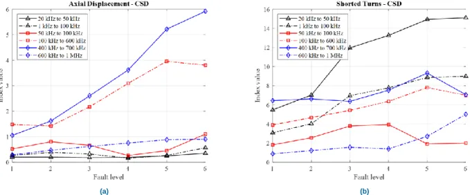
Fig. 8 shows an analysis of the frequency ranges used for the index calculations. Frequency ranges from the first resonance (20 kHz to 50 kHz), the first anti-resonance (50 kHz to 100 kHz) and the deviations in fault analysis (400 kHz to 700 kHz) are compared to the Chinese standard [33] frequency band divisions: 1 kHz to 100 kHz; 100 kHz to 600 kHz; and 600 kHz to 1 MHz.
(a) (b)
(c) (d)
(e)
FIGURE 6. Frequency response at a frequency range affected in fault mode: from 400 kHz to 700 kHz for (a) axial displacement, (b) radial deformation, (c) disc space variation and (d) shorted turns; and from 20 kHz to 50 kHz for (e) shorted turns.
(a) (b)
(c) (d)
FIGURE 7. Numerical index analyses for fault modes (a) axial displacement; (b) radial deformation; (c) disc space variation; and (d) shorted turns.
(a) (b)
To simplify this last comparison, only the AD and the ST faults were evaluated, the other mechanical faults demonstrating results similar to the AD fault. In addition, only the CSD index was used for this comparison, since it offered the best overall performance for fault evaluation in this laboratory winding model. The CSD index was not normalized for this comparison.
Fig. 8.a shows that the monotonic behaviour of the CSD index disappeared in most frequency ranges and linearity was observed only from 400 kHz to 700 kHz. This indicates that the frequency range analyzed has a substantial impact on index results and that the frequency bands suggested in [33] are not suitable for the winding model studied. In Fig. 8.b, on the other hand, monotonic behaviour appears in the frequency bands suggested by [33] but there is less linearity, mainly due to this fault’s characteristics, once again confirming the need for care in determining the frequency bands to be used for index calculation.
V. RECOGNITION PERFORMANCE AND DISCUSSION
Three machine learning classifiers were investigated in an effort to obtain a more objective interpretation for fault diagnostics in a winding model: radial basis function (RBF), support vector machine (SVM) and k-nearest neighbour (k-NN).
The measurements shown in Fig. 5 were replicated under very similar conditions, providing a large database of measurements. After disassembling and reassembling sections of winding 1, small deviations were noted in the winding frequency response, giving slight differences in index values. A total of 371 measurements (with and without faults) were taken. For the proposed classifiers, 80% of the measurements were used for training, leaving 20% for testing and validation.
The input vectors were composed of CSD index values in the three main frequency bands of interest (20 kHz to 50 kHz; 50 kHz to 100 kHz; and 400 kHz to 700 kHz).
Three types of fault identification were investigated. In the first scenario, the intelligent classifiers were trained and tested to issue a binary decision on the presence or absence of a fault regardless of fault type or nature. Since the learning was qualified as supervised, all fault data were assigned to class C1 and data without fault were assigned to class C2 (binary analysis).
Determination of fault type was introduced in the second scenario. The intelligent algorithms were asked to identify fault type (5 classes): no fault detected, AD, RD, DSV or ST. In the third and last scenario, the classifiers were requested to identify fault type (as above) along with fault extent (1 to 6). This calls for discrimination between 25 classes, considerably reducing the amount of data per class and possibly negatively affecting statistical convergence of the network.
The architecture of the suggested RBF neural network comprises an input layer, a hidden layer and an output layer.
The neurons in the hidden layer contain Gaussian activation functions whose outputs are inversely proportional to distance from the centre of the neuron. The neurons in the second layer contain a linear activation function (purelin) for categorization purposes. Both layers have biases. The smoothing parameter (spread) of radial basis functions was fixed at 1.
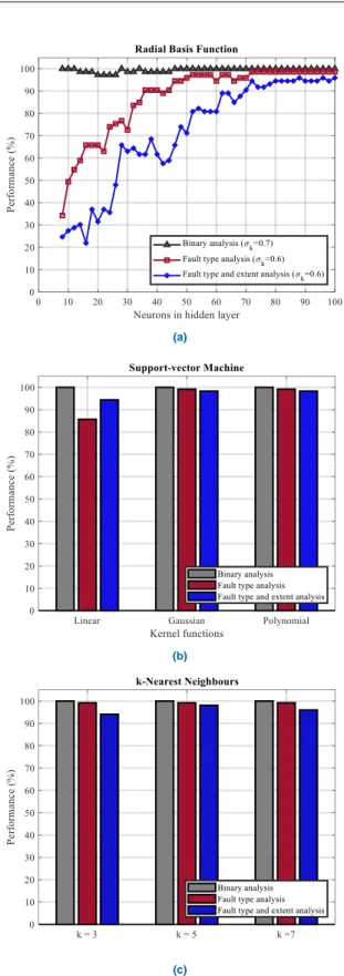
Figure 9 shows the results for the machine learning classifiers in all the suggested scenarios. The optimization problem in RBF neural network structures is to find the optimal number of hidden layer neurons and their corresponding spread σk and centroids μk. To find the best value for these parameters, several architectures were considered, trained and tested using 80% and 20% of the measurements, respectively, as described above. For each architecture, the number of neurons in the hidden layer was increased from eight to 100 neuron cells in increments of two. The impact of spread was also investigated, varying σk from 0.6 to 1 in increments of 0.1. In normal distributions, variation of the standard deviation impacts the spread of the distribution curve; higher standard deviations spread out the distribution, while lower ones mean a less spread distribution and a more pronounced peak.
As Fig. 9.a shows, the RBF neural network demonstrated high accuracy (above 98%) in the binary analysis (determining presence or absence of fault) even when using only 8 neurons in the hidden layer. For this analysis, the spread value of σk=0.7 showed the best performance, though results were very close for all spread values verified. The RBF network’s performance in determining fault type was good, more than 90% accurate when at least 40 neurons were used and more than 80% accurate when at least 32 neurons were used. For this analysis, the best performance was obtained with the spread value σk=0.6. When the RBF neural network was asked to determine fault type and extent, accuracy only exceeded 80% with at least 52 neurons; for 90% accuracy or more, it took at least 70 neurons— considered disproportionate given the size of the database. To overcome this problem, the amount of data available to train the network would have to be increased. For fault type and extent analysis, the best performance was obtained with spread value σk=0.6.
As Fig. 9.b shows, all SVM kernel functions performed well (accuracy > 85%) in the three analyses. The figure also indicates that the performance of the Gaussian and polynomial functions was very close. In fact, these functions are, overall, the best kernel function choice for analysis of the suggested data set, achieving 98% accuracy for fault type and extent detection. Meanwhile, SVM using Gaussian or polynomial kernel functions obtained above 99% accuracy in determining presence or absence of fault. Comparison of the one-versus-one and one-versus-all heuristic methods for SVM algorithms did not show significant variation in their results. To simplify the results, the one-versus-all heuristic method was selected for the graphic presentation.
(a)
(b)
(c)
FIGURE 9. Machine learning architecture performances: (a) radial basis function neural network; (b) support-vector machine; and (c) statistical k-nearest neighbour.
For the statistical model k-NN, the impact of the number of neighbours was evaluated, that is, k = 3, 5 and 7. The performance of this model was also above 94% for the three
classification models studied. These results are shown in Fig. 9.c.
The research described in this paper is a proof of concept study. The main advantage of the approach taken was the opportunity to investigate a large number of failure modes and different failure extents on the same unit, as compared to past studies that used limited databases and real transformers, which can be problematic to interpret. A three-phase transformer model that is closer to the real model is being developed so this research can continue in the near future. With this approach and the new model, it should be possible to obtain results that can be more closely generalized to real-case transformers.
VI. CONCLUSION
This paper reports on frequency response interpretation using numerical indices and machine learning applications. Used for the study was a specially designed laboratory transformer model that allows mechanical defects to be introduced so its frequency response under different circumstances can be evaluated. This model has removable sections and is designed and manufactured to enable short-circuits and deformations (axial and/or radial), allowing reproducibility and repeatability of frequency response measurements. Numerical indices were used to evaluate deviations derived from axial displacements, radial deformations, disc space variations and short-circuited turns integrated into the outer winding.
The results of the index evaluations showed that while all the indices were able to identify the highest levels of deformations in the frequency range of interest (400 kHz to 700 kHz), best overall results were obtained in this study with the CSD, given its monotonic behaviour, linear increase with fault severity and sensitivity even to the smallest deformations.
Results for use of machine learning classifiers for fault diagnostics were promising. The RBF, SVM and k-NN networks performed well classifying faults using the CSD index and targeted frequency bands as input. An automatic- interpretation for fault extent detection in addition to fault classification would be a major asset in power transformer condition monitoring. This remains one of the challenges of our research activities.
REFERENCES
[1] CIGRE Technical Brochure 342, "Mechanical-Condition Assessment of Transformer Windings Using Frequency Response Analysis (FRA)," 2008.
[2] A. Abu-Siada, N. Hashemnia, S. Islam, and M. Masoum, "Understanding power transformer frequency response analysis signatures," IEEE Electr. Insul. Mag., vol. 29, no. 3, pp. 48-56, 2013, DOI: 10.1109/MEI.2013.6507414.
[3] J. F. Araujo, E. G. Costa, F. L. M. Andrade, A. D. Germano, and T. V. Ferreira, "Methodology to Evaluate the Electromechanical Effects of Electromagnetic Forces on Conductive Materials in Transformer Windings Using the Von Mises and Fatigue Criteria," IEEE Trans.
Power Deliv., vol. 31, no. 5, pp. 2206-2214, 2016, DOI:
[4] E. P. Dick and C. C. Erven, "Transformer diagnostic testing by frequency response analysis," IEEE Trans. Power Appar. Syst., vol. PAS-97, no. 6, pp. 2144-2153, 1978, DOI: 10.1109/TPAS.1978.354718.
[5] P. Picher, S. Tenbohlen, M. Lachman, A. Scardazzi, and P. Patel, "Current state of transformer FRA interpretation: On behalf of CIGRE WG A2.53," in Procedia Eng., 2017, vol. 202, pp. 3-12, DOI: 10.1016/J.PROENG.2017.09.689. [Online].
[6] IEEE Std C57.149-2012, "IEEE Guide for the Application and Interpretation of Frequency Response Analysis for Oil-Immersed Transformers," 2013, DOI: 10.1109/IEEESTD.2013.6475950. [7] IEC 60076-18, "Measurement of frequency response," 2012. [8] CIGRE Technical Brochure 812, "Advances in the interpretation of
transformer Frequency Response Analysis (FRA)," 2020.
[9] M. F. Lachman, V. Fomichev, V. Rashkovsky, and A. Shaikh, "Frequency response analysis of transformers: visualizing physics behind the trace," Proc. 78th Annual Int. Conf. Doble Clients, Sec. T-14, 2011.
[10] M. H. Samimi, S. Tenbohlen, A. A. S. Akmal, and H. Mohseni, "Evaluation of numerical indices for the assessment of transformer frequency response," IET Gener. Transm. Distrib. vol. 11, no. 1, pp. 218-227, 2017, DOI: 10.1049/IET-GTD.2016.0879.
[11] M. H. Samimi and S. Tenbohlen, "FRA interpretation using numerical indices: State-of-the-art," Int. J. Electr. Power Energy Syst., Review vol. 89, pp. 115-125, 2017, DOI: 10.1016/J.IJEPES.2017.01.014. [12] N. Abeywickrama, Y. V. Serdyuk, and S. M. Gubanski,
"High-frequency modeling of power transformers for use in "High-frequency response analysis (FRA)," IEEE Trans. Power Deliv., vol. 23, no. 4, pp. 2042-2049, 2008, DOI: 10.1109/TPWRD.2008.917896. [13] S. Tenbohlen, M. Tahir, E. Rahimpour, B. Poulin, and S. Miyazaki,
"A new approach for high frequency modelling of disk windings," CIGRE, A2-214, 2018.
[14] S. w. Fei and X. b. Zhang, "Fault diagnosis of power transformer based on support vector machine with genetic algorithm," Expert Syst. Appl., vol. 36, no. 8, pp. 11352-11357, 2009, DOI: 10.1016/J.ESWA.2009.03.022.
[15] X. Mao, Z. Wang, P. Crossley, P. Jarman, A. Fieldsend-Roxborough, and G. Wilson, "Transformer winding type recognition based on FRA data and a support vector machine model," High Volt., vol. 5, no. 6, pp. 704-715, 2020, DOI: 10.1049/HVE.2019.0294.
[16] M. Bigdeli, P. Siano, and H. H. Alhelou, "Intelligent Classifiers in Distinguishing Transformer Faults Using Frequency Response Analysis," IEEE Access, vol. 9, pp. 13981-13991, 2021, DOI: 10.1109/ACCESS.2021.3052144.
[17] A. J. Ghanizadeh and G. B. Gharehpetian, "ANN and cross-correlation based features for discrimination between electrical and mechanical defects and their localization in transformer winding," IEEE Trans
Dielectr. Electr. Insul., vol. 21, no. 5, pp. 2374-2382, 2014, DOI:
10.1109/TDEI.2014.004364.
[18] R. S. A. Ferreira, H. Simard, P. Picher, V. Behjat, I. Fofana, and H. Ezzaidi, "Case study for assessing the integrity of a service-aged transformer repair using Frequency Response Analysis (FRA)," presented at the 2019 CIGRE Canada Conf., Montréal, Québec, 2019. [19] R. Youssouf, R. Ferreira, F. Meghnefi, H. Ezzaidi, I. Fofana, and P. Picher, "Frequency Response of Transformer Winding: A Case Study based on a Laboratory Model," in 2018 IEEE Conf. Elect. Insul.
Dielect. Phenom. (CEIDP), 2018: IEEE, pp. 271-274.
[20] Z. Wang, J. Li, and D. M. Sofian, "Interpretation of Transformer FRA Responses - Part I: Influence of Winding Structure," IEEE Trans.
Power Deliv., vol. 24, no. 2, pp. 703-710, 2009, DOI:
10.1109/TPWRD.2009.2014485.
[21] D. M. Sofian, Z. Wang, and J. Li, "Interpretation of Transformer FRA Responses - Part II: Influence of Transformer Structure," IEEE Trans.
Power Deliv., vol. 25, no. 4, pp. 2582-2589, 2010, DOI:
10.1109/TPWRD.2010.2050342.
[22] X. Mao, Z. Wang, P. Jarman and A. Fieldsend-Roxborough, "Winding Type Recognition through Supervised Machine Learning using Frequency Response Analysis (FRA) Data," 2019 2nd Int. Conf. Elect.
Materials Power Equip. (ICEMPE), Guangzhou, China, 2019, pp.
588-591, doi: 10.1109/ICEMPE.2019.8727354.
[23] M. Bigdeli, M. Vakilian, and E. Rahimpour, "Transformer winding faults classification based on transfer function analysis by support vector machine," IET Electr. Power Appl., vol. 6, no. 5, pp. 268-276, 2012, DOI: 10.1049/IET-EPA.2011.0232.
[24] A. Moradzadeh and K. Pourhossein, "Application of Support Vector Machines to Locate Minor Short Circuits in Transformer Windings,"
2019 54th Int. Univer. Power Eng. Conf. (UPEC), Bucharest,
Romania, 2019, pp. 1-6, doi: 10.1109/UPEC.2019.8893542. [25] V. Nurmanova, M. Bagheri, A. Zollanvari, K. Aliakhmet, Y.
Akhmetov and G. B. Gharehpetian, "A New Transformer FRA Measurement Technique to Reach Smart Interpretation for Inter-Disk Faults," in IEEE Trans.Power Deliv., vol. 34, no. 4, pp. 1508-1519, Aug. 2019, doi: 10.1109/TPWRD.2019.2909144.
[26] M. Bigdeli, D. Azizian, and G. B. Gharehpetian, ‘‘Detection of probability of occurrence, type and severity of faults in transformer using frequency response analysis based numerical indices,’’
Measurement, vol. 168, Jan. 2021, Art. no. 108322.
[27] P. Picher, C. Rajotte, and C. Tardif, "Experience with frequency response analysis (FRA) for the mechanical condition assessment of transformer windings," in 31st Elect. Insul. Conf. EIC, Ottawa, Canada, 2013, pp. 220-224, DOI: 10.1109/EIC.2013.6554237. [Online].
[28] M. Bagheri, B. T. Phung, and T. Blackburn, "Influence of temperature and moisture content on frequency response analysis of transformer winding," IEEE Trans. Dielectr. Electr. Insul., vol. 21, no. 3, pp. 1393-1404, 2014, Art no. 6832288, DOI: 10.1109/TDEI.2014.6832288. [29] M. Tahir, S. Tenbohlen, and S. Miyazaki, "Analysis of Statistical
Methods for Assessment of Power Transformer Frequency Response Measurements," IEEE Trans. Power Deliv., pp. 1-1, 2020, DOI: 10.1109/TPWRD.2020.2987205.
[30] K. P. Badgujar, M. Maoyafikuddin, and S. V. Kulkarni, "Alternative statistical techniques for aiding SFRA diagnostics in transformers,"
IET Gener. Transm. Distrib., vol. 6, no. 3, pp. 189-198, 2012, DOI:
10.1049/IET-GTD.2011.0268.
[31] S. Tenbohlen, S. Coenen, M. Djamali, A. Müller, H. M. Samimi, and M. Siegel, "Diagnostic Measurements for Power Transformers,"
Energies, vol. 9, no. 5, 2016, DOI: 10.3390/EN9050347.
[32] M. H. Samimi, A. A. Shayegani Akmal, H. Mohseni, and S. Tenbohlen, "Detection of transformer mechanical deformations by comparing different FRA connections," Int. J. Electr. Power Energy
Sys.t, vol. 86, pp. 53-60, 2017.
[33] The Electric Power Industry Standard of People’s Republic of China, "Frequency Response Analysis on Winding Deformation of Power Transformers," DL/T 911-2016.
[34] J. Liu, Z. Zhao, C. Tang, C. Yao, C. Li, and S. Islam, "Classifying Transformer Winding Deformation Fault Types and Degrees Using FRA Based on Support Vector Machine," IEEE Access, vol. 7, pp. 112494-112504, 2019, DOI: 10.1109/ACCESS.2019.2932497. [35] S. S. Haykin, Neural Networks: A Comprehensive Foundation.
Prentice Hall International Editions Series. Prentice Hall, 1999. [36] V. Kecman, T. -M. Huang, and M. Vogt. “Iterative Single Data
Algorithm for Training Kernel Machines from Huge Data Sets: Theory and Performance.” In Support Vector Machines: Theory and
Applications. Edited by Lipo Wang, 255–274. Berlin:
Springer-Verlag, 2005.
[37] S. M. Piryonesi; T. E. El-Diraby, "Role of Data Analytics in Infrastructure Asset Management: Overcoming Data Size and Quality Problems." J. Transp. Eng. B: Pavements. 146 (2): 04020022. doi:10.1061/JPEODX.0000175.
REGELII SUASSUNA DE ANDRADE FERREIRA (M’18) was born in Patos, PB, Brazil in 1990. She received the B.Sc. and M.Sc. degrees in electrical engineering from the Federal University of Campina Grande (UFCG), Campina Grande, PB, Brazil in 2014 and 2017, respectively. She is a PhD candidate at Université du Québec à Chicoutimi (UQAC), Saguenay, QC, Canada.
She worked as a Trainee Engineer at Rima Instalações in Recife, PE, Brazil from 2015 to 2016. She has also developed work as Laboratory Assistant for the High Voltage Engineering Laboratory at UFCG in 2017 and High Voltage Engineering Laboratory at UQAC in 2020. She is presently doing her PhD’s research with the Research Chair on the Aging of Power Network Infrastructure (ViAHT), UQAC. Her main research interests include high voltage engineering, diagnostics and monitoring of power transformers and computational multiphysics simulations.
PATRICK PICHER (M’91–SM’09) was born in Granby, QC, Canada in 1970. He received the B.S. degree in electrical engineering from the University of Sherbrooke, Qc, Canada in 1993 and the Ph.D. degree in electrical engineering from École Polytechnique, Montréal, Qc, Canada, in 1997.
From 1997 to 1999, he was a consulting engineer with BBA, St-Hilaire, QC, Canada. Since 1999, he has been a research scientist at the Hydro-Québec’s research institute (IREQ), Varennes, QC, Canada. He is the author or co-author of more than 40 papers, and he holds one patent. His research interests include diagnostics, monitoring and modelling of power transformers.
Dr. Picher was involved in several international CIGRE working groups related to transformer Frequency Response Analysis (FRA), thermal modelling, intelligent condition monitoring, condition assessment indices and the influence of geomagnetically induced current. He was Secretary of CIGRE Study Committee A2 (transformers) from 2010 to 2016 and he is now the Canadian representative on this committee. He is a registered professional engineer in the province of Québec and a member CIGRE (Distinguished member) and IEC TC 14 (Canadian mirror committee).
HASSAN EZZAIDI received the B.Sc. degree in computer engineering, as well as the M.Sc. and Ph.D. degrees in engineering from Université du Québec à Chicoutimi (UQAC), Saguenay, QC, Canada, in 1993, 1997 and 2002, respectively.
From 1997 to 2000, he worked with the Ermetis Group as research assistant on several projects sponsored by the Ministry of National Defence of Canada. He lectured at UQAC from 1998 to 2003. Since 2003, he is professor of electrical and computer engineering at UQAC. He was elevated to the full professorship grade in 2014 and is serving as Director of the graduate studies in engineering since 2016. He is cofounder of the MODELE laboratory in 2013. His main research interests are audio signal analysis/processing, neural network and the design of pattern recognition systems.
ISSOUF FOFANA (M´05-SM’09) obtained his electro-mechanical engineering degree in 1991 from the University of Abidjan (Côte d’Ivoire), and his master’s and doctoral degrees from École Centrale de Lyon, France, in 1993 and 1996, respectively. He was a postdoctoral researcher in Lyon in 1997 and was at the Schering Institute of High Voltage Engineering Techniques at the University of Hanover, Germany from 1998 to 2000. He was a Fellow of the Alexander von Humboldt Stiftung from November 1997 to August 1999. He joined Université du Québec à Chicoutimi (UQAC), Quebec, Canada as an Associate Researcher in 2000, and he is now a professor there. Dr. Fofana has held the Canada Research Chair, tier 2, of insulating liquids and mixed dielectrics for electrotechnology (ISOLIME) from 2005 to 2015. He is actually holding the Research Chair on the Aging of Power Network Infrastructure (ViAHT), director of the MODELE laboratory and director of the International Research Centre on Atmospheric Icing and Power Network Engineering (CenGivre) at UQAC. Professor Fofana is an accredited professional engineer in the province of Quebec, Fellow of the IET and chair of the IEEE DEIS technical committee on Liquid Dielectrics. He is an elected member of the DEIS AdCom (2017-2022), Co-opted member of the International Steering Committee (ISC) of the International Symposium on High Voltage Engineering (ISH) and member of the international scientific committees of few IEEE DEIS-sponsored or technically-sponsored conferences (ICDL, CEIDP, ICHVE and CATCON). He is a member of the ASTM D27 committee and serves as associate/guest editor of few top-tier peer review journals. He has authored/co-authored over 300 scientific publications, two book chapters, one textbook, editor of three books and holds three patents.