HAL Id: hal-00552248
https://hal.archives-ouvertes.fr/hal-00552248
Submitted on 5 Jan 2011
HAL is a multi-disciplinary open access archive for the deposit and dissemination of sci-entific research documents, whether they are pub-lished or not. The documents may come from teaching and research institutions in France or abroad, or from public or private research centers.
L’archive ouverte pluridisciplinaire HAL, est destinée au dépôt et à la diffusion de documents scientifiques de niveau recherche, publiés ou non, émanant des établissements d’enseignement et de recherche français ou étrangers, des laboratoires publics ou privés.
intermediate spreading mid-ocean ridges. 2. A
three-dimensional model in terms of lithosphere
accretion and convection within the partially molten
mantle beneath the ridge axis
Michel Rabinowicz, Anne Briais
To cite this version:
Michel Rabinowicz, Anne Briais. Temporal variations of the segmentation of slow to
interme-diate spreading mid-ocean ridges. 2. A three-dimensional model in terms of lithosphere
accre-tion and convecaccre-tion within the partially molten mantle beneath the ridge axis. Journal of Geo-physical Research : Solid Earth, American GeoGeo-physical Union, 2002, pp.VOL. 107, NO. B6, 2110. �10.1029/2001JB000343�. �hal-00552248�
Temporal variations of the segmentation of slow to intermediate
spreading mid-ocean ridges
2. A three-dimensional model in terms of lithosphere accretion
and convection within the partially molten mantle
beneath the ridge axis
Michel Rabinowicz
Laboratoire de Dynamique Terrestre et Plane´taire, UMR 5562, Observatoire Midi-Pyre´ne´es, Toulouse, France
Anne Briais
Laboratoire d’Etudes en Ge´ophysique et Oce´anographie Spatiales, CNRS, UMR 5566, Observatoire Midi-Pyre´ne´es, Toulouse, France
Received 30 May 2000; revised 15 June 2001; accepted 13 September 2001; published 12 June 2002.
[1] We present three-dimensional numerical models of convection within the partially
molten mantle beneath the ridge axis. The modeling takes into account the cavity flow driven by plate spreading, the diffuse upwelling due to plate accretion, and the shearing movement generated by large-scale mantle flow. The ridge axis is free to move in the spreading direction to adjust to the maxima of tension at the lithosphere-mantle interface induced by the convective circulation. The melt distribution in the mantle and the crustal production at the ridge axis are estimated using the formalism of McKenzie and Bickle [1988]. During the experiments the record of the ridge axis positions and crustal production is used to compute synthetic maps of the isochrons and oceanic crustal thickness. Close to the ridge, the ascending convective flow consists of 80- to 100-km-long hot sheets oriented either roughly parallel or orthogonal to spreading. Most ridge segments fit with the top of hot upwelling sheets, while transient transform faults coincide with the top of cold downwelling flows. The crustal maps display lineations subparallel or slightily oblique to spreading, a few tens of million years long, and separated by !60–50 km, resulting from the lithospheric record of the excess crust produced at the junction of hot sheets. When a junction of two hot sheets migrates outside the ridge axial plane, the crustal thickness maximum splits into two maxima along axis, and the induced lineation in the crustal map splits into two branches. The merging of lineations occurs when the ridge plane traps the junction of hot sheets. When the large-scale mantle circulation moves parallel to the ridge crest, it slowly pushs the spreading-parallel convective sheets. The resulting lineations form V shapes pointing in the same direction as the large-scale flow. When the large-scale flow parallels spreading, it slowly pushes the ridge-parallel hot sheets in the upflow direction. Thus the ridge segments attached to these hot sheets also migrate in the upflow direction. After several tens of million years the cavity flow driven by the spreading closes most of the transform segments and collects most of the ridge segments to form large continuous lines quasi-orthogonal to spreading. Using the relationships between crustal lineations and convective flow in the models, we interpret the lineations described in the satellite-derived gravity maps on the flanks of the Atlantic, Indian, and South Pacific plate boundaries analyzed in the companion paper by Briais and Rabinowicz [2002]. INDEXTERMS: 3010 Marine Geology and Geophysics: Gravity; 3035 Marine Geology and Geophysics: Midocean ridge processes; 8120 Tectonophysics: Dynamics of lithosphere and mantle—general; 8121 Tectonophysics: Dynamics, convection currents and mantle plumes; KEYWORDS: Mid-ocean ridge, mantle convection, ridge segmentation, gravity lineations, oceanic crust, mantle melting
Copyright 2002 by the American Geophysical Union. 0148-0227/02/2001JB000343$09.00
1. Introduction
[2] In the companion paper, Briais and Rabinowicz [2002]
present a synoptic analysis of the 50-km wavelength gravity lineations on the flanks of slow to intermediate spreading mid-ocean ridges, inferred to result from the time record of either excess axial crustal production over mantle upwellings (‘‘magmatic lineations’’) or crustal thinning at axial offsets (‘‘geometric lineations’’) [Briais and Rabinowicz, 2002]. The distribution and orientation of the geometric and mag-matic lineations, and their 20 – 100 km characteristic spacing, support the hypothesis that magmatic lineations are not generated by passive mantle upwelling but by a transient small-scale mantle flow in the partially molten mantle layer,
with a wavelength of!50 km, partially independent of the
plate dynamics, which evolves during periods of time of several tens of million years. Moreover, the correlation between the regional obliquity of the lineations with respect to spreading, the spreading asymmetry, and the position of the closest hot or cold mantle plume suggests an interaction between small-scale and large-scale mantle flow beneath the ridge. In the present paper, we develop a model of mantle flow in the partially molten mantle layer beneath the ridge axis which accounts for most of the first-order observations.
[3] Small-scale mantle flow in the partially molten mantle
may be driven by density changes due to mantle depletion, melt retention, and thermal convection [Sotin and Parment-ier, 1989]. Melt retention results from the transient, inter-granular flow transporting the melt produced in mantle upwellings. Mantle depletion results from the irreversible Fe/Mg decrease in the residual peridotite during melt extrac-tion. Convection is generated by mantle cooling at the lithosphere-asthenosphere interface. The buoyancy forces resulting from melt retention, depletion, or convection have similar amplitudes. A peridotite with 5% melt presents a 1% density contrast with an unmelted peridotite. A depleted peridotite affected by 15% of melt extraction has a density
contrast of !1% with a lherzolite. In a mantle convective
system, a 1% density contrast is due to the temperature difference between hot and cold flows. However, models suggest that these three processes have distinct effects on the dynamics of mid-ocean ridge accretion. Depletion slows down the subridge mantle upwellings and favors stratifica-tion of the depleted layer. Melt retenstratifica-tion and mantle con-vection drive mantle upwellings which are three-dimensional under specific conditions. The buoyancy field due to inter-stitial melt splits the mantle flow within the ridge plane into discrete, focused, three-dimensional upwellings, only when the rate of retention is relatively high (several percent) [Jha et al., 1994; Choblet and Parmentier, 2001]. Small-scale con-vection beneath the ridge axis induces the development of both three-dimensional upwellings and downwellings, not only within the ridge plane but within the entire partially molten domain, provided the Rayleigh number of the small-scale convection is several times 1708 the critical value for the onset of free convection [Rabinowicz et al., 1993]. These flows do not develop instantaneously but develop after the several million year period necessary to generate the con-vective boundary layers. Moreover, the concon-vective circula-tion shows a transient evolucircula-tion lasting more than 100 Myr before a quasi-steady state is reached [Rabinowicz et al., 1993; Rouzo et al., 1995]. Models including both melt
retention and mantle convection show first the quasi-instan-taneous development of focused upwellings triggered by the buoyancy forces due to melt retention and, several million years later, the generation of convective rolls with axes parallel to spreading, located several hundred kilometers from the ridge plane [Barnouin-Jha et al., 1997]. The latter study did not investigate the long-term evolution of the flow resulting from the time-dependent reorganization and mag-nification of the convective flow.
[4] Owing to the long timescale at which geometric and
magmatic lineations evolve, the physical process responsi-ble for them can only be related to small-scale convection. Consequently, in the present paper, we calculate the tem-poral evolution of the segmentation and crustal production induced by a three-dimensional (3-D), transient, small-scale convection flow that develops due to thermal buoyancy in the partially molten mantle layer beneath ridges.
[5] A major difference between recent models of subridge
mantle flow concerns the choice of appropriate rules to account for melt migration processes. Jha et al. [1994], Barnouin-Jha et al. [1997], and Choblet and Parmentier [2001] estimate the interstitial melt concentration using a steady Darcy law. Jha et al. [1994] suggested that the rate of melt retention strongly decreases with the radius of the grains composing the solid fraction of the mush. According
to Jha et al. a rate of retention of!0.3% and 5% is expected
when the radius of the solid grain is 3 mm and 0.3 mm, respectively. Surface seismic wave observations lead to estimates of the melt concentration of 1 – 5%, depending on the topology of the melt channels [MELT Seismic Team, 1998; Webb and Forsyth, 1998]. These estimates represent a mean melt concentration at a kilometer scale. Data recovered in ophiolites show that the concentration of interstitial melt in the mantle mush varies from much less than 1% in places, and up to 100% in local melt impregnations [Ceuleneer and Rabinowicz, 1992; Ceuleneer et al., 1996]. These observa-tions suggest that the melt transport operates as pulses discontinuous in space and time. This conclusion is consis-tent with recent models of the generation of transient melt waves in the mantle mush [Scott and Stevenson, 1986; Spiegelman, 1993; Wiggins and Spiegelman, 1995; Connolly and Podladchikov, 1998; Ghods and Harkani-Hamed, 2000]. Data indicate that melt migrates at rates of the order
of 60 m yr"1, while thermal convective upwellings have
upward velocities of the order of 60 mm yr"1[Spiegelman
and Elliot, 1993; Jull and McKenzie, 1996]. Thus our model assumes that the processes of melt migration and mantle convection act at timescales that are so different they cannot be taken into account jointly in a numerical model. Com-paction models suggest that after the waves propagate, the interstitial melt concentration is buffered at a critical value
mc# 6% [Khodakovskii et al. 1995, 1998; Rabinowicz et al.,
2001]. Beyond this threshold, the mantle rheology is soft because of the migration of dislocations in the interstitial magma films [Hirth and Kohlstedt, 1995]. These results show that it is only the melt concentration left after the propagation of the waves that contributes to the buoyancy field driving the plastic flow inside the mantle mush. According to this model the S waves velocity anomaly
below ridges can thus likely be ascribed to mc. Consequently,
we propose to relate the melt retention in the mantle to mc.
flow suggested by Jha et al. [1994] to estimate the concen-tration of interstitial melt produced during mantle upwelling.
[6] Along ascending currents of the convective flows the
melt concentration remains equal to mc. Within the top
convective boundary layer and within dipping flows the melt recrystallization and flow reduce the interstitial melt
concentration below mc[Scott, 1992; Turcotte and Phipps
Morgan, 1992; Braun et al., 2000; Rabinowicz et al., 2001]. Thus the buoyancy field due to the melt concentration drives the mantle either upward or downward in places where convection acts in the same way. We assume here a perfect proportionality between the buoyancy fields due to partial melting and temperature. This simplification con-trasts with that made by Barnouin-Jha et al. [1997], who computed the melt retention and temperature fields sepa-rately. Our simplification is motivated by the numerical difficulty to monitor the melt concentration evolution during several convective cycles (see section 2).
[7] A second important simplification restricts the
con-vection model to the partially molten mantle layer. This approximation follows from the vertical stratification of the mantle viscosity. In fact, the development of convective upwellings or diapirs in the mantle mush requires an
effective viscosity of!1018Pa s [Rabinowicz et al., 1984;
Whitehead et al., 1984; Buck and Su, 1989; Sparks et al., 1993]. Glacial rebound data and geoid-to-topography ratio over swells suggest that the 200-km-deep low seismic velocity channel beneath oceanic plates has a viscosity of
!1020 Pa s [Cathles, 1975; Robinson and Parsons, 1988;
Monnereau et al., 1993]. Finally, the agreement between large-scale components of the Earth’s geoid anomaly and topography fields with those derived from whole mantle convection suggests a viscosity jump of an order of magni-tude at the spinel-postspinel transition zone [Ricard and Wuming, 1991]. Thus the vertical profile of mantle viscosity beneath the ridge axis probably displays several steps,
increasing from !1018 Pa s in the mantle mush to !1022
Pa s in the lower mantle. Presently, there is no systematic study of the flow structure of a whole mantle convective cell crossing, from top to bottom, four layers of increasing and constant viscosity. Such a model is impossible to implement because it requires an explicit resolution of the 3-D con-vective equations with a huge number of grid points. Simulations with only two viscosity layers show that the large-scale, high-viscosity convective flow consists in hot and narrow ascending plumes with polyhedral downwelling sheets [Rabinowicz et al., 1990]. When the Rayleigh number of the large-scale convection reaches a threshold value of !3.105, small-scale convection develops inside the top, low-viscosity layer at some distance from the hot plume [Dubuffet et al., 2000]. Thereafter, the radially divergent flow driven by these plumes shears the small-scale convec-tion in a manner reminiscent of the one observed when shear is imposed at the top of a convective layer [Richter and Parsons, 1975]. Barnouin-Jha et al. [1997] studied the superposition of the large-scale flow driven by plate spread-ing and the convection confined within the upper low-viscosity mantle layer. Their results show that a segmented, small-scale flow develops inside the ridge plane only when the spreading velocity is slow or intermediate. This model-ing provides an explanation for the absence of 50 – 100 km gravity lineations along the Pacific ridge flanks and their
observation over most of the Atlantic and Indian Ridges [Sparks et al., 1993; Parmentier and Phipps Morgan, 1990; Phipps Morgan and Parmentier, 1995; Barnouin-Jha et al., 1997]. These studies suggest ways to analyze the interac-tions of small-scale convection with the large-scale flow through a model of convection restricted to the mantle mush.
[8] Finally, the constant viscosity used in our model to
study convection in the partially molten layer is justified by
the buffering of the melt concentration at the mc # 6%
threshold value. Moreover, structural data in the harzburgite and dunite units of the transition zone of most ophiolite massifs, and in particular those of Oman, indicate that the mantle remains very soft even when the melt concentration reaches a fraction of 1%, thus much lower than the threshold
value mc # 6% [Ceuleneer and Rabinowicz, 1992]. This
puzzling and fundamental observation follows from the local interstitial melt migration and redistribution during plastic deformation. In a strained rock, melt accumulates in planes subparallel to the direction of maximum shear. The bulk intergranular melt concentration may be as low as a fraction of 1% while the effective viscosity of the mantle mush remains low. The equations describing this process have been solved by Stevenson [1989], and the rheological law of the mush integrating the melt redistribution was studied in the laboratory by Daines and Kohlstedt [1997]. Models and data suggest that the effective viscosity law describing plastic flow of the mush is stress- and melt-dependent and that the relationship between effective viscosity, stress, and melt concentration is strongly nonlinear. The modeling of convection with a non-Newtonian rheology shows that the temperature and flow field obtained are similar to those with a constant viscosity, except close to the corner of the cells, where the streamlines rotate with a very acute angle [Par-mentier et al., 1976; Christensen and Harder, 1991]. In summary, we see that the processes controlling the rheology of the partially molten mantle tend to homogenize its viscosity field, implying that the use of a constant viscosity inside the mantle mush is a plausible choice.
[9] Adopting these simplifications, we use 3-D numerical
models to study small-scale convection forced by plate spreading, plate accretion, and the horizontal, large-scale diverging flow driven by hot or cold mantle plumes. Using the successive positions of the ridge axis and the correspond-ing crustal production at the ridge axis durcorrespond-ing the 90-Myr duration of our 3-D numerical experiments, we compute synthetic isochron and crustal maps of the seafloor. Our goal is to understand the relationships between ridge segmenta-tion, plate spreading, plate accresegmenta-tion, large-scale mantle flow, small-scale convection, and the geometric and magmatic lineations generated at the ridge crest. The equations, math-ematical tools, and equations of states used in our modeling are given in section 2 and in Appendix A. The models are shown in section 3. Their essential features are discussed in section 4. The implications of our results for the segmenta-tion of mid-ocean ridges are discussed in secsegmenta-tion 5.
2. A model of Convection and Melt Extraction in the Mantle Mush
2.1. Flow Model
[10] The model simulates the cavity flow generated in the
mantle convective current (Figure 1). The half-spreading
velocity Vaccr ranges between 8 and 34 mm yr"1. The
thickening of the lithosphere with age generates a diffuse flow across the entire mushy layer, sucking undepleted mantle through the bottom of the mush. To simplify the computation, we neglect the decrease in thickness of the low-viscosity layer due to lithospheric accretion. Thus this interface is set horizontal along the z = 0 plane and at a pressure of 0.38 GPa. Here z is the vertical coordinate, taken positive downward, and 0.38 GPa corresponds to the mantle pressure 15 km below sea level. The bottom of the partially molten layer is planar and lies at a 75 km depth, close to the garnet stability field. It results that the mush layer is a parallelepiped with a thickness D = 60 km. It is 16D long in the direction of spreading (here parallel to the x axis) and 16D large along the ridge direction (here the y axis). The layer has a constant viscosity. Because of the strong viscosity contrast between the mantle mush and the underlying mantle the recirculation flow driven by plate spreading and the convective instabilities generated in the mush are only marginally advected inside the underlying mantle, except at the top of downwelling sheets of the whole mantle convective structures [Rabinowicz et al., 1993; Sparks et al., 1993; Dubuffet et al., 2000].
Accord-ingly, we assume here that the recirculation flow and the convective flow do not cross the bottom interface of the computing box. This last assumption implies that we are modeling the convection inside the mantle mush at some distance from any hot or cold spot of the whole mantle convection. The recirculation flow is shaped by the thinning of the mushy layer due to plate thickening in the direction of spreading. In our model the partially molten layer has a large horizontal extent. Barnouin-Jha et al. [1997] showed that the geometry of the mushy zone only plays a minor role on the convection planform which develops just beneath the ridge axis. In section 4.2 we show that it also likely has a moderate influence on the ridge axis segmen-tation and drift.
[11] The numerical experiments start with an
unseg-mented ridge. Thereafter, it is free to migrate, in the spreading direction, according to the nearest tensile stress maxima induced by the convective flow in the overriding elastic lithosphere. This method of estimation of the posi-tion of the ridge crest is described by Rouzo et al. [1995]. It provides a fairly realistic simulation of geometric segmen-tation of slow to intermediate spreading mid-ocean ridges. Details of the calculation of the elastic stress field in the lithosphere are given in Appendix A. In the model we use
Cavity flow driven by hot spot Longitudinal flow
driven by hot spot
ridge axis 100 Ma
a
Off-axis hot spot 60 km 960 km 960 kmb
Shear flow driven by longitudinal large-scale flow
Cavity flow driven by large-scale mantle circulation
Figure 1. (a) Sketch of mantle flow in the partially molten mantle layer during oceanic lithosphere accretion and spreading. Curving streamlines of the cavity flow driven by plate spreading are also sketched. The lithosphere is drawn as solid, and the mush is a dotted pattern. (b) Illustration of the
boundary conditions and geometry of the mantle mush adopted in our modeling. We used a set of 256$
256$ 21 grid points to run cases with a Rayleigh number Ra = 30,000 and 256 $ 256 $ 42 grid points
the classic relationship between the plate thickness dlithand
its age [Parsons and Sclater, 1977]:
dlithð Þ ¼ Ct
ffiffi t p
: ð1Þ
We adjust the dimensional constant C to place the brittle-ductile interface at 60 km for 100 Ma. It results that the flow accreted along this mantle-mush interface has a vertical velocity verifying:
r x; yð Þ ¼ " C 2 ffiffiffiffiffiffiffiffiffiffiffiffiffiffiffiffiffiffiffiffiffiffiffiffiffiffi
! x; yð Þ=Vaccr
p ; ð2Þ
where!(x,y) designates the distance from the top grid (x,y)
to the ridge axis. At each time step we update the vertical velocity at the top of the computing box using the new
distances !(x,y) to the ridge axis. This mass flow is
provided by a diffuse mantle upwelling through the bottom of the mush layer. Because of the strong viscosity contrast between the mush and the underlying mantle this flow generates a negligible strain at the bottom of the mush. Consequently, the vertical velocity along this interface is essentially constant. Actually, we adjust it so that the bottom upwelling flow matches the one accreted at the
lithosphere-mush interface. When Vaccr = 17 mm yr"1, it is equal to
1.1 mm yr"1. In the spreading direction x the vertical sides
of the computing box are planes of symmetry of the velocity field. Because of the strong viscosity step at the bottom of the mush we assume that the cavity flow driven by the top plate shearing has a zero velocity at the bottom of the mush. To construct models in which flow is free to move in the direction orthogonal to spreading, we constrain it to be periodic in the y direction in multiples of 16D = 960 km.
[12] Finally, we simulate the presence of a large-scale
flow driven by hot spots by adding a shear flow, generated
by a constant velocity Vbot applied to the bottom interface
of the computing box, to the flow field generated by convection, top spreading, and top accretion. Let us write
Vbot¼ Uð bot; VbotÞ; ð3Þ
where Ubot and Vbot designate the bottom speeds in the
spreading direction x and ridge direction y, respectively. Because of the boundary condition adopted along the vertical walls of the computing box this shear generates a
shear flow inside the box Uridge(z) = Ubotz/D in the
along-ridge direction y and a cavity flow Vcav(x, z) in the spreading
direction x (Figure 1). The cavity flow Vcav(x, z) and the
shear flow Uridge(z) are found to play a major role in the
evolution of the convective circulation and the segmentation and drift of the ridge axis. We discuss the validity of these conditions in terms of coupling between small- and large-scale mantle convection in section 4.4.
2.2. Melt Extraction Model
[13] To evaluate the rate of melting within the mush, we
use the approximations made by McKenzie and Bickle [1988]. Inside the hot upwelling flow the temperature T
exceeds the mantle solidus Tswhich can be approximated in
the 0.25- to 2.5-GPa lithostatic pressure P interval by
TSð Þ ¼ 1100P (Cþ 136P: ð4Þ
The fraction by weight of melt produced in a mantle
peridotite,c(T, P), can be fit by
c T; Pð Þ ¼ 0:5 þ q þ q2
" 0:25 "
# 0:4256 þ 0:2988qð Þ; ð5Þ
where q is the following nondimensional temperature
function:
q ¼ T" Tsð ÞP
Tlð Þ " TP sð ÞP
: ð6Þ
In (6) the Tl(P) function which designates the liquidus of the
mantle is approximated by
Tlð Þ ¼ 1736:2p (Cþ 4:343P: ð7Þ
2.3. Convective Model
[14] The equations of conservation of mass, momentum
and energy are
r * V ¼ 0; ð8Þ
"rpþ hr2Vþ rmgaT0¼ 0; ð9Þ
@T0
@t þ Vr * T
0¼ kr2T0; ð10Þ
where V is the velocity vector with components (u, v, w) in
the Cartesian coordinate, P is the dynamic pressure,h is the
viscosity, rm is the mantle density, a is the coefficient of
thermal expansion, and k is the coefficient of thermal
diffusivity. Also, g and g designate the gravity vector and the gravity acceleration, respectively. The values of the model parameters are given in Table 1. In these equations,
T0represents the potential temperature, i.e., the temperature
corrected from the cooling due to decompression and melting. The convective layer being thin, the temperature decrease due to decompression depends linearly on depth
(the adiabatic temperature gradient is !0.3–0.4!C km"1)
and the heat sources produced by shear are negligible [Jarvis and McKenzie, 1980]. Also, completely melting the
peridotite decreases its temperature by !300!C. In our
models the melting within the upwelling convective flow ranges between 6% and 32%, with a mean of 16% (see section 4.3). As a result, the melting cools the ascending
flow by!60!C. The local rate of cooling due to melting is
proportional to dc/dt (equation (5)). Explicit introduction of this term in the resolution of the equation of temperature (equation (10)) is difficult because it leads to a nonlinear coupling of the melting and convection processes [Scott and Stevenson, 1989]. To simplify the computations, the cooling term due to melting is not included in the temperature equation. Instead, we assume that it is constant along the entire upwelling flow. This implies that as a first-order approximation, the cooling process due to melting linearly
depends on the rate of decompression, like adiabatic cooling. Accordingly, we assume a linear relation between
the temperature T and the potential temperature T0:
T x; y; z; tð Þ ¼ T0ðx; y; z; tÞ þ !T z=Dð Þ; ð11Þ
where !T # 20!C + 60!C = 80!C is the bottom-to-top
cooling due to adiabatic decompression and melting. In the
model we set a temperature Tsup of 1090!C along the top
boundary, and a temperature Tinfof 1470!C along the lower
one [Langmuir et al., 1992]. At the lower interface the lithostatic pressure is 2.5 GPa. The equation of state leads to
a melt fractionc just exceeding the concentration threshold
mc# 6% (Figures 2–6). The temperature of 1090!C likely
represents the brittle-ductile transition temperature of the mantle rocks. In agreement with the boundary condition for the flow equation set along the vertical faces of the computing box, we assume (1) a symmetrical temperature field along the vertical sides of the box orthogonal to the spreading direction (x direction) and (2) a periodic temperature field in the along-ridge direction ( y direction) with a wavelength of 16D.
[15] In the flow equation (9), there is no buoyancy term
for the melt concentration. The latter decreases within the top convective boundary layer and inside the dipping flows, an effect which increases the magnitude of the buoyancy term due to the temperature field. As indicated in section 1, the buoyancy field due to the melt and the one due to the temperature field are roughly proportional. In fact, the contribution of the interstitial melt buoyancy on convection is roughly equivalent to doubling the thermal expansion
coefficient a. The linear relationship chosen for the latent
heat rate of cooling/or freezing with depth assumes that the warming up of downwellings due to the freezing of melt equals the cooling of upwellings due to melting. Hence the melt extracted from the mantle along the ridge creates a thermal imbalance which increases the temperature contrast between upwellings and downwellings [Ito et al., 1999]. The convective pattern being 3-D, downwellings mix the return flows of the upwellings located beneath the ridge with those of the upwellings located away from it. The melt extraction is specific to the ridge axis because it is triggered by the lithospheric stretching or the dynamical depression in
the mantle due to plate spreading [Sotin and Parmentier, 1989; Barnouin-Jha et al., 1997]. Thus mantle downwel-lings mix depleted and undepleted rocks. In our models (see section 4.2) the mean melting rate in mantle upwellings is 16%, and two thirds of it is extracted from the mantle along the ridge axis. Following these remarks, at most 50% of the downwelling flow consists of mantle which has lost 10% of melt. Accordingly, the latent heat due to the production of crust likely minors the temperature of downwellings by !20!C. It increases the buoyancy of thermal convection by 8%: a small value compared to the factor of 2 ascribed to the buoyancy of interstitial melt. Note that the precise compu-tation of the buoyancy and heat loss due to interstitial melt depends on the monitoring of the melt migration and crystallization processes, which are extremely difficult to implement in the present regional 3-D modeling of the long-term, transient evolution of small-scale mantle convection [Smaltzl et al., 1995]. Moreover, the assumed proportion-ality between the temperature and interstitial melt fields allows decoupling of the calculation of the convective flow
from that of the melt fractionc, which is critically
depend-ent on the rough petrological data fitting realized by McKenzie and Bickle [1988].
2.4. Evaluation of the Crustal Thickness and Initialization of the Model
[16] Since the melt concentration in excess of mc is
transported by porosity waves to the lithosphere-mush interface, the melt flow along the lithosphere-mush interface satisfies [Watson and McKenzie, 1991]
q x; yð Þ ¼ Z D 0 rm dc dt ðx; y; zÞdz ¼ Z D 0 rm dc dTcr 2T0" wr mg dc dz $ % dz: ð12Þ
This integral is evaluated in the melting zones (domains of positive values for the melting rate dc/dt) and in the zones
where the melt concentration exceeds mc# 6%. Notice that
c(x,y,D) # mc.
[17] The ridge axis can be considered as a door open to
the melt flow pooling along the lithosphere-mush interface. The width of the axial region in the spreading direction is limited by the thickening of the lithosphere. Let us assume that its width on both sides of the ridge crest is a, then the thickness of the crust at the ridge axis dc (y) is
dcð Þ ¼y 1 2rcVaccr Z þaþd yð Þ "aþd yð Þ q x; yð Þdx; ð13Þ
where rc designates the crust density, and x = d(y) the
function relating the along-strike to spreading-parallel
positions of the ridge axis. In the present modeling, a #
9 km, a value consistent with the horizontal extent of subridge magma bodies and the thickness of the convective boundary layer of our model.
[18] After each time step the new ridge position is used to
calculate the new forced flows, which are finally added to the convective flow to update the thermal field. As usual, computations are run using nondimensional variables. The
Table 1. Physical Parameters of the Models
Parameter Value Acceleration of gravity g 10 m s"2 Mush thickness D 60 km Mush densityrm 3.3$ 103kg m"3 Thermal expansiona 3$ 10"5K"1 Temperature at the Lithosphere-mush interface 1090!C Bottom of the mush 1470!C Adiabatic cooling 0.3 K km"1 Cooling due to melting 60!C
Specific heat 1200 J K"1kg"1 Thermal diffusivityk 0.75$ 10"6m2 s"1 Viscositym When Ra = 30,000 2.3$ 1018 Pa s When Ra = 90,000 0.7$ 1018Pa s Elastic thickness h 2000 m Young’s modulus E 1.5$ 1011 Pa Poisson’s ratio v 0.28
single nondimensional parameter measuring the free con-vection intensity is the Rayleigh number Ra:
Ra¼rmga Tð sub" Tinf" !TÞD
3
kh : ð14Þ
In fact, among the parameters in (14), the mush viscosity is the only one whose amplitude is known only to within 1 order of magnitude. Thus choosing a Rayleigh number determines mush viscosity. In the present study, we use Rayleigh numbers of 30,000 and 90,000. These values are
consistent with a viscosity range from 2.25$ 1018Pa s to
0.75$ 1018Pa s.
[19] The flow field is written in terms of poloidal and
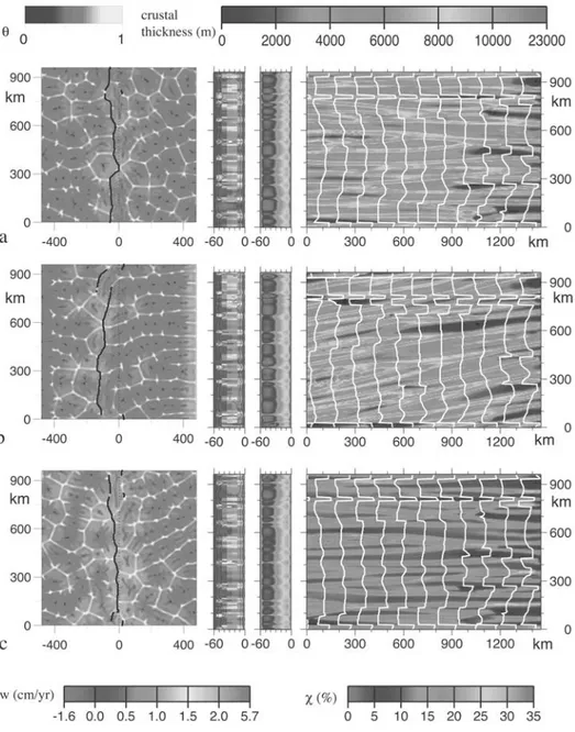
toroidal scalar fields. Then the equation of motion leads to a biharmonic equation and a harmonic equation for the poloidal and toroidal parts, respectively. These equations are solved using a Fourier horizontal decomposition and a vertical finite difference one. This method is detailed by Rabinowicz et al. [1993]. The temperature equation is solved using a finite difference method known to give good results in 3-D modeling of mantle convection [Douglas and Rachford, 1956; Blankenbach et al., 1989]. Convection Figure 2. Comparison of three distinct, 90-Myr-long experiments with a Ra = 30,000, a half-spreading
velocity Vaccr = 17 mm yr"1 and a bottom shear Vbot = 0. In the first two experiments the ridge axis
position is fixed (Figures 2a and 2b), while in the last one it migrates as explained in the text and Appendix A (Figure 2c). In the first model the upwelling driven by plate accretion is not added to the flow field (Figure 2a). The maps at the left represent the final snapshot of the middepth horizontal nondimensional thermal field, bright colors designate hot fluids with close to 1, and dark ones designate cold fluids with close to 0. The initial position of the axis is marked by a north-south dotted line and the final position by solid lines. (right) Isochron and crustal thickness on the eastern flank of the oceanic plate. The isochrons at 8 Myr-interval are drawn in plain white lines, and the crustal thickness is in color. Scales of color for the crustal maps are drawn at the top. The middle left box shows vertical velocity w in the ridge plane and temperature at the end of each experiment. Isotherms are drawn in plain black lines. The middle right box displays melt fraction by weigh along the ridge plane. Color scales for w and for are shown at the bottom. See color version of this figure at back of this issue.
with motionless boundaries and a Rayleigh number ranging between 24,000 and 100,000 has a bimodal flow structure: that is, it consists of the superposition of two sets of orthogonal rolls. However, when we initiate our experi-ments with a random thermal field, we never obtain a perfect set of orthogonal rolls in a reasonable period of time. The time needed to reach the 3-D, asymptotic, steady state regime is proportional to several times the
conductive time D2/k, i.e., several times 160 Myr
[White-head and Parsons, 1978]. Hence we choose to start our numerical experiments with the 16 Ma snapshot of the thermal field of a convective case run with zero top and
bottom shearing velocities (Vaccr = Vbot = 0), and initiated
with the temperature field:
T x; y; zð Þ ¼ Ttopþ Tinf" Ttop
" # z Dþ 0:05sin p z D & ' ranf x; yð Þ h i ; ð15Þ
where ranf (x,y) designates a random function with a unit mean amplitude.
3. Experiment Results
[20] In order to get a progressive insight on the
relation-ships between convection and magmatic or geometric ridge segmentation we present several experiments which differ by the Rayleigh number or by the flow conditions set along the top and bottom interfaces of the computing box. 3.1. Cases With a Small Rayleigh Number and No Bottom Shear
[21] Figure 2a displays a case with a Rayleigh number
Ra = 30,000, a top half-spreading velocity Vaccr= 17 mm yr"1
and a zero horizontal bottom velocity Vbot = 0. In this
experiment the ridge axis is maintained straight and parallel to the y direction and we do not take into account the diffuse flow resulting from plate accretion. At the end of the 90 Ma experiment the convective flow consists in a set of intersect-ing rolls. Over 100 km from the ridge, the rolls whose axes are parallel to the ridge direction are quite damped, and those parallel to the spreading direction concentrate the essential part of the flow and temperature heterogeneity [Richter and Parsons, 1975]. In the following, we designate this last type of rolls as Richter’s rolls. The spacing between the
succes-sive, parallel Richter’s rolls is!110–150 km. Close to the
ridge, there is a continuous set of hot ascending sheets, subparallel to the ridge direction, which zigzag on both sides of the axial plane. In the vicinity of the ridge axis, curving streamlines of the cavity flow induced by the top spreading delineate a roof-shaped domain, where the mantle is fairly still (Figure 1). In fact, this quiescent domain favors the development of these ridge-parallel, hot upwelling sheets. Most of the Richter’s rolls are connected to these sheets. Where they intersect, the flow is strong and hot, producing more crust than elsewhere along the axis (Figure 2a, right). Since the experiment begins with a convective flow which is not symmetrical with respect to the ridge plane, the Richter’s rolls below the eastern and western spreading plates are not necessarily connected to the same ridge-subparallel ascend-ing sheets. The temperature, velocity, and melt fraction along the ridge plane at the end of the experiment reveal that the
flow ascends along most of this plane, except along two narrow zones, above which the crustal production is null (Figure 2a, middle). Note that the mean crustal thickness produced during the 90 Ma experiment is 2 km. Magmatic lineations with a maximal crustal thickness of 9 km are produced above the intersections of Richter’s rolls and ridge-parallel hot sheets.
[22] The introduction of the diffuse flow resulting from
plate accretion drives a uniform, vertical upwelling with a
1.1 mm yr"1 intensity across the bottom boundary of the
computational box. Although this flow does not alter the convective pattern, it does increase the flow intensity in the parallel hot sheets (Figure 2b). Several ridge-parallel upwelling sheets develop even far away from the ridge axis. Because of the strengthening of the spreading orthogonal flow the amplitude of the magmatic lineations increases and the mean crustal production averaged over the 90 Ma experiment reaches 2.3 km.
[23] In the following experiment the ridge axis is
iter-atively adjusted to follow the local maximum of tension generated by the convective circulation (Figure 2c and 3). The experiment is initiated with a straight ridge. The other parameters are those of the last experiment (Figure 2b). The convective circulation evolves slowly: The flow and ther-mal state after 8 Ma consist of a set of intersecting rolls remaining very close to the one used to initiate the experi-ment (Figure 3a). The ascending sheets form a zigzagging
network of planes with a horizontal length of !70 km.
Stronger upwellings at the intersection of ascending sheets form hot plumes. Many of these plumes result from the intersection of two rolls only. However, plumes in which three distinct rolls originate are common. This last feature also occurs during the initiation of analogue laboratory experiments with similar Rayleigh numbers as a result of the ‘‘pinching’’ of two parallel rolls into a single one [Busse and Whitehead, 1974]. As time goes on, top shearing movement progressively reorganizes the flow, decreasing the number of convective rolls. After 90 Ma (Figure 3f ) the spacing between successive parallel Richter’s rolls is 110 – 150 km. It exceeds the initial spacing of the bimodal set of rolls by a factor up to 2 (Figure 3a). We observe that the ridge segments migrate either eastward or westward to sit above the closest ridge-parallel ascending sheet. When the ridge axis meets the ascending flow of a ridge-parallel roll, large continuous ridge segments develop (Figure 3a). The same snapshot shows that ridge segments initially located above Richter’s rolls tend to migrate far from their first position (Figures 3a and 3f ). This leads to the initiation of
U-shaped transform-ridge-transform systems !100 km in
offset. The progressive reorganization of the convective flow leads to the progressive collapse of some transform offsets. Nevertheless, we note that U-shaped systems located above Richter’s rolls are particularly stable (Figure 3). Also, in this experiment, two long ridge seg-ments having captured two different, ridge-parallel rolls remain separated by a 100-km offset transform fault during the whole experiment. At the end of the 90 Ma experiment the ridge line tends to become more continuous and the convective flow structure remains strikingly similar to that obtained when the position of the ridge axis is held fixed (compare Figures 2a, 2b, and 2c,). This similarity suggests that the local adjustment of the ridge position only weakly
modifies the evolution of the convective flow. Figure 2c shows that the ridge segments coincide with the axis of the hot ascending sheets except at the vicinity of a transform offset where the local maximum of tension does not coincide with the roll axis. The convective snapshots show that the different ridge segments remain <100 km from the initial ridge line (Figure 3). The isochron and crustal map associated with this model (Figure 2c) show that the mean crustal production during the 90 Myr duration of the
experi-ment is 3.5 km,!50% thicker than in the experiments with
a fixed ridge axis (Figures 2a and 2b). The increase in crustal thickness results from the fact that most of the ridge axial segments are now positioned above ridge-parallel hot sheets where melt production reaches its maximum. Figure 3 shows that only transient ridge discontinuities migrate along the ridge. Also, magmatic lineations tend to migrate along
axis. Their drift results from the along-strike migration of the subridge hot plumes. They drift very slowly in
compar-ison with the convective velocity: 200 km during!50 Ma
or 0.4 mm yr"1.
[24] Strikingly, we observe several cases where two
magmatic lineations merge (Figure 2c). It occurs when a pinching plume meets the ridge axis, for example, in the northern part of the plate boundary between 24 and 40 Ma (Figures 3b and 3c). The merging occurs when two ridge segments drifting above two distinct rolls ride over a point where the two rolls pinch into one. Conversely, the splitting of a magmatic lineation occurs where the ridge drifts above a spreading-parallel upwelling which then divides into two distinct sheets. The rate of melting, the temperature, and the velocity field on the ridge plane at the end of the experiment show that the mantle flow is ascending below the whole
Figure 3. Evolution of the thermal field when Ra = 30,000, Vaccr= 17 mm yr"1, and Vbot= 0 (model
also shown in Figure 2c), shown as snapshots of the middepth temperature in a window restricted to the central part of the computing box. Plotting conventions are as in Figure 2. See color version of this figure at back of this issue.
ridge axis, except near a small domain in the central part of the plate boundary where the ridge axis sits above a dipping current (Figure 2c). In fact, Figure 3f shows that this ridge segment lies near a transient ridge discontinuity overriding an entire convective cell. As a result, the ridge crustal production is null at the intersection of the ridge axis and the dipping part of this convective cell.
[25] Figure 4a displays the situation when we double the
half-spreading velocity Vaccr to 34 mm yr"1. Other
param-eter values are the same as those of the last experiment. The evolution of the convective circulation and the ridge adjustment observed at 45 Ma (Figure 4a) resembles the one recorded at 90 Ma when the spreading velocity is
17 mm yr"1(Figure 2c). Since most of the flow along the
ridge plane is advected upward by the free convection, the volume of melt produced along the ridge axis remains quite constant (Figure 4a), implying that the mean crustal thick-ness is now 1.8 km, i.e., just over half the mean crustal
production recorded when Vaccr = 17 mm yr"1.
3.2. Experiments With a Small Rayleigh Number and a Bottom Shear
[26] In Figures 4b and 4c we display the evolution of the
flow, the ridge position, and the crustal production when the bottom of the mush layer is sheared to the east with
Vbot= (8 mm yr"1, 0 mm yr"1) and to the southeast with
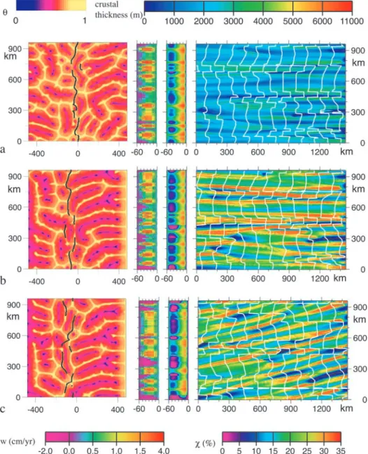
Figure 4. Three distinct experiments with Ra = 30,000. Plotting conventions as in Figure 2. The first
experiment (Figure 4a) shows the effect of doubling the spreading velocity: Vaccr= 34 mm yr"1instead of
17 mm yr"1. In the last two experiments (Figures 4b and 4c) we test the effect of a shear velocity at the
bottom of the layer: Vbot= (8 mm yr"1, 0 cm yr"1) and Vbot= (8 mm yr"1, 8 mm yr"1), respectively. The
experiments in Figures 4b and 4c last 90 Myr, while the one in Figure 4a lasts 45 Myr. Other parameter values are those of the model drawn in Figures 2c and 3. See color version of this figure at back of this issue.
Vbot= (8 mm yr"1, 8 mm yr"1), respectively. The Rayleigh
number and the half-spreading velocity Vaccrare still 30,000
and 17 mm yr"1, respectively. The eastward or the
south-eastward drift of the lower interface leads to a slow, westward migration of the ridge segments. After 90 Ma the ridge segments have been displaced by <100 km, i.e., with a velocity an order of magnitude lower than the eastward drift applied on the lower interface. The south-eastward drift of the lower interface leads to a small asymmetrical rotation of the Richter’s roll on both sides of the ridge axis: anticlockwise along the eastern flank of the ridge and clockwise on its western flank. The magmatic lineations on the eastern flank of the plate now point to the
south (Figure 4c). The obliquity of the lineations with respect to the spreading direction is consistent with the fact that the ridge-parallel bottom shearing moves the Richter’s rolls in the flow direction. The westward drift of the ridge results from westward orientation, beneath the lithosphere, of the cavity flow driven by the eastward shear imposed at the bottom of the computing box (Figure 1). 3.3. Experiments With a Large Rayleigh Number
[27] In Figure 5 we present two models, with a Rayleigh
number Ra of 90,000 and a top half-spreading velocity
Vaccr= 17 mm yr"1. The bottom horizontal flow velocity is
Vbot= 0 in the model of Figure 5a but Vbot= (17 mm yr"1,
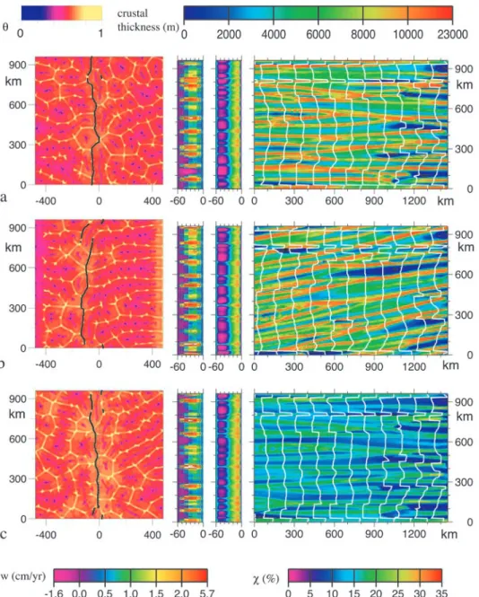
Figure 5. Three distinct experiments with a Ra = 90,000. Plotting conventions are as in Figure 2. The
two first experiments (Figures 5a and 5b) are run with a half-spreading velocity Vaccr= 17 mm yr"1. They
differ by the bottom shear velocity which is equal to Vbot= 0 and to Vbot= (8 mm yr"1, 17 mm yr"1) in
Figures 5a and 5b, respectively. The experiment in Figure 5c shows the effect of doubling the spreading
velocity: Vaccr= 34 mm yr"1instead of 17 mm yr"1(here also Vbot= 0). The experiments in Figures 5a and
8 mm yr"1) in Figure 5b. In the former case, the convective cells form a polyhedral set of ascending hot sheets centered around an area of downwelling flow (Figure 5a). The number of hot sheets forming these polyhedrons varies and reaches a maximum of 8. Each individual hot sheet
keeps a length of !50–90 km and some polyhedrons
exceed 150 km in diameter. Even after 90 Ma, the orienta-tion of the various hot sheets remains independent of the spreading direction (Figure 5a). This is consistent with the fact that the convective velocity, which reaches a maximum
of 60 mm yr– 1, is strong in comparison with the forced
flow velocity, which reaches a maximum speed of only
Vaccr = 17 mm yr"1. This convective structure is striking.
For the same Rayleigh number range, standard Rayleigh-Benard convection displays two intersecting sets of rolls !0.5D–0.7D in width and !1D in length [Frick et al., 1983]. Experiments run with exactly the same parameter values, but in which the diffuse flow resulting from plate accretion is omitted, also develop Richter’s rolls 0.5D – 0.7D in width (models not shown here, and Rabinowicz et al. [1993]). This suggests that it is the diffuse vertical bottom flow induced by the plate thickening which favors the development of the polyhedral flow structure. The ridge axis at the end of the experiment is almost
contin-uous. The crustal lineations are separated by !60 km
(Figure 5b). The splitting or merging of magmatic line-ations is common because of the numerous ‘‘pinched rolls’’ needed to give a polyhedral structure to the convective flow. The crustal production averaged over the whole experiment is 5.9 km. Initially, a large number of dipping currents develop beneath the ridge axis, explaining a relatively weak crustal production. After 40 Ma the crustal production is strong along the entire length of the ridge axis because the whole ridge is then located above ascend-ing hot sheets of the polyhedral convective structure. The crustal production averaged along axis at the end of the experiment is 6.7 km. When the lower interface is sheared to the southeast, the flow still tends to display a polyhedral structure (Figure 5b). Strikingly, we see that along the eastern flank of the ridge, the spreading movement tends to destroy the polyhedrons and drives 100 – 140 km distant Richter’s rolls, while over the western flank, the polyhe-drons are clearly drawn (Figure 5b). This asymmetry results from the fact that when the lower interface is sheared in the direction of spreading, the cavity flow tends to increase the intensity of the shear stress due to spreading along the top boundary, while the opposite effect occurs when the shear acts in the opposite direction (see Figure 1). We also observe that the eastward shear of the lower interface leads to a slow westward drift of the ridge axis and that the southward bottom shear leads to a southward migration of the crustal production centers (Figure 5b). Otherwise, the mean crustal production remains the same as in the case with no bottom shearing (Figure 5a).
[28] In Figure 5c we display the results of an experiment
similar to the one shown in Figure 5a (Ra = 90,000; no
bottom shear, Vbot = 0) but with a faster half-spreading
velocity, Vaccr= 34 mm yr"1. After 44 Myr of shearing at a
spreading rate of 34 mm yr"1 the convective flow is very
similar to the one after a shearing at a 17 mm yr"1velocity
during 90 Ma (Figures 5a and 5c). However, the mean
crustal production is divided by!2 when the plate
spread-ing velocity doubles: 3.6 km at 34 mm yr"1 instead of the
5.9 km of mean crustal production at 17 mm yr"1.
4. Discussion
4.1. Modeling Framework
[29] Although it is now commonly admitted that
small-scale convection occurs in the partially molten mantle beneath the ridge, modeling this process is incredibly diffi-cult. The reason is simple. The small-scale convection interacts strongly with the whole mantle flow and with the generation, percolation, and crystallization of the melt in the upper mantle. In fact, the problem becomes more tractable if we take into account the large amount of evidence showing that the partially molten domain has a viscosity drastically lower than that of the underlying mantle [Rabinowicz et al., 1984; Buck and Su, 1989; Sparks et al., 1993]. This implies that the small-scale mantle convection is ‘‘partially’’ con-fined within the mantle mush. Yet this confinement clearly cannot be complete. First, because of the oceanic plate accretion, material is sucked into the mantle mush. This process is extremely important because it provides the undepleted mantle from which the oceanic crust is extracted [Scott, 1992; Turcotte and Phipps Morgan, 1992; Braun et al., 2000]. Also, part of the large-scale mantle flow driven by hot or cold spots circulates inside the mantle mush [Schilling et al., 1995]. Here we consider that at some distance from hot and cold spots this flow corresponds to a horizontal and regionally constant temperature flow. As shown by Vogt [1976], this flow moves preferentially along the roof-shaped ‘‘valley’’ formed by the accreting oceanic plates. However, when the hot spot is located away from the ridge axis, the flow necessarily moves in a direction transverse to the valley. The mantle melting or crystallization being generated by heating/cooling or by compression/decompression, a large-scale horizontal flow with a locally constant temper-ature does not modify the melting rate. Consequently, the melting process occurs by decompression in the upwelling limbs of the small-scale cells. Meanwhile, the crystallization process occurs by cooling in the top boundary layer and by compression inside the downwelling limbs of the same convective cells. As shown above, these drastic approxima-tions allow us to model the mantle dynamics with a tractable set of equations and boundary conditions.
4.2. Summary of the Main Results of the Modeling
[30] Although the cavity flow induced by the plate
spreading tends to generate Richter’s rolls!200 km from
the ridge plane, the convective circulation is clearly three-dimensional closer to the ridge axis. In fact, the 3-D nature of the flow results from the combined effects of the forced flows driven by plate spreading and plate accretion. Plate spreading generates a roof-shaped domain of quiescent flow around the ridge plane favoring the development of upwell-ing sheets there. The flow driven by plate accretion induces a slow and diffuse vertical flow at the bottom of the mantle mush which strongly enhances the buoyancy of the bottom convective boundary layer. The resulting dissymmetry between the bottom and top convective boundary layers leads to the development of cells with a polyhedral ascend-ing flow structure [White, 1988]. The convective pattern below the ridge is a compromise between (1) Richter’s rolls favored by plate spreading at some distance from the ridge,
(2) upwelling sheets along the ridge plane which develop because of the quiescence of the subridge flow at the bottom of the mush, and (3) polyhedrons favored by the diffuse upwelling flow driven by plate accretion.
[31] Clearly, the observed structures depend on (1) the
Rayleigh number, (2) the spreading velocity, and (3) time. The time required to reach a quasi-steady state structure is almost independent of the Rayleigh number but decreases linearly with the half-spreading velocity. It is roughly equal to
90 and 45 Ma when Vaccr= 17 and 34 mm yr"1, respectively.
Near the ridge axis, however, the convective pattern is governed by the Rayleigh number. A Rayleigh number of !30,000 drives two orthogonal sets of rolls, parallel to the ridge axis and to the spreading direction, respectively. The characteristic width of the rolls increases with time. The
length of the cells is!70 km at the beginning of the
experi-ment and reaches 110 – 150 km at the end. When the Rayleigh number reaches 90,000, the upwellings form polyhedrons with sides 50 – 90 km in length. In our formulation the ridge axis is free to move along the spreading direction and to adjust itself to the shear stresses generated along the litho-sphere-mush interface by the convective circulation [Rouzo et al., 1995]. During the transient period the ridge presents a discontinuous geometry with many U-shaped transform-ridge-transform systems. However, the ridge segments gen-erally tend to realign to form a continuous line located above upwelling sheets of the convective circulation. Below the continuous portions of the ridge axis, the flow forms a set of connected sheets parallel to the ridge. Crustal production is twice as large at the intersection of these sheets as elsewhere along the ridge. Sometimes near a transient discontinuity, a ridge segment can sit temporally above a downwelling current. During this time the crustal production drops to zero along this ridge segment. In the synthetic maps of crustal thickness and isochrons the excess crustal production occur-ring above the intersection of two convective hot sheets produces magmatic lineations subparallel to the spreading direction (Figures 2 – 5). Yet two magmatic lineations often merge into one, or one lineation splits in two. These situations occur when the ridge axis lies over the intersection of three distinct hot ascending sheets. The component of large-scale mantle flow moving in a direction parallel to the ridge axis induces a southward migration of the hot upwelling sheets responsable for the crustal thickness variations. The resulting magmatic lineations form V shapes pointing in the direction of the large-scale flow. Yet a large-scale flow moving in a direction parallel to the spreading direction does not modify the convective structure. In fact, it only reinforces the shear-ing of the convective circulation by the oceanic plate which moves in the same direction. However, this flow component drives the ridge axis in the upstream direction. Note that both the segmentation and drift of the ridge axis induced by the convection in the mush and the shear of the large-scale mantle flow depend on the subridge local structure of convection and recirculation flow. This indicates that our results should remain invariant in a model taking into account the thinning of the mushy layer in the spreading direction.
[32] We have estimated the melting rates in the mantle
and the crustal production at the ridge axis using the formalism of McKenzie and Bickle [1988]. The temper-atures at the top and bottom of the models are adjusted to
reach reasonable melting rates. At a depth of!10 km inside
the mantle mush, the melting fraction reaches a local maximum of 32%. Since we assume that the melt in excess
of mc = 6% is transported by porosity waves to the ridge
axis, the resulting crust is a continuous mixture of melts derived from a parent rock whose melting rates range from 6 to 32% and melting depths range between 10 and 60 km below the bottom of the lithosphere. We have computed the mean melting rate and the averaged depth of melting along the whole ridge plane of model of Figure 5a (i.e., with a Rayleigh number Ra = 90,000, a top half-spreading velocity
Vaccr= 17 mm yr"1, and a bottom velocity Vbot= 0). This
computation yields a mean melt rate of 16% and an averaged melting depth of 31.8 km. Since the top of the mush layer is assumed to be at 15 km below sea level, the average melting depth is at 46.8 km below sea level. These numbers agree with those estimated by Langmuir et al. [1992] and Shen and Forsyth [1995].
4.3. Evaluation of the Mean Crustal Thickness, the Rayleigh Number, and the Rate of Depletion of the Mantle Mush
[33] When the Rayleigh number rises from 30,000 to
90,000, with a half-spreading velocity Vaccr= 17 mm yr"1,
the along-axis mean crustal thickness increases from 3.4 to 6.7 km. These numbers are upper bounds because they have been computed assuming that the mantle advected by the convective circulation is 100% fertile. This is the case when the bottom convective boundary layer is composed entirely
of fertile mantle. Since this layer has a thickness of!8 km
and is fed with fertile mantle by the 1.1 mm yr"1 upward
flow due to the plate accretion, it is completely filled with
fertile mantle in !7 Myr. To transport 100% of fertile
mantle, the ascending flow along the ridge axis would have to be in contact during 7 Myr with the mush-dry mantle interface before moving upward. Because of the large viscosity contrast along the mush-mantle interface, the horizontal mean convective velocity close to this interface
is slow. It is <10 mm yr"1 in the model with a Rayleigh
number of 30,000 and twice as large in the model with a Rayleigh number of 90,000. Because of the 100 – 200 km extension of the convective cells it is likely that the convective current flowing along the 100-km-wide bottom interface of the convective cell remains in contact with this lower interface during the 7-Myr period required to fill it
with fertile mantle. With a Rayleigh number of !90,000,
the convective upwelling provides 75% of fertile material below the ridge, enough to produce a crust 5 km thick on average. When the spreading rate doubles, the velocity of the upward flow due to the plate accretion also doubles. However, the melt flow rate reaching the lithosphere increases slowly because it mainly depends on the fertility rate and on the convective velocity. Thus the mean crustal
production decreases by a factor of !2. A factor of 3
increase of the Rayleigh number is required to double the convective velocity and to match the average 5 km mean crustal production.
[34] To produce a fixed crustal production, we therefore
have two alternatives. Either we assume that the Rayleigh number of the mush layer is much greater than 90,000 and thus that most of the upwelling mantle flow below the ridge axis is composed of depleted material mixed with a constant flow of undepleted material, or we can assume that the
Rayleigh number varies around a value of 90,000 and that it is generally positively correlated with the spreading rate. We have shown above that the Rayleigh number depends mainly on the viscosity of the mush. Thus a variation by a factor of up to 10 in the Rayleigh number could be attributed to variations of a few tens of degrees of the bulk temperature of the mush layer. This estimate of the large-scale temperature variations below the ridge axis is reason-able if we consider that the mush is fed by large-scale convective flows. In the warmest domains the increase of the Rayleigh number increases the production of crust which consequently balances the crustal thinning expected at a faster spreading ridge. Therefore the invariant 5-km crustal thickness observed along most of the Earth’s ridge system could result from the fact that the plate boundaries with the fastest spreading rates are those located above a mantle which is a few tens of degrees hotter. This con-clusion agrees with global studies of the Earth’s ridge system [Lecroart et al., 1997]. Alternatively, if the second interpretation is correct, we can assume that the Rayeigh number of the mush is high in anomalously hot regions like the Icelandic hot spot and low at the Australia-Antarctic Discordance. Then our model can explain why the crustal production is clearly high while the spreading velocity is low at the Icelandic hot spot and why the crustal production is low above the cold though relatively fast spreading center of the Australia-Antarctic Discordance [Forsyth et al., 1987; Sempe´re´ et al., 1991].
4.4. Stability of the Mantle Mush
[35] If we look at the partially molten mantle layer from
below, we see a severe stability problem. In our models the mean temperature of the mush is 150!C lower than in the mantle below it. It is clear that the resulting negative buoy-ancy can be compensated by the positive buoybuoy-ancy of the interstitial melt trapped in the upwelling flow. However, such an effect is not strong enough to ensure the overall stability or even the neutral stability of the whole layer. In other words, the 90 Myr stability of the mantle mush as a whole assumed in our modeling requires some justifications.
[36] The shear flow imposed at the bottom of the partially
molten layer to simulate the coupling with the large-scale flow driven by whole mantle convection is consistent with a layering of the circulation on both sides of the bottom interface of the mush. If the hot spot plume penetrates inside the roof-shaped-mush layer, the resulting cavity flow will turn in a direction opposite to the one driven by mantle flow shearing the bottom interface of the mush. Accordingly, the sense of the ridge axis migration generated by the large-scale mantle flow depends dramatically on the stability of the mush layer. To achieve such stability requires a significant density contrast between the return flow and the overlying depleted mantle, which can only be due to compositional differences. Density contrasts attributable to chemical com-position are essentially related to the Fe/Mg ratio of olivine and pyroxenes in the residual mantle depending themselves on the degree and pressure of melting. The higher the degree of melting, the lower the Fe/Mg ratio, and thus the density, of the residual mantle. For equal melting degrees the Fe/Mg ratio of the residue increases slightly as the pressure of melting increases [e.g., Kinzler, 1997]. The contrast in melting degree between hot spots and ridges is poorly
constrained. Some authors have argued that higher crustal thicknesses at hot spots imply much more partial melting in mantle plumes than beneath mid-ocean ridges [McKenzie and Bickle, 1988; White et al., 1992; Langmuir et al., 1992]. This should be reflected in lava composition. Although slight differences in composition between hot spot lavas and mid-ocean ridge basalts (MORBs) exist, they can be attributed to pressure effects and to the dynamics of melt migration [Liu and Chase, 1991; Ceuleneer et al., 1993; Putirka, 1999]. High crustal thicknesses at hot spots can also result from 3-D focusing of mantle flow [Ribe and Chris-tensen, 1994]. The best guess is that the average melting degree is somewhat similar in both environments, particu-larly when the hot spot is located below a relatively thick lithosphere. There is no doubt, however, that the pressure of melting contrasts strongly. Accordingly, we can expect a residue richer in Fe, and hence denser material, in hot spots. Variations in the pressure of melting can also induce density contrasts in the residue related to mineralogy. The contribu-tion of olivine and pyroxenes to the melt varies with pressure: the higher the pressure of melting, the higher the proportion of olivine entering in the melt phase, the lower the olivine/pyroxene ratio, and thus the density, of the residue [Herzberg and Zhang, 1996]. This effect will lower the density of the residual mantle in hot spots relative to ridges, an effect that will counteract and perhaps even balance the one related to the Fe/Mg ratio. In both ridge and hot spot settings, but particularly where a hot spot is overlain by a thick lithosphere, the melt extraction is not complete. Thus part of the melt will remain trapped in layers and eventually crystallize in layers as the temperature drops away from the upwelling currents. In the shallow environ-ments (ridges) these layers will crystallize as pyroxenites and gabbroic cumulates with lower densities than the surround-ing mantle [Ceuleneer et al., 1996]. Below 50 km depth, they will crystallize as garnet pyroxenites and eclogites which are possibly 30% denser than the surrounding mantle [Gregoire et al., 1994; Kinzler, 1997]. Near the bottom interface of the mush beneath a ridge axis, the flow advected by the hot spot should be rich in garnet pyroxenite and eclogite layers. We expect that these layers generate 1% of density contrast between the mush and underlying mantle. Such contrast in density is large enough to ensure the layering of the large-scale and small-scale convection on both sides of the bottom interface.
4.5. Modeling Perspectives
[37] Although we have tried to retain the essential
physics known to act in the dynamics of the mantle mush, our modeling draws a partial picture of the geological situation because of the drastic simplifications needed to obtain a tractable set of equations. However, future work should be done to evaluate the effects of realistic rheological laws for the mantle mush, of melt percolation, and of crystallization. Also, future work should be concerned with the precise modeling of the interaction between small-scale convection in the mush and whole mantle convection.
5. Comparison Between Models and Data
[38] In this section we compare our numerical
experi-ments to observations on the flanks of mid-ocean ridges presented by Briais and Rabinowicz [2002].
5.1. Along-Axis Variations of the Crustal Production and Segment Length
[39] Our model successfully predicts along-axis
varia-tions of the crustal production of the order of several
kilometers. These variations define magmatic segments which are not always bounded by ridge offsets. The devel-opment of a ridge magmatic segmentation in the absence of an offset is an intrinsic characteristic of the model. Ridge segment centers are located above maxima of crustal thick-ness production because of favorable temperature and vertical velocity conditions (see along-axis sections in Figures 2 – 6). Crustal thickness average obtained for
sim-ulations with a half-spreading rate of 17 mm yr"1, the
average value for the southern Mid-Atlantic Ridge (MAR),
and Ra of 30,000 or 90,000 are !3.5 and !6.7 km,
respectively. The higher value is close to the 6-km average crustal thickness estimated for mid-ocean ridges [Mutter and Mutter, 1993]. The crustal thicknesses estimated in our model show variations in the range 0 – 20 km, larger than those estimated at mid-ocean ridges, which barely reach 5 km. One explanation for that discrepancy is that our model does not include any along-axis melt redistribution or crustal flow. These effects are suspected to occur at ridges, although their mechanism is not well documented [e.g., Bell and Buck, 1992; Lawson et al., 1996].
[40] The resulting wavelength of the segmentation is
!110–150 km for Ra of 30,000 and 50–90 km for Ra of 90,000. For low Rayleigh numbers the upwellings corre-spond to intersections of convective rolls parallel to the ridge with the Richter rolls parallel to spreading. For higher Ra values the upwellings are located at the junctions of three to four polyhedral convective cells and are thus more closely spaced. The data analysis presented by Briais and Rabinowicz [2002] reveals that the ridge axis segment length is 50 km on average. Such a wavelength for the axial segmentation is closer to that obtained in our experi-ments with Ra of 90,000 than for the lower Ra. Segexperi-ments of the northern Central Indian Ridge (CIR) are slightly shorter, but they are separated by large-offset transform faults, so that the distance between spreading cells is closer to 100 km. Our current model does not address the effect of transform faults on segment length or that of a strong obliquity between the ridge and the spreading direction. The eastern-most section of the ultraslow spreading Southwest Indian Ridge has longer segments than average, reaching 130 – 200 km as estimated from mantle Bouguer gravity analysis [Rommevaux-Jestin et al., 1997]. This region appears to be one of the coldest parts of that ridge and should be compared to our low-Ra experiments.
5.2. Evolution of the Segmentation Geometry
[41] In our model, series of segments develop above the
upwelling sheets that are subparallel to the spreading ridge. Distinct series of segments located above two different upwelling sheets are usually separated by a large-offset discontinuity. Such discontinuities tend to be very stable in space, although the offset across them varies, whereas small offsets tend to migrate along axis. This contrast between two types of geometrical discontinuities is observed along the mid-ocean ridges, where transform faults tend to be stable enough to record the plate motion vector, whereas nontransform discontinuity traces are obli-que to plate flow lines.
[42] The offsets between segments above the same
upwelling sheet tend to decrease with time, so that at the Figure 6. Mantle flow, isochrones, and magmatic
linea-tions when a hot spot located beneath the ridge crest drives a very strong north-south mantle flow. Parameter values are those of the North Atlantic plates next to the Icelandic hot
spot. The half-spreading velocity is 8.5 mm yr"1. The
Rayleigh number of the experiment Ra = 90,000. The
bottom shear velocity Vbot = (0 mm yr"1, 70 mm yr"1).
The experiment is initiated with the 90 Ma snapshot of the temperature field of Figure 5a experiment. (bottom left) The ridge plane isolines at the end of the experiment for vertical velocity w, temperature, and the melt fraction by weigh. (bottom right) The 90 Ma maps of the crustal lineations and isochrons. The crustal thickness is 13 km on average. (top) Several snapshots of the middepth temperature in a window restricted to the central part of the computing box. Note the development of major transform faults. Plotting conven-tions are as in Figure 2. See color version of this figure at back of this issue.