CSI based indoor localization using Ensemble Neural Networks

HAL Id: hal-02334588

https://hal.archives-ouvertes.fr/hal-02334588

Submitted on 4 Nov 2019

HAL is a multi-disciplinary open access

archive for the deposit and dissemination of

sci-entific research documents, whether they are

pub-lished or not. The documents may come from

teaching and research institutions in France or

abroad, or from public or private research centers.

L’archive ouverte pluridisciplinaire HAL, est

destinée au dépôt et à la diffusion de documents

scientifiques de niveau recherche, publiés ou non,

émanant des établissements d’enseignement et de

recherche français ou étrangers, des laboratoires

publics ou privés.

CSI based indoor localization using Ensemble Neural

Networks

Abdallah Sobehy, Eric Renault, Paul Muhlethaler

To cite this version:

Abdallah Sobehy, Eric Renault, Paul Muhlethaler. CSI based indoor localization using Ensemble

Neu-ral Networks. MLN 2019 : 2nd IFIP International Conference on Machine Learning for Networking,

Dec 2019, Paris, France. pp.367-378, �10.1007/978-3-030-45778-5_25�. �hal-02334588�

Neural Networks

Abdallah Sobehy1_{, Éric Renault}1_{, and Paul Mühlethaler}2

1

Samovar, CNRS, Télécom SudParis, University Paris-Saclay, 9 Rue Charles Fourier, 91000 Évry, France.

sobehy@telecom-sudparis.eu, eric.renault@telecom-sudparis.eu

2

INRIA Roquenourt, BP 105, 78153 Le Chesnay Cedex, France Paul.Muhlethaler@inria.fr

Abstract. Indoor localization has attracted much attention due to its indispensable applications e.g. autonomous driving, Internet-Of-Things (IOT), and routing, etc. Received Signal Strength Indicator (RSSI) was used intensively to achieve localization. However, due to its temporal instability, the focus has shifted towards the use of Channel State In-formation (CSI) aka channel response. In this paper, we propose a deep learning solution for the indoor localization problem using the CSI of a 2 × 8 Multiple Input Multiple Output (MIMO) antenna. The variation of the magnitude component of the CSI is chosen as the input for a multi-layer Perceptron (MLP) neural network. Data augmentation is used to improve the learning process. Finally, various MLP neural networks are constructed using different portions of the training set and different hy-perparameters. An ensemble neural network technique is then used to process the predictions of the MLPs in order to enhance the position estimation. Our method is compared with two other deep learning so-lutions; one that uses Convolutional Neural Network (CNN), and the other uses MLP. The proposed method yields higher accuracy than its counterparts.

Key words: Indoor Localization, Channel State Information, MIMO, Deep Learning, Neural Networks

1 Introduction

Localization is the process of determining the position of an entity in a given coordinate system. Knowing the position of devices is essential for many appli-cations; autonomous driving, routing, environmental surveillance etc. The local-ization system depends on multiple factors. The environment, whether indoors or outdoors, is one of the most dominant factors. In outdoors environment, Global Positioning System (GPS) is widely used to localize nodes. In [1], the authors present a location service which targets nodes in a Mobile Ad-hoc Net-work (MANET). The aim is to use the GPS position information obtained at each device and disseminate this information to other nodes in the network while

avoiding network congestion. Each node broadcasts its position with higher fre-quency to nearby nodes and lower frefre-quency to further nodes. The notion of closeness is determined by the number of hops. This way, nodes have more up-dated position information of nearby nodes which is sufficient for routing appli-cations, for instance. While the GPS satisfies the requirements for many outdoor applications, it is not functional in indoors environment. Consequently, in such scenarios, other measurements have to be exploited to overcome the absence of GPS.

A family of localization methods is known as range-based localization. In this method, a physical phenomenon is used to estimate the distance between nodes. Then, geometrically the relative positions of nodes within a network can be computed [2]. One of the most used phenomenons is the Received Signal Strength Indicator (RSSI). RSSI is an indication of the received signal power. It is mainly used to compute the distance between a transmitter and a receiver since the signal strength decreases as the distances increases. In [3], the distances between nodes along with the position information of a subset of nodes, known as the anchor nodes, are used to locate other nodes in a MANET. This is achieved using a variant of the geometric triangulation method. The upside of RSSI is that it does not need extra hardware to be computed and is readily available. Another physical measure to compute distance between devices is the Time-Of-Arrival (TOA) or Time-Difference-Time-Of-Arrival (TDOA). Here, the time taken by the signal to reach the receiver is used to estimate the distance between devices. Using TOA in localization proves to be more accurate, but requires external hardware to synchronize nodes [4]. In the case where only the distance information is available, a minimum of three anchor nodes with prioirly known positions are needed to localize other nodes with unknown positions. In order to relax this constraint, the Angle-Of-Arrival (AOA) information can be used in addition with distance. Knowing the angle allows to localize nodes with only one anchor node [5]. However, the infrastructure needed to compute AOA is more expensive than TOA both in terms of energy and cost.

Even though RSSI has been extensively used in indoor localization [6], it exhibits weak temporal stability due to its sensitivity to multi-path fading and environmental changes [6]. This leads to a relatively high error in distance es-timation which, in turn, deteriorates the position eses-timation accuracy. With the data rate requirements of the 5g reaching up to 10 Gbps, the communica-tion trend is switching to the use of MIMO antennas where signals are sent on multiple antennas simultaneously [7]. Furthermore, with orthogonal frequency-division multiplexing (OFDM), each antenna receives multiple signals on ad-jacent subcarriers. This introduces the possibility of computing a finer-grained physical phenomenon at the receiver which is known as Channel State Infor-mation (CSI). In other words, as opposed to getting one value per transmission with RSSI, with CSI, it is possible to estimate CSI values which are equal to the number of antenna × the number of subcarriers. CSI represents the change that occurs to the signal as it passes through the channel between the transmitter and the receiver e.g. fading, scattering and powerloss [8]. Equation (1) elaborates the

relation between the transmitted signal Ti,j and the received signal Ri,j at the

ith _{antenna and the j}th _{subcarrier. The transmitted signal is affected by both}

the channel through the CSIi,j, which is a complex number, and the noise N .

Ri,j= Ti,j· CSIi,j+ N (1)

2 Related Work

One of the very first attempts to use CSI for indoor localization is FILA [9]. With 30 subcarriers, the authors compute an effective CSI which represents the 30 CSI values at each of the subcarriers. Then they present a parametric equation that relates the distance to the effective CSI. The parameters of the equation are deduced using supervised learning. Finally, using a simple triangulation tech-nique, the position is estimated. In [10], the authors carry an experiment where a robot carrying a transmitter traverses a 4 × 2 meter table and communicates with an 8 × 2 MIMO antenna. The transmission frequency is 1.25 GHz and the bandwidth is 20 MHz. Signals are received at each of the 16 subantennas over 1024 subcarriers from which 10 % are used as guard bands. Using a convolutional neural network (CNN), the authors use the real and imaginary components of the CSI as an input to the learning model to estimate the position of the robot. The authors publish the CSI and the corresponding positions readings which are used as the test bed for our algorithm. Therefore, the comparison with their results is fair since both algorithms process the same data. Figure 1 shows the experimental setup as well as a sketch of the MIMO antenna and the position of its center.

Another solution that is tested on the same data set is NDR [11] which is based on the magnitude component of the CSI. First, the magnitude values are preprocessed by fitting a line through the points. Then a reduced number of magnitude points are chosen on the fitted line to represent the whole spectrum of CSI. By achieving this, both the dimensionality of the input and the noise are reduced. Since our solution is based on the same basis, we will provide a brief explanation of the preprocessing step.

In Section 3, the building blocks of the proposed solution are introduced. First, the choice of magnitude component and the data preprocessing steps are briefly explained. Second, the data augmentation step is presented followed by the ensemble neural network technique. The localization accuracy of our solu-tions is compared with two state-of-the-art solusolu-tions in section 4. Finally, the conclusion and future work are discussed in Section 5.

3 Methodology

3.1 Learning Model Input

Since the CSI is a complex number, it can be represented in both polar and cartesian forms. Thus, there are a total of four components to represent the

Fig. 1. Experimental setup (bottom) and a sketch of the MIMO antenna (top) [10]

CSI; real, imaginary, magnitude, and phase. Equations (2) and (3) show the conversion from one form to another.

CSIi,j = Re + iIm (2)

M ag =pRe2_{+ Im}2

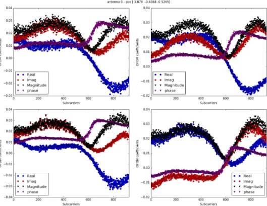
φ = arctan(Re, Im) (3) A good input feature is one that is stable for the same position. In other words, if the transmission occurs multiple times from the same position, the fea-ture values are expected to be similar. In order to examine the behaviour of the components, the four components are plotted for four different transmissions from the same position. Figure 2 shows the CSI components of four different transmissions from the same position. Each sub-figure shows the four CSI com-ponents of one transmission. It is to be noted that the phase values are all scaled to be in the same order as the other components. With a careful inspection, it can be notices that the magnitude component shows the highest stability. This

conclusion is further supported by the analysis performed in [11, 12]. Conse-quently, we chose the magnitude to be the input component to the deep learning model.

Fig. 2. Real, Imaginary, Magnitude and phase components estimated from 4 trans-missions from the same position.

3.2 Data Preprocessing

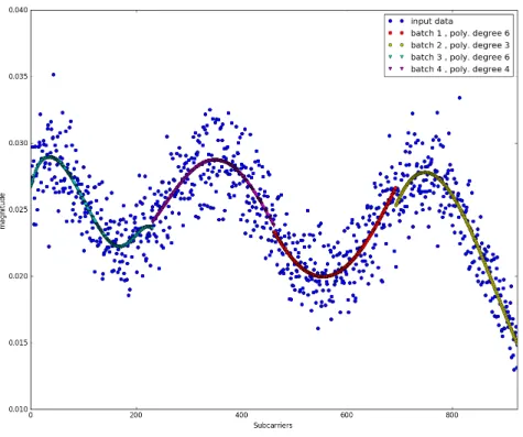
After choosing the magnitude as the input feature, the number of input values to estimate one position is 924 × 16. As seen in figure 2, the magnitude points appears to follow a continuous line with noise scattering points around this line. The first step is to retrieve a line that passes through the magnitude values. Since this process has to be performed for each of the 15k training samples multiplied by the 16 antennas, it has to be relatively fast. This process is achieved by polynomial fitting on four sections over the subcarrier spectrum [11]. Figure 3 shows the four batches, each with a different color, and the degree of the polynomial used to fit the line. The polynomial degree is chosen by attempting several values and choosing the degree that yields the highest accuracy. Dividing

the spectrum into four sections increases the accuracy of the overall fitting. More details of the fitting process can be found in [11].

Fig. 3. Fitting a line through the magnitude values.

The following steps is to use a reduced number of points along the fitted lines instead of the whole set of 924 points. This mitigates the noise that leads to the scattering around the line. In addition, the reduction allows to build a more complex MLP that trains in less time. In [11], 66 points are used to represent the whole spectrum. We chose the input feature to be the difference (slope) between two consecutive points. For the 66 points, there are 65 slope values. Using the same MLP structure in [11], the mean square error is reduced from 4.5 cm to 4.2 cm over a 10-fold cross validation experiment. Even though this is a slight improvement of around 7%, it shows that the absolute value of the magnitude is not the decisive factor to determine the position, but rather the variation of the magnitude along the spectrum.

3.3 Data Augmentation

Data augmentation is a method to increase the training set which is the main driver for the learning process. The artificially created training samples are con-structed from the available samples with some mutation. In image recognition context; blurring, rotating, zooming in or out are all ways to generate a new training sample from an existing one.

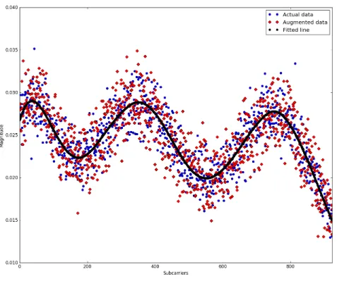
In our case, a training sample is composed of a set of 924 × 16 magnitude points and the corresponding position. In our solution we propose the mutation to the input and the output sides of the training sample. As for the output posi-tion, we know the measuring error of the tachymeter used to calculate the given position which is around 1 cm [10]. We model this error by a Gaussian distri-bution with zero mean, which is the given position, and a standard deviation which is 1/3 cm. Thus, the position of the augmented sample is computed using this distribution. As for the magnitude points, first, a line is fitted through the points with the previously mentioned method. Next, the standard deviation of the absolute error between the line and the values is computed. The augmented sample is then calculated by scattering the points around the fitted line with a Gaussian distribution with zero mean and two times the computed standard deviation. This can be seen as an equivalent to the blurring in the image recog-nition context. Figure 4 shows an example of an augmented magnitude sample in red from an original training sample in blue using a fitted line in black.

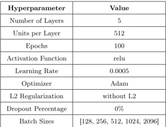
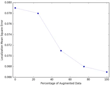
In order to test the effect of data augmentation on localization accuracy, an MLP neural network is constructed with the hyperparameters listed in Table 1. Training the MLP is then executed with different percentages of augmented data. Figure 5 shows the effect of the number of augmented data samples on the mean square error of the position estimation.

Table 1. Hyperparameters selection.

Hyperparameter Value

Number of Layers 5

Units per Layer 512

Epochs 100

Activation Function relu

Learning Rate 0.0005

Optimizer Adam

L2 Regularization without L2

Dropout Percentage 0%

Fig. 4. Data augmentaion sample from an original training sample.

It is worth mentioning that the larger the augmented data set, the better the localization accuracy. The mean square error is reduced from 8 cm to 6.7 cm using an augmented sample from each training sample.

3.4 Ensemble Neural Networks

The last piece of our algorithm is to construct several neural networks with different characteristics. The difference between MLPs can be in the hyperpa-rameters or the training samples used to train the model. For instance, the neural networks used to plot Figure 5 are different since they are trained on different training sample sizes. Also, in k-fold cross validation, neural networks are trained on the same data size but on different samples. Moreover, changing any of the hyperparameters shown in Table 1 leads to different results.

Mixing the prediction of each neural network with different characteristics can lead to a significant increase in accuracy. We examine different ways to mix the prediction results of the MLPs:

Fig. 5. Effect of data augmentation on localization accuracy.

1. Mean: The simplest way to mix the results is to compute the arithmetic mean position of all the predictions.

2. Weighted mean: Each of the MLPs are given a weight that is proportional to its individual localization accuracy. Thus, the higher the accuracy, the higher the weight. Then the final prediction is a weighted average of the individual prediction.

3. Weighted power mean: The effect of weights is further magnified by raising them to a certain power before computing the weighted average.

4. Median: The idea is to pick one of the predictions that is closest to all other predictions. This makes sense when the ensemble has three or more MLPs. This mitigates the effect of the large errors of some predictions.

5. Random: The final prediction is a randomly selected individual prediction. 6. Best pick: This is used as an indication of the best possible result one can

attain with the given ensemble. The final prediction is the closest individual prediction to the actual position. This is not feasible since in normal cases the actual position is not given.

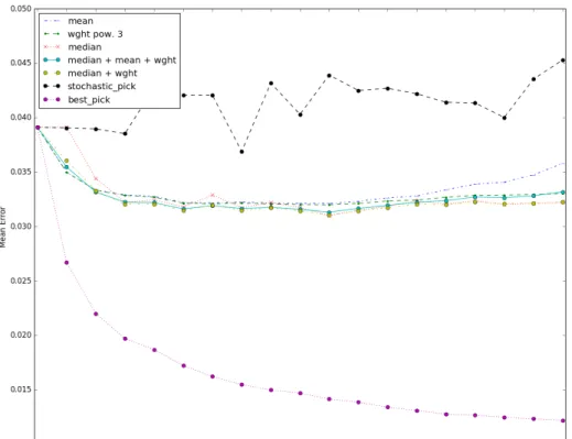
Figure 6 shows the effect of adding a neural network to the ensemble. The x-axis represents the number of the neural networks in the ensemble. Beside the number of the NNs, there is a number between brackets representing the mean square error of the added neural network. This means that the first MLP has a Mean Square Error (MSE) of 3.9 cm. This the best individual MLP which was constructed using the data augmentation technique. The y-axis shows the MSE for each type of predictions mixing. One of the types in Figure 6 is labeled "median + wght" meaning the average prediction of both mixing methods. It can be seen that with different mixing techniques, except for the random pick,

the estimation accuracy can be improved even if the added MLP has a higher individual error. The best achieved accuracy is 3.1 cm MSE using 11 MLPs. This result outperforms [10] that uses a CNN learning from real and imaginary components and achieves an error of 32 cm. It also outperforms [11] which uses an MLP learning from the magnitude values and achieves an error of 4.5 cm. It is to be noted that the accuracy can be still increase if there is a way to select the best individual estimation of the MLPs ensemble.

Fig. 6. Mixing the predictions of a neural network ensemble.

4 Experimental Results

In this section, we compare the localization accuracy of the proposed Ensemble NN method based on the variation of magnitude and data augmentation with

NDR [11] and CNN [10] methods. NDR is an MLP where the input is the magnitude values, and the hyperparameters are chosen emperically to get the lowest mean square error estimation. CNN is a convolutional network where the input is the real and imaginary components of the CSI. The estimation results in NDR and CNN are presented while varying the number of used antennas in estimation.

Fig. 7. Comparing Ensemble NN with NDR [11] and CNN [10]

As expected, when lower number of antennas is used the estimation error is high. In all solutions the estimation improves with more data provided from the added antennas. The proposed Ensemble NN technique outperforms NDR and CNN. The error of CNN is much higher than NDR and Ensemble NN probably due to the high temporal instability of the real and imaginary CSI components. While the error difference between NDR and CNN seem small, the improvement is relatively significant. When using 16 antennas, NDR achieves an MSR of 4.3 cm while the proposed Ensemble technique achieves 3.1 cm which is an improvement of ≈ 30%.

5 Conclusion

In this work, we propose a deep learning solution for the indoor localization problem based on the CSI of a 2 × 8 MIMO antenna. The variation of the mag-nitude component is chosen to be the input feature for the learning model. Using the magnitude variation instead of the absolute values improves the estimation slightly. This shows that the focus should be to better describe the change in magnitude along the subcarrier spectrum rather than the absolute values. Data augmentation is then used to further increase the estimation accuracy. Finally, an ensemble neural network technique is presented to mix results of different MLPs and achieves an accuracy of 3.1 cm outperforming two state-of-the-art solutions [10, 11]. This work can be improved through the detection and correc-tion of outliers as some of the errors are much larger than the mean error. The possibility of using another learning layer to detect outliers or select the best individual MLP estimation from the ensemble might enhance the estimation accuracy.

References

1. Renault, Eric, Ebtisam Amar, Hervé Costantini, and Selma Boumerdassi. "Semi-flooding location service." In Vehicular Technology Conference Fall (VTC 2010-Fall), 2010 IEEE 72nd, pp. 1-5. IEEE, 2010.

2. Čapkun, Srdjan, Maher Hamdi, and Jean-Pierre Hubaux. "GPS-free positioning in mobile ad hoc networks." Cluster Computing 5, no. 2 (2002): 157-167.

3. A. Sobehy, E. Renault, and P. Muhlethaler, "Position Certainty Propagation: A Localization Service for Ad-Hoc Networks." Computers 8, no. 1, 2019. 6.

4. Nandakumar, Rajalakshmi, Krishna Kant Chintalapudi, and Venkata N. Padman-abhan. "Centaur: locating devices in an office environment." In Proceedings of the 18th annual international conference on Mobile computing and networking, pp. 281-292. ACM, 2012.

5. Cidronali, Alessandro, Stefano Maddio, Gianni Giorgetti, and Gianfranco Manes. "Analysis and performance of a smart antenna for 2.45-GHz single-anchor indoor positioning." IEEE Transactions on Microwave Theory and Techniques 58, no. 1 (2009): 21-31.

6. Yang, Zheng, Zimu Zhou, and Yunhao Liu. "From RSSI to CSI: Indoor localization via channel response." ACM Computing Surveys (CSUR) 46, no. 2 (2013): 25. 7. Jungnickel, Volker, Konstantinos Manolakis, Wolfgang Zirwas, Berthold Panzner,

Volker Braun, Moritz Lossow, Mikael Sternad, Rikke Apelfrojd, and Tommy Svens-son. "The role of small cells, coordinated multipoint, and massive MIMO in 5G." IEEE communications magazine 52, no. 5 (2014): 44-51.

8. He, Suining, and S-H. Gary Chan. "Wi-Fi fingerprint-based indoor positioning: Re-cent advances and comparisons." IEEE Communications Surveys & Tutorials 18, no. 1 (2015): 466-490.

9. K. Wu, J. Xiao, Y. Yi, M. Gao and L. M. Ni, "Fila: Fine-grained indoor localization." In 2012 Proceedings IEEE INFOCOM, pp. 2210-2218. IEEE, 2012.

10. M. Arnold, J. Hoydis and S. T. Brink, "Novel Massive MIMO Channel Sounding Data applied to Deep Learning-based Indoor Positioning." In SCC 2019; 12th Inter-national ITG Conference on Systems, Communications and Coding, pp. 1-6. VDE, 2019.

11. Abdallah Sobehy, Eric Renault, Paul Muhlethaler. NDR: Noise and Dimensionality Reduction of CSI for Indoor Positioning using Deep Learning. GlobeCom, Dec 2019, Hawaii, United States. (hal-023149)

12. X. Wang, L. Gao, S. Mao and S Pandey, "DeepFi: Deep learning for indoor finger-printing using channel state information." 2015 IEEE wireless communications and networking conference (WCNC), pp. 1666-1671. IEEE, 2015.