HAL Id: tel-02869772
https://tel.archives-ouvertes.fr/tel-02869772
Submitted on 16 Jun 2020HAL is a multi-disciplinary open access archive for the deposit and dissemination of sci-entific research documents, whether they are pub-lished or not. The documents may come from teaching and research institutions in France or abroad, or from public or private research centers.
L’archive ouverte pluridisciplinaire HAL, est destinée au dépôt et à la diffusion de documents scientifiques de niveau recherche, publiés ou non, émanant des établissements d’enseignement et de recherche français ou étrangers, des laboratoires publics ou privés.
Analyse probabiliste des règles de vote : méthodes et
résultats
Abdelhalim El Ouafdi
To cite this version:
Abdelhalim El Ouafdi. Analyse probabiliste des règles de vote : méthodes et résultats. Economies et finances. Université de la Réunion, 2019. Français. �NNT : 2019LARE0037�. �tel-02869772�
1
UNIVERSITÉ DE LA RÉUNION
Faculté de Droit et d'Économie
Centre d’Economie et de Management de l’Océan Indien
Thèse de sciences économiques Présentée par : Abdelhalim El Ouafdi
Analyse probabiliste des règles de vote :
méthodes et résultats.
Date : 09/12/2019
Composition du Jury
M. Christophe Depoortère Professeur à l’université de La Réunion Examinateur M. Mostapha Diss Professeur à l’université de Franche-Comté Rapporteur M. Michel Le Breton Professeur à l’université Toulouse 1 Capitole Examinateur M. Dominique Lepelley Professeur à l’université de La Réunion Directeur de
thèse M. Hatem Smaoui Maître de conférences HDR, à l’université de La
Réunion
Directeur de thèse
2 L’université n’entend donner aucune approbation ni improbation aux opinions émises dans les thèses : ces opinions doivent être considérées comme propres à leurs auteurs.
3 À la mémoire de mon père et de mon grand-père
4
Remerciements
Au terme de ce travail doctoral je tiens à exprimer ma reconnaissance et mes chaleureux remerciements envers l’ensemble des personnes qui, à un moment ou à un autre, d’une manière ou d’une autre, ont contribué à l’aboutissement de ce travail doctoral grâce à leur soutien et leur aide.
Mes remerciements et ma reconnaissance s’adressent tout d’abord à mes directeurs de thèse Monsieur Dominique Lepelley et Monsieur Hatem Smaoui sans qui ce travail n’aurait pu voir le jour.
Mon parcours n’aurait sûrement pas été le même sans leur patience, bienveillance, confiance et encouragement. Ils ont toujours étaient disponible, à l’écoute de mes nombreuses questions et se sont toujours intéressé à l’avancée de mes travaux. Les nombreuses discussions et échange que nous avons eues, ainsi que leurs explications sont pour beaucoup dans le résultat final de ce travail. Cette thèse leur doit beaucoup.
Mes remerciement les plus chaleureux vont également au professeur Nicolas Gabriel Andjiga et au professeur Issofa Moyouwou, de m'avoir accueilli à L'ENS Yaoundé pour un séjour de recherche. J'en garde des moments très agréable.
Mes remerciements vont également aux différents membres du jury : les Professeurs Mostapha Diss et Fabrice Valognes qui ont accepté la tâche d’évaluer ce travail doctoral, les professeurs Christophe Depoortère et Michel Le Breton pour avoir accepté de prendre part au jury de soutenance. Leurs commentaires seront sources d’enrichissement pour mes travaux futurs. Qu’ils trouvent ici l’expression de ma respectueuse reconnaissance.
Je remercie chaleureusement la faculté de sciences économiques et à travers elle la structure de recherche CEMOI, de m’avoir accueilli en son sein et de m'avoir permis de réaliser cette thèse. Je remercie également les personnes qui m'ont aidé à se loger et à bien s'installer au début de mes études universitaires. Je leur suis reconnaissant.
Je remercie également tous les doctorants et tous les autres membres du laboratoire CEMOI, ainsi que les membres de l'ENS Yaoundé et tous ceux que j'ai pu côtoyé et avec qui j'ai pu partager de bons moments.
5 Je remercie affectueusement ma famille pour son attention, soutien et encouragement, tout au long de ce travail de recherche.
La recherche est une passion. J'ai eu la chance durant mes études d'avoir eu de merveilleux professeurs qui, par leur cours, disponibilité, et échange, ont nourris en nous étudiants l'esprit de curiosité et d’ouverture sur ce monde passionnant qu'est la science. Je leur témoigne ma plus grande gratitude et ma reconnaissance.
6
Table des matières
Introduction ... 9
1. Vote et paradoxes ... 9
2. La probabilité des paradoxes ... 15
3. Objet et plan de la thèse ... 18
4. Références ... 20
Chapitre 1 - IAC-Probability Calculations in Voting Theory: Progress Report ... 23
1. Introduction... 23
2. Probabilities calculations under the IAC condition ... 26
3. The algebraic Approach ... 28
4. The geometric approach for limiting probabilities ... 31
5. Huang-Chua method and EUPIA procedure ... 33
6. Ehrhart theory based methods ... 35
7. Concluding remarks ... 39
8. References ... 40
Chapitre 2 - Probabilities of electoral outcomes : From three candidate to four candidate elections ... 45
1. Introduction... 45
2. Voting rules and electoral outcomes ... 46
3. Methodology ... 49
4. Results on Condorcet conditions ... 52
5. Results on coalitional manipulability ... 58
6. Concordance of all scoring rules ... 61
7. Conclusion ... 63
8. Appendix: Computation of Pr(𝐸3, ∞) ... 64
7 Chapitre 3 - On the Condorcet Efficiency of Evaluative Voting (and other Voting Rules) with
Trichotomous Preferences ... 71
1. Introduction and motivation ... 71
2. Extending Scoring Rules and Approval Voting to the trichotomous framework... 74
3. Results on the Condorcet winner efficiency with trichotomous preferences ... 76
4. Condorcet Loser Election and other results with trichotomous preferences ... 82
5. Conclusions and final remark ... 85
6. References ... 88
Chapitre 4 - Manipulabilité coalitionnelle du vote par note à trois niveaux ... 91
1. Introduction... 91
2. Préférences trichotomiques et manipulation stratégique ... 92
3. Vulnérabilité de EV, PR, NPR et BR à la manipulation coalitionnelle... 98
4. Considérations méthodologiques ... 110
5. Conclusion ... 113
6. Bibliographie ... 114
7. Annexe ... 115
Conclusion générale ... 118
Annexe A : Code - Trichotomous preferences ... 121
Annexe B : Code - Probabilities of electoral outcomes : From three candidate to four candidate elections ... 128
8 S’il est une question centrale qui peut être envisagée comme la problématique principale motivant la théorie du choix social, c’est la suivante : comment est-il possible de parvenir à des jugements agrégés et incontestables au niveau de la société... – Amartya Sen [36]
9
Introduction
1. Vote et paradoxes
1.1 Vote majoritaire et paradoxe de Condorcet
L’agrégation des préférences individuelles en une préférence collective est une problématique importante dans la théorie économique moderne. Le choix social en a fait une question centrale. La sélection de la meilleure alternative globale parmi un ensemble d’alternatives a été étudiée depuis longtemps et sous diverses formes.
Dans un processus d’élection avec deux candidats, la majorité est la meilleure règle de vote. Le candidat élu est celui qu’une majorité d’électeurs préfère à l’autre. En 1952, May [28] en donne une caractérisation et une justification théorique : pour lui, dans un choix binaire avec deux options, la règle de la majorité est la seule règle de décision qui est à la fois neutre, anonyme, monotone et non manipulable. En d’autres mots, c’est une règle qui ne favorise ou désavantage aucun des deux candidats, où les électeurs sont égaux et sont incités à exprimer leurs vraies préférences.
Cependant, avec trois candidats ou plus, l’agrégation des préférences en un choix collectif pose quelques problèmes. En 1785, Condorcet1 [9], dans son Essai sur l’application de l’analyse à la probabilité des décisions rendues à la pluralité des voix, souligne les difficultés de l’agrégation de préférences et d’opinions individuelles en un choix collectif. Il a montré que le vote majoritaire peut conduire à une préférence collective non transitive et cyclique : il peut arriver lors d’une élection qu’un candidat A soit préféré à un autre candidat B par une majorité d’individus, qu’une autre majorité de votants préfère B à C, et qu’une autre encore préfère C à A. Donc les décisions prises peuvent ne pas être cohérentes avec celles que prendrait un individu rationnel, car le choix entre A et C ne serait pas le même selon que B est présent ou non. Ceci est historiquement le premier exemple de paradoxe de vote, on parle de paradoxe de Condorcet ou, suivant Guilbaud [19], de l’effet Condorcet. Par paradoxe, on désigne ici un résultat contre-intuitif auquel on peut aboutir à l’issu d’un scrutin, ou un phénomène allant à l’encontre de ce que dicterait la conformité sociale, plutôt qu’une contradiction purement
1 Marie Jean Antoine Nicolas Caritat, marquis de Condorcet, est un mathématicien et homme politique français,
représentant des Lumières, né le 17 septembre 1743 à Ribemont en Picardie et mort le 29 mars 1794 à Bourg-la-Reine
10 logique. L’exemple original présenté par Condorcet d’une situation de vote avec 60 électeurs et trois candidats est le suivant :
23 17 2 10 8
𝐴 𝐵 𝐵 𝐶 𝐶
𝐵 𝐶 𝐴 𝐴 𝐵
𝐶 𝐴 𝐶 𝐵 𝐴
Table 1
Lorsqu’on effectue les comparaisons majoritaires par paires, ce système nous donne que : A est préféré à B (33–27),
B est préféré à C (42–18), C est préféré à A (35–25).
Ainsi, A ≻ B ≻ C ≻ A (le symbole ≻ désignant la préférence collective). On appelle cette situation un cycle de Condorcet. Chaque candidat est battu par au moins un autre ; il n’existe donc pas de vainqueur de Condorcet, c’est- à-dire de candidat capable de l’emporter à la majorité sur chacun de ses concurrents.
Le vainqueur de Condorcet peut donc ne pas exister. Notons cependant que, sous certaines conditions, on peut outrepasser ce paradoxe de Condor- cet. Par exemple lorsque les préférences sont unimodales2, l’existence d’un vainqueur de Condorcet est garantie.
1.2 Borda et les règles positionnelles
Borda3, qui était le contemporain de Condorcet, propose une approche alternative dite de classement par points. Dans la méthode qu’il propose, les électeurs construisent chacun une liste de n candidats par ordre de préférence. Le premier de la liste, reçoit n points, le second n-1 points, et ainsi de suite, le nième de la liste se voyant attribuer n-1 point. Le score d’un candidat est alors la somme de tous les points qui lui ont été attribués. Le (ou les) candidat(s) dont le score est le plus élevé remporte(nt) l’élection. La règle de la pluralité (ou de la majorité simple),
2 La condition d’unimodalité a été introduite par Black [5]. Elle revient à exclure certains ordres de préférences. 3 Jean-Charles, chevalier de Borda, né le 4 mai 1733 à Dax et mort le 19 février 1799 à Paris, est un
11 qui consiste à donner 1 point pour une première place et 0 point pour toute autre position, constitue comme la règle de Borda une méthode de classement par points ; ces méthodes sont aussi appelées règles positionnelles simples. Cette famille de règles a la particularité de garantir la condition de consistance. C’est-à-dire que si un électorat est partagé en deux groupes, et si un candidat est le vainqueur dans chaque groupe, alors ce dernier va rester le vainqueur si les deux groupes sont réunis. Cette propriété de consistance constitue un argument fort en faveur de l’utilisation des règles de classement par points. Cependant, ces règles ne respectent pas toujours le critère dit de Condorcet (ou critère majoritaire) : le vainqueur peut ne pas être le vainqueur de Condorcet (lorsque celui-ci existe).
Ce qu’on appelle le paradoxe de Borda résulte d’une observation très intéressante concernant les conflits possibles entre le principe majoritaire et la règle de la pluralité pour déterminer le vainqueur d’une élection. L’exemple original de Borda [6] en ce qui concerne ce phénomène utilise la situation de vote de la table 2 pour 21 électeurs avec des préférences strictes et transitives lors d’une élection à trois candidats.
1 7 7 6
𝐴 𝐴 𝐵 𝐶
𝐵 𝐶 𝐶 𝐵
𝐶 𝐵 𝐴 𝐴
Table 2
Si on utilise la règle de la pluralité, on aura A ≻ B (8–7), A ≻ C (8–6) et B ≻ C (7–6), soit le classement A ≻ B ≻ C. Un résultat très différent est observé en utilisant la règle de la majorité. On a B ≻ A (13–8), C ≻ A (13–8) et C ≻ B (13–8), donc C ≻ B ≻ A (notons que le candidat A constitue ici ce qu’on appelle un perdant de Condorcet). Selon qu’on utilise la règle de la pluralité ou le principe majoritaire, le classement final sera inversé.
1.3 Le cas du vote majoritaire à deux tours
Parmi les méthodes de choix collectif, le vote majoritaire à deux tours est une règle très intéressante. Elle est utilisée dans de nombreux pays, et particulièrement en France pour l’élection présidentielle. Avec cette règle, on a un bulletin uninominal. Au premier tour, le candidat qui obtient plus de la moitié des voix est déclaré vainqueur, sinon les deux candidats
12 ayant reçu le plus de voix vont au second tour. Au second tour, le candidat avec le plus de voix est élu. Un exemple pour illustrer cette méthode est présenté dans la table 3.
10 6 5
𝐴 𝐵 𝐶
𝐵 𝐶 𝐵
𝐶 𝐵 𝐴
Table 3
Au premier tour, A et B obtiennent un score de 10 et 6 (respectivement), et C n’obtient qu’un score de 5. Comme A n’a pas la majorité absolue, A et B vont au second tour. Au second tour, B est élu avec un score de 11 contre 10 pour A.
Un des avantages du vote majoritaire à deux tours est qu’il n’élit jamais le perdant de Condorcet. Cependant, comme toute autre règle de vote, il présente un certain nombre d’inconvénients. Par exemple il ne respecte pas le critère de Condorcet : il arrive dans certaines élections que le vainqueur ne soit pas celui qui est préféré par la majorité. Au-delà du viol du critère de Condorcet, le vote majoritaire à deux tours présente l’inconvénient de ne pas être « monotone » [24], c’est-à-dire que ce système de vote peut réagir de manière contre-intuitive face à de légères modifications des préférences des votants.
6 5 4 2
𝐴 𝐶 𝐵 𝐵
𝐵 𝐴 𝐶 𝐴
𝐶 𝐵 𝐴 𝐶
Table 4
Dans la table 4, A et B vont au second tour et A est élu avec un score de 11 contre 6 pour B. Supposant maintenant que 2 électeurs changent leurs préférences au profit du candidat A et que l’on obtienne les préférences montrées dans la table 5 :
13 8 5 4 𝐴 𝐶 𝐵 𝐵 𝐴 𝐶 𝐶 𝐵 𝐴 Table 5
Au premier tour, les scores de A, B et C sont respectivement 8, 4 et 5. Donc A et C vont au second tour et C est vainqueur avec un score de 9 contre 8 pour A. Par conséquent, ce n’est plus A mais C qui l’emporte : dans un vote majoritaire à deux tours, gagner des suffrages peut ainsi faire perdre l’élection. Ce qui est contraire au bon sens.
Un autre défaut du scrutin majoritaire à deux tours est qu’il est manipulable : certains électeurs sont incités à exprimer une préférence non sincère.
Exemple : 10 6 5 𝐵 𝐶 𝐴 𝐴 𝐴 𝐷 𝐶 𝐵 𝐵 𝐷 𝐷 𝐶 Table 6
Au premier tour, A est éliminé. B et C vont au second tour et B est vainqueur avec 15 voix contre 6 pour C.
Dans la table 6, 6 votants peuvent être incités à changer leur préférence, passant de (C préféré à A préféré à D préféré à B) à (A préféré à C préféré à D préféré à B). On obtient la table 7 : 10 6 5 𝐵 𝐴 𝐴 𝐴 𝐶 𝐷 𝐶 𝐷 𝐵 𝐷 𝐵 𝐶 Table 7
14 Au premier tour, c’est maintenant C qui est éliminé et au second tour, c’est A qui est élu. Donc certains votants, qui préfèrent A à B, sont gagnants en mentant sur leur préférence.
Au-delà de ces inconvénients, le vote majoritaire à deux tours peut présenter aussi d’autres problèmes (absence d’incitation à la participation, non consistance ou encore dictature de la majorité) ; nous renvoyons sur ce point à S. Konieczny [26].
Il existe bien sûr d’autres règles que le vote majoritaire à deux tours, comme le vote par approbation, la règle de Weber, le jugement majoritaire [3] ou encore le scrutin de Condorcet randomisé [22]... Toutes ces règles de vote comportent des avantages et des inconvénients et sont susceptibles d’exhiber des paradoxes. La littérature du choix social les a largement étudiés. Le lecteur pourra consulter par exemple Felsenthal [13], Nurmi [31] [30], Saari [33], Gehrlein et Lepelley [16] [17] pour une revue exhaustive de ces paradoxes.
On peut bien sûr se demander si ces paradoxes sont propres à certaines règles de vote, ou s’il existe une règle qui en serait dépourvue. La réponse à cette question est hélas négative : Arrow [1] en 1951, par son célèbre théorème d’impossibilité, affirme qu’il n’existe pas de processus de choix social indiscutable, qui permette d’exprimer, à partir de l’agrégation des préférences individuelles, une hiérarchie des préférences qui soit cohérente. De manière plus précise, dès que le nombre de choix possibles est supérieur ou égal à 3, il n’existe pas de fonction de choix social qui, simultanément, satisfait aux conditions d’universalité, de transitivité, d’unanimité, d’indépendance et de non dictature. Le théorème d’Arrow a engendré une très vaste littérature, dont on peut trouver un aperçu dans Kelly [25], Sen [37], Fishburn [14].
Il existe par ailleurs dans la littérature d’autre théorèmes d’impossibilités, tel que le théorème de Gibbard-Satterthwaite (Gibbard [18] , Satterthwaite [34]), qui établit que toutes les fonctions de choix social sont manipulables,ou encore le théorème de Sen [35] qui montre qu’on ne peut concilier le principe de Pareto et un libéralisme minimal. Tous ces théorème généralisent en quelque sorte la découverte de Condorcet en montrant qu’il n’y a pas de règles d’agrégation qui peuvent satisfaire un certain ensemble de propriétés ou de principes (Niemi et Riker [29] ) qu’il paraît raisonnable de respecter (comme on l’a vu, avec le paradoxe de Condorcet, c’est la transitivité qui n’est pas respectée quand on applique le vote majoritaire).
15
2. La probabilité des paradoxes
Face à ces théorèmes d’impossibilité, il est naturel de se demander si les fréquences d’occurrences des différents paradoxes qu’ils décrivent sont réellement significatives, ou s’ils sont seulement une sorte de curiosité ma- thématique. Par fréquence d’occurrence, on fait référence au nombre total de situations de vote où l’événement est susceptible de se produire, divisé par le nombre total de situations de vote possibles. La littérature dans ce domaine est très riche ; Gehrlein et Lepelley [16] [17] en présentent un panorama complet.
Les travaux de calcul de probabilités en théorie du vote considèrent deux types d’événements élémentaires : d’abord les profils, qui sont des listes ordonnées de préférences individuelles, puis les situations de vote, qui sont des profils anonymes (seuls comptent les nombres d’électeurs ayant telle ou telle préférence ; l’identité de ces électeurs n’intervient pas, comme dans les exemples donnés ci-dessus). Deux modèles principaux sont alors utilisés :
• Le modèle de culture neutre (IC) (Impartial Culture) :
Guilbaud [19] l’utilise le premier. Sous l’hypothèse (IC), tous les profils sont supposés avoir la même probabilité d’apparition. Cette probabilité est donc de (1
𝑚!)
𝑛où m est le nombre d’options et n le nombre de votants.
• Le modèle de culture neutre et anonyme IAC (Impartial Anonymous culture) :
Introduit par Gehrlein et Fishburn [15] en 1976, il suppose que chaque situation de vote a la même probabilité de se produire, une situation de vote étant définie comme une distribution des électeurs sur les préférences possibles.
D’autres modèles existent : culture duale (DC), culture maximale (MC),... (Voir Gehrlein Lepelley [16]). Notre travail se situe explicitement dans le cadre du modèle IAC. Pour calculer la probabilité d’un événement (de vote) sous l’hypothèse IAC, on considère le cadre formel suivant :
- Un ensemble de n votants : 1, 2, ..., n - Un ensemble de m candidats : A, B, C, ...
- La préférence d’un votant est décrite par un ordre linéaire sur l’ensemble des candidats (classement complet, anti symétrique et transitif)
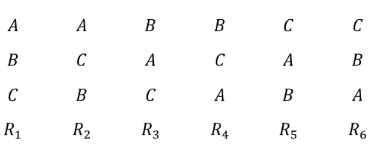
- Pour m = 3, il y a 6 ordres de préférence possibles comme dans la figure 1. Les six ordres sont numéroté de 𝑅1 à 𝑅6. On désigne aussi par 𝑛𝑖 le nombre d’électeurs ayant l’ordre préférence 𝑅𝑖.
16
𝐴 𝐴 𝐵 𝐵 𝐶 𝐶
𝐵 𝐶 𝐴 𝐶 𝐴 𝐵
𝐶 𝐵 𝐶 𝐴 𝐵 𝐴
𝑅1 𝑅2 𝑅3 𝑅4 𝑅5 𝑅6
Figure 1 – ordres de préférence
- Pour m = 4 on a 24 ordres, et 120 pour 𝑚 = 5 ; plus généralement, pour m candidats on a 𝑚! ordres ou préférences individuelles possibles.
- Un profil de préférences individuelles est une liste (ordonnée) de n ordres linéaires.
Dans ce cadre, si on considère un ensemble de m candidats et un nombre n de votants, on peut déduire que le nombre de situations de vote est donné par :
|𝑉(𝑛, 𝑚)| = (𝑛 + 𝑚! − 1 𝑚! − 1 )
En conséquence, pour calculer la probabilité d’un événement (de vote) sous l’hypothèse IAC, il suffit de calculer le nombre de situations correspondantes et de le diviser par le nombre total de situations|𝑉(𝑛, 𝑚)|. Formellement, pour m candidats et pour un événement de vote 𝐸, et (𝐸, 𝑛, 𝑚) l’ensemble des éléments de 𝑉(𝑛, 𝑚) où 𝐸 se réalise, la probabilité d’occurrence de 𝐸, en présence de n votants, est donnée par :
Pr(𝐸, 𝑛, 𝑚) =|(𝐸, 𝑛, 𝑚)| |𝑉(𝑛, 𝑚)|
Souvent le nombre de votant est grand, donc on s’intéresse aussi à la probabilité limite :
Pr(𝐸, ∞, 𝑚) = lim
𝑛→∞Pr(𝐸, 𝑛, 𝑚)
Un événement de vote 𝐸 se présente généralement sous la forme d’un système de contraintes linéaires à coefficients rationnels sur les variables 𝑛𝑖 et dépendant du paramètre n.
Ainsi, l’événement E : « A est le vainqueur de Condorcet » est décrit par le système suivant :
{ 𝑛1+ ⋯ + 𝑛6= 𝑛 𝑛𝑖 ≥ 0,𝑖 = 1, … , 6 𝑛1+ 𝑛2+ 𝑛5 > 𝑛3+ 𝑛4+ 𝑛6 𝑛1+ 𝑛2+ 𝑛3 > 𝑛4+ 𝑛5+ 𝑛6
17 Pr(𝐸, 3, 𝑚) =|(𝐸, 3, 𝑚)|
|𝑉(3, 𝑚)|
Les techniques pour calculer la probabilité Pr(𝐸, 3, 𝑚) sont diverses ; elles se ramènent au dénombrement des solutions entières du système décrivant 𝐸.
La première méthode employée pour effectuer ce calcul est une méthode algébrique qui a été proposée par Gehrlein et Fishburn [1976]. Elle est basée sur l’utilisation des multi-sommes. Ils obtiennent :
Pr(𝐸, ∞, 𝑚) =15 16
Généralement, cette méthode de multi-somme est basée sur des calculs algébriques qui peuvent devenir fastidieux avec l’augmentation du nombre de candidats. Cependant, elle peut se révéler très judicieuses dans certaines situations : sa structure algébrique peut permettre des simplifications intéressantes dans le cas de généralisation à m candidats.
D’autres techniques ont été développées. Ainsi, Huang et Chua [23] (2000) ont montré que les solutions d’un système de contraintes linéaires à coefficients rationnels et dépendant d’un paramètre n se présentent sous forme d’un polynôme en n et à coefficients périodiques. Wilson et Pritchard [32] (2007) et Lepelley, Louichi et Smaoui [27] (2008) introduisent la théorie d’Ehrhart [11] (1967) et montrent que ce polynôme est associé à des polynômes d’Ehrhart, c’est-à-dire qu’un système linéaire à coefficients rationnels décrit un polytope, et que le paramètre n n’est que le coefficient de dilatation de ce dernier. Ainsi le résultat proposé par Huang et Chua n’est qu’un cas particulier d’une théorie plus vaste introduite il y a plus de 40 ans par le mathématicien français Eugène Ehrhart.
La connexion avec la théorie d’Ehrhart a ramené les calculs probabilistes sous IAC à un cadre mathématique bien connu : les polytopes (rationnels) et les quasi-polynômes. Ceci a permis l’introduction d’algorithmes et de techniques de calculs associés à la théorie et d’Ehrhart et aux polytopes dans la théorie du vote, tels que Clauss [8], Barvinok [38], LattE [10] (2004), ou encore Normaliz [7] (2012). L’algorithme le plus utilisé dans la littérature du choix social est celui qui est fondé sur la théorie de Barvinok [4] (1994).
18
3. Objet et plan de la thèse
L’objectif principal de cette thèse est d’optimiser les techniques de calcul des probabilités des paradoxes et de les appliquer à des questions non encore élucidées.
Au cours de ce travail, on a pu calculer un certain nombre de fréquences d’occurrence jusqu’ici inconnues. Pour y parvenir, nous proposons de nouvelles approches de calcul, qui ont pu bénéficier à la fois d’un progrès technique concernant les algorithmes de calcul et aussi du progrès des machines de calcul elles-mêmes, qui sont devenues plus puissantes qu’auparavant.
Notre thèse s’articule en quatre chapitres, de la manière suivante.
Dans le premier chapitre, nous présentons une description de l’évolution des différentes méthodes de calcul utilisées pour obtenir, sous l’hypothèse IAC, les probabilités d’occurrence des paradoxes du vote. Ce survol de la littérature récente a été écrit en collaboration avec Issofa Moyouwou et Hatem Smaoui. Le document associé est soumis pour publication en tant que chapitre d’ouvrage dans un livre à paraître chez Springer. On peut noter que cette contribution a été rédigée après les autres, mais il nous a semblé cohérent de la présenter avant les autres.
Le deuxième chapitre s’intéresse aux paradoxes du vote qui peuvent survenir dans des élections à quatre candidats. La probabilité d’occurrence de ces paradoxes (sous l’hypothèse IAC) a été obtenue par les travaux antérieurs en considérant, le plus souvent, le cadre d’élections à trois candidats. On va dans ce chapitre tenter d’étendre ces calculs au cadre d’élections à quatre candidats, avec par conséquent 24 ordres (linéaires) de préférence possibles. On retrouvera quelques résultats obtenus très récemment par d’autres chercheurs et on proposera de nombreux résultats nouveaux, concernant diverses règles de vote (incluant la règle de Borda et le vote majoritaire à deux tours) et divers paradoxes. Ce chapitre a été écrit en collaboration avec Dominique Lepelley et Hatem Smaoui. Il a été accepté pour publication dans Theory and Decision.
Le troisième chapitre est, techniquement, dans la continuité du deuxième. On s’y s’intéresse au vote par évaluation à trois valeurs (ou vote par note à trois niveaux). Cette méthode de vote a été introduite par Felsenthal (1989) [12] et Hillinger (2004, 2005) [20][21]. Elle fait partie de
19 la large famille des méthodes de vote par évaluation. Selon Balinski et Laraki (2007) [2], et Hillinger (2004), ce genre de méthode cardinale d’agrégation, basée sur le principe d’évaluation, est préférable à l’approche ordinale des préférences individuelles, dans le sens où cette dernière est source de la plupart des paradoxes en théorie du vote. L’étude des paradoxes relatifs à cette règle présente ainsi un intérêt a la fois théorique et technique. Concrètement, le vote par évaluation à trois valeurs est une règle où chaque électeur évalue chaque candidat et lui attribue une note choisie dans l’ensemble 2,1,0. Le gagnant est le candidat qui obtient le plus grand nombre de points. Cette règle a beaucoup de bonnes propriétés, mais elle ne choisit pas systématiquement le vainqueur de Condorcet, c’est-à-dire le candidat (lorsqu’il existe) qui bat chacun des autres candidats dans des comparaisons majoritaires. En supposant que les préférences des électeurs sont de nature trichotomique, et en supposant qu’il n’y a que trois candidats, on se propose dans le chapitre 3 de mesurer et quantifier l’occurrence d’apparition de ce genre de situations, en considérant diverses conditions majoritaires (de type Condorcet) que ne vérifie pas le vote par évaluation. Ce chapitre a été co-écrit avec Dominique Lepelley et Hatem Smaoui. Il est en révision pour la revue Annals of Operations Research.
On conserve dans le chapitre 4 le cadre des préférences trichotomiques avec trois candidats, mais en considérant que les électeurs peuvent voter de manière stratégique. L’étude de la manipulabilité des règles de vote a fait l’objet d’une abondante littérature en théorie du vote. Cependant, il n’existe à ce jour aucune étude permettant de quantifier la manipulabilité théorique des règles de vote par évaluation. Le chapitre 4 se propose de mesurer la manipulabilité du vote par évaluation à trois niveaux, et de comparer cette manipulabilité à celles d’autres règles usuelles (Pluralité, Borda...) que l’on pourrait utiliser dans un contexte de préférences trichotomiques. On propose aussi une nouvelle technique de calcul, qui permet de simplifier considérablement la détermination des fréquences d’occurrence des événements de vote. La contribution associée à ce chapitre a bénéficié des conseils de Jérôme Serais, de l’université de Caen. Qu’il en soit ici remercié.
Nous concluons la thèse avec un résumé des différents résultats obtenus et en soulignant les limites des méthodes et techniques de calcul actuelles.
20
Références
[1] K. J. Arrow, Social choice and individual values. Wiley & Sons, 1951.
[2] M. Balinski and R. Laraki, “A theory of measuring, electing, and ran- king”, PNAS, vol. 104, no. 21, pp. 8720–8725, 2007.
[3] ——, Majority Judgment : Measuring, Ranking, and Electing. MIT Press, 2011. [4] A. I. Barvinok, “A polynomial time algorithm for counting integral points in polyhedra when the dimension is fixed”, Mathematics of Operations Research, vol. 19, no. 4, pp. 769– 779, 1994.
[5] D. Black, “On the rationale of group decision-making,” Journal of Political Economy, vol. 56, no. 1, pp. 23–34, 1948.
[6] J.-C. Borda, Mémoire sur les Elections au Scrutin. Histoire de l’Académie Royale des Sciences, 1781.
[7] W. Bruns, B. Ichim, T. Romer, R. Sieg, and C. Söger, “Library normaliz.” [Online]. Available : https://github.com/Normaliz
[8] P. Clauss, V. Loechner, and D. Wilde, Deriving Formulae to Count Solutions to Parameterized Linear Systems using Ehrhart Polynomials : Applications to the Analysis of Nested-Loop Programs, 1997.
[9] N. de Condorcet, Essai sur l’application de l’analyse à probabilité des décisions
rendues à la pluralité des voix, 1785.
[10] J. De Loera, M. Köppe, and al, “Library latte, ver. 1.5,” 2011. [Online]. Available : http://www.math.ucdavis.edu/latte/
[11] E. Ehrhart, “Sur un problème de géométrie diophantienne linéaire,” Journal für die reine
und angewandte Mathematik (Crelles Journal), vol. 2, no. 227, pp. 25–49, 1967.
[12] D. S. Felsenthal, “On combining approval with disapproval voting”, BS Behavioral
Science, vol. 34, no. 1, pp. 53–60, 1989.
[13] ——, “Review of paradoxes afflicting procedures for electing a single candiyear”,
Felsenthal D., Machover M. (eds) Electoral Systems. Studies in Choice and Welfare, pp. 19–
91, 2012.
[14] P. C. Fishburn, “Interprofile conditions and impossibility”, Harwood Academic
Publishers, 1987.
[15] W. V. Gehrlein and P. C. Fishburn, “The probability of the paradox of voting : A computable solution”, Journal of Economic Theory, vol. 13, no. 1, pp. 14–25, 1976.
21 [16] W. V. Gehrlein and D. Lepelley, Voting Paradoxes and Group Coherence. Springer, 2011.
[17] ——, Elections, Voting Rules and Paradoxical Outcomes. Springer, 2017.
[18] A. Gibbard, “Manipulation of voting schemes : A general result”, Econometrica, vol. 41, no. 4, pp. 587–601, 1973.
[19] G.-T. Guilbaud, “Les théories de l’intérêt général et le problème logique de l’agrégation”, Revue économique, vol. 63, no. 4, pp. 659–720, 2012.
[20] C. Hillinger, On the possibility of democracy and rational collective choice. Univ., Volkswirtschaftl. Fak., 2004.
[21] ——, “The case for utilitarian voting”, vol. 11, no. 23, pp. 295–321, 2005.
[22] L. N. Hoang, “Strategy-proofness of the randomized Condorcet voting system”, Social
Choice and Welfare, vol. 48, no. 3, pp. 679–701, 2017.
[23] H. C. Huang and V. C. H. Chua, “Analytical representation of probabilities under the IAC condition”, Social Choice and Welfare, vol. 17, no. 1, pp. 143–155, 2000.
[24] O. Hudry, “Votes et paradoxes : les élections ne sont pas monotones !” Mathématiques
et sciences humaines, no. 163, 2003.
[25] J. S. Kelly, Arrow impossibility theorems. Academic Pr., 1978.
[26] S. Konieczny, “Une (courte) introduction à la théorie du choix social”, document en ligne, 2008.
[27] D. Lepelley, A. Louichi, and H. Smaoui, “On Ehrhart polynomials and probability calculations in voting theory”, Social Choice and Welfare, vol. 30, no. 3, pp. 363–383, 2008. [28] K. O. May, “A set of independent necessary and sufficient conditions for simple majority decision”, Econometrica, vol. 20, no. 4, pp. 680–684, 1952.
[29] R. G. Niemi and W. H. Riker, “The choice of voting systems”, Scientific American, vol. 234, no. 6, pp. 21–27, 1976.
[30] H. Nurmi, Comparing Voting Systems. D.Reidel, 1987.
[31] ——, Voting paradoxes and how to deal with them. Springer, 1999.
[32] G. Pritchard and M. C. Wilson, “Exact results on manipulability of positional voting rules”, Social Choice and Welfare, vol. 29, no. 3, pp. 487–513, 2007.
[33] D. Saari, Basic geometry of voting. Springer, 1995.
[34] M. A. Satterthwaite, “Strategy-proofness and arrow’s conditions : Existence and correspondence theorems for voting procedures and social welfare functions”, Journal of
22 [35] A. Sen, “The impossibility of a paretian liberal”, Journal of Political Economy, vol. 78, no. 1, pp. 152–157, 1970.
[36] ——, “La possibilité du choix social [Conférence Nobel]”, Revue de l’OFCE, vol. 70, no. 1, pp. 7–61, 1999.
[37] A. K. Sen, “Social choice theory”, Handbook of mathematical economics, vol. 3, pp. 1073–1181, 1986.
[38] S. Verdoolaege, “Library barvinok, ver. 0.34”, 2011. [Online]. Available : http://barvinok.gforge.inria.fr/
23
Chapter 1 : IAC-Probability Calculations in Voting Theory: Progress
Report
Abstract. Over the past two decades, IAC probability calculations techniques have made
substantial progress, particularly through methodological studies that have linked these calculations to their appropriate mathematical framework. We report on this progress by a brief description of the methods of calculation used in this field, and by reviewing some of the results that the application of these methods made possible to obtain.
1. Introduction
In voting theory, probabilistic analysis aims to assess the frequency with which various electoral outcomes can be observed. The primary motivation is, in one hand, to quantify the potential impact of voting paradoxes on real-word elections, and on the other hand, to compare the alternative voting rules on the basis of their ability to meet certain normative criteria. These quantitative results can of course be obtained, in the form of estimates, by empirical and experimental methods (via actual election data and computer simulations).4 However, the most significant part of the research on this topic makes use of analytical methods in order to obtain exact results describing the theoretical probabilities of the voting events under investigation. The book by Gehrlein (2006), entirely devoted to the famous Condorcet Paradox, and the two books by Gehrlein and Lepelley (2011, 2017), in addition to containing the most complete and essential literature reviews on the subject, constitute an excellent illustration of the richness and dynamism of this line of research. William Gehrlein and Dominique Lepelley are certainly the two most eminent and most prolific authors in this field, and one of the main objectives of this paper is also to pay tribute to their fundamental contribution to the probabilistic analysis of voting paradoxes and voting rules.
4
A good summary of empirical and experimental studies can be found in Gehrlein (2006) and Gehrlein and Lepelley (2011). See also Regenwetter et al. (2006), Tideman and Plassmann ( 2012, 2014), Gehrlein et al. (2016, 2018) and Brandt et al. (2016, 2020).
24 The analytical approach uses theoretical models based on certain assumptions about the voters’ preferences. In the literature, the most often used probabilistic models are the Impartial Culture condition (IC), introduced by Guilbaud (1952), and the Impartial Anonymous Culture condition (IAC), described initially by Kuga and Nagatani (1974) and formalized by Gehrlein and Fishburn (1976).5 Over the past two decades, IAC probability calculation techniques have
made substantial progress, particularly through methodological studies that have linked these calculations to their appropriate mathematical framework (Huang and Chua, 2000 ; Cervone et al., 2005 ; Pritchard and Wilson, 2007 ; Lepelley et al., 2008). In this paper, we wish to report on this progress, by a brief description of the methods of calculation used in this field, and by reviewing some of the results that the application of these methods made possible to obtain. For the sake of simplicity, we have chosen to restrict the themes of these representative results to four issues that are among the most often addressed by the probabilistic analysis of electoral outcomes: the election of the Condorcet winner, the election of the Condorcet loser, the (non)monotonicity of voting rules, and finally their manipulability.
In general, these specific voting events are described and studied in a very simple formal framework where individual preferences are represented by linear orderings on the set of candidates. For example, with three candidates (𝑎, 𝑏, and 𝑐), there are six possible individual preference rankings: 𝑎𝑏𝑐, 𝑎𝑐𝑏, 𝑏𝑎𝑐, 𝑏𝑐𝑎, 𝑐𝑎𝑏, and 𝑐𝑏𝑎 (the notation 𝑎𝑏𝑐 means that 𝑎 is preferred to 𝑏, 𝑏 is preferred to 𝑐 and, by transitivity, 𝑎 is preferred to 𝑐). With 𝑛 voters and 𝑚 candidates, a profile is an ordered list of 𝑛 individual preferences chosen from the 𝑚! possible rankings ; a voting situation is an anonymous profile. IC model assumes that each individual preference ranking (and so each profile) is equally likely to be observed. IAC assumes that each possible voting situation is equally likely to be observed. An (anonymous) voting rule is defined as a function that associates a winning candidate with each voting situation.
Most of the studies that will be presented in this brief report deal with voting rules that belong to the class of weighted scoring rules (𝑊𝑆𝑅s) or to the class of scoring elimination rules (𝑆𝐸𝑅s). With 𝑚 candidates, a 𝑊𝑆𝑅 is defined by a scoring vector (𝜆1, 𝜆2, ⋯ , 𝜆𝑚), 𝜆1 ≥ 𝜆2 ≥ ⋯ ≥ 𝜆𝑚 and 𝜆1 > 𝜆𝑚, such that each candidate receives 𝜆𝑘 points each time he/she is ranked 𝑘𝑡ℎ by a voter. The candidate with the most total points wins. The most common 𝑊𝑆𝑅s are plurality rule, 𝑃𝑅 (𝜆1 = 1 and 𝜆𝑘 = 0 for 𝑘 > 1), negative plurality rule, 𝑁𝑃𝑅 (𝜆𝑚 = 0 and 𝜆𝑘 = 1 for 𝑘 < 𝑚), and Borda rule, 𝐵𝑅 (𝜆𝑘= (𝑚 − 𝑘) (𝑚 − 1)⁄ ). In three-candidate election, the scoring
25 vector is of the form (1, 𝜆, 0), 0 ≤ 𝜆 ≤ 1, and we have 𝜆 = 0 for 𝑃𝑅, 𝜆 = 1 for 𝑁𝑃𝑅, and 𝜆 = 1 2⁄ for 𝐵𝑅. Scoring elimination rules use 𝑊𝑆𝑅s in a multi-stage process of sequential elimination : in each stage, the candidate with the lowest total points is eliminated. With three candidates, a 𝑊𝑆𝑅 is used in a first round to eliminate the candidate with the lowest total points, and in a second round, the two remaining candidates are confronted and the one who obtains the majority of votes wins. Plurality elimination rule (𝑃𝐸𝑅), negative plurality elimination rule (𝑁𝑃𝐸𝑅) and Borda elimination rule (𝐵𝐸𝑅) are the sequential versions of 𝑃𝑅, 𝑁𝑃𝑅 and 𝐵𝑅, respectively.6
Given a voting situation, a Condorcet winner (𝐶𝑊) is a candidate who beats each other candidate in pairwise majority comparisons. In the same way, a Condorcet loser (𝐶𝐿) is a candidate who loses against every other candidate in pairwise majority contests. It is well known that the 𝐶𝑊 and the 𝐶𝐿 do not always exist. However, it is generally accepted that a “good” voting rule should select the 𝐶𝑊 when such a candidate exists (𝐶𝑊 condition). Voting rules that satisfy this property are called Condorcet consistent.7 In the same way, it seems reasonable to require the non-election of the 𝐶𝐿, when such a candidate exists (𝐶𝐿 condition). In this sense, the non-selection of the 𝐶𝑊 or the selection of the 𝐶𝐿 can be considered as voting paradoxes (the selection of the 𝐶𝐿 is known as (Strong) Borda Paradox). Failure of a given voting rule to meet the 𝐶𝑊 condition or the 𝐶𝐿 condition is viewed as a flaw of this rule. The other two imperfections that can affect the voting rules, and that we focus on in this paper, are monotonicity failure and vulnerability to strategic manipulation. A Monotonicity Paradox occurs when an increased support of a candidate who won an election makes him or her a loser (More is Less Paradox, 𝑀𝐿𝑃), or when a decreased support of a candidate who lost an election makes him or her a winner (Less is More Paradox, 𝐿𝑀𝑃).8 A strategic manipulation of a voting
rule occurs in an election when some voters express insincere preferences in order to obtain a final winner that they prefer to the candidate that would have been elected if they had voted in a sincere way.
6 Note that the paper only deals with the classical form of elimination process. It is worth noting that other methods
of elimination are studied in the literature (see for instance Kim and Roush, 1996).
7Black’s Procedure, Copeland’s Rule and Dodgson’s Method are examples of methods belonging to this important
class of voting rules (see, for example, Fishburn, 1977).
8Here 𝑀𝐿𝑃 and 𝐿𝑀𝑃 are defined for a fixed electorate. These two paradoxes can also be defined with a variable
26 In the remainder of this paper, we focus on the exact probabilistic results describing the theoretical frequency of these four voting events under each of the following six voting rules: 𝑃𝑅, 𝑁𝑃𝑅, 𝐵𝑅, 𝑃𝐸𝑅, 𝑁𝑃𝐸𝑅 and 𝐵𝐸𝑅 (we also mention the results obtained for the entire class of 𝑊𝑆𝑅s and for that of 𝑆𝐸𝑅s). Our main objective being to give a general idea on the evolution of the techniques of probabilities calculation in voting theory, we will not review here the results obtained by assuming IC hypothesis because computation methods used under this model are (almost) the same for twenty years. We therefore begin with a brief description of the general framework of probability calculations under IAC condition, and introduce some useful notations (Section 2). We then present the different methods used in these calculations, summing up the basic idea of each method and illustrating its scope by a short review of the results it has allowed to obtain (Sections 3-6). Finally, we conclude with a few remarks on the progress made so far and on the orientations to be considered to push even further the limits of the probabilistic analysis of voting rules.
2. Probabilities calculations under the IAC condition
In an election with 𝑛 voters and 𝑚 candidates, we denote by 𝑅1, …, 𝑅𝑚! the 𝑚! possible individual preference rankings. A voting situation is then represented by an 𝑚!-tuple of integers, 𝑛𝑖, that sums to 𝑛, where 𝑛𝑖 denotes the number of voters having the individual preference 𝑅𝑖. For 𝑚 = 3, voting situations are 6-tuples, (𝑛1, … , 𝑛6), with the six possible individual rankings labeled as follows: 𝑎𝑏𝑐(𝑅1), 𝑎𝑐𝑏(𝑅2), 𝑏𝑎𝑐(𝑅3), 𝑐𝑎𝑏(𝑅4), 𝑏𝑐𝑎(𝑅5), and 𝑐𝑏𝑎(𝑅6). Note that voting situations are 24-tuples for 𝑚 = 4, 120-tuples for 𝑚 = 5, etc. We denote by 𝑉(𝑛, 𝑚) the set of all possible voting situations with 𝑛 voters and 𝑚 candidates. Under the IAC assumption, the elementary events are the voting situations. Thus, for a voting event 𝐸, and for a fixed 𝑚, if we denote by 𝐸(𝑛, 𝑚) the set of elements of 𝑉(𝑛, 𝑚) in which 𝐸 occurs, the probability of 𝐸 is a function of 𝑛 that is given by:
𝑃𝑟(𝐸, 𝑛, 𝑚) = |𝐸(𝑛, 𝑚)| |𝑉(𝑛, 𝑚)|⁄ (1)
In this identity, |𝑉(𝑛, 𝑚)|and |𝐸(𝑛, 𝑚)| denote the cardinalities of sets 𝑉(𝑛, 𝑚) and 𝐸(𝑛, 𝑚), respectively. The expression of |𝑉(𝑛, 𝑚)| is well known and is given by:
|𝑉(𝑛, 𝑚)| = (𝑛 + 𝑚! − 1
𝑚! − 1 )(2)
In general, 𝐸(𝑛, 𝑚) is described by a parametric system, 𝑆(𝑛), of linear (in)equalities with integer (or rational) coefficients on the variables 𝑛𝑖 and on the parameter 𝑛. Therefore, the computation of 𝑃𝑟(𝐸, 𝑛, 𝑚) is reduced to the enumeration of all the integer solutions of 𝑆(𝑛). Note that this is a combinatorial problem that is not always easy to solve, and that the transition
27 from three options (𝑚 = 3) to four options (𝑚 = 4) is actually a move from a calculation with 6 variables to a calculation with 24 variables (with 𝑚 = 5, we move to much more complex computations, involving 120 variables). Often, especially when the probability of an event is difficult to obtain as a function of 𝑛, or when this expression is too cumbersome, one is satisfied to calculate the limiting probability of 𝐸, defined by:
𝑃𝑟(𝐸, ∞, 𝑚) = lim
𝑛→∞𝑃𝑟(𝐸, 𝑛, 𝑚)(3)
One of the very first events examined by probabilistic studies is the event 𝐶𝑊: “there exists a Condorcet Winner”. Consider the event 𝐶𝑊𝑎: “candidate 𝑎 is the Condorcet winner”. By formula (1), and using the symmetry of IAC with respect to the 𝑚 candidates, we have:
𝑃𝑟(𝐶𝑊, 𝑛, 𝑚) = 𝑚|𝐶𝑊𝑎(𝑛, 𝑚)| |𝑉(𝑛, 𝑚)|⁄ (4)
With three candidates (𝑚 = 3), the set 𝐶𝑊𝑎(𝑛, 3) is characterized by the following parametric linear system: 𝑆𝑎(𝑛):{ 𝑛1, 𝑛2, 𝑛3, 𝑛4, 𝑛5, 𝑛6≥ 0 𝑛1+ 𝑛2+ 𝑛3+ 𝑛4+ 𝑛5+ 𝑛6 = 𝑛 𝑛1+ 𝑛2+ 𝑛4 > 𝑛/2 𝑛1+ 𝑛2+ 𝑛3 > 𝑛/2
The two first conditions (the six sign inequalities and the equality) characterize the set of all voting situations with three candidates and 𝑛 voters, 𝑉(𝑛, 3). The two last conditions describe the fact that 𝑎 is the Condorcet winner (𝑎 beats 𝑏 by a majority of votes and 𝑎 beats 𝑐 by a majority of votes).
Knowing the probability that a 𝐶𝑊 exists, one can consider calculating the Condorcet Efficiency of a voting rule 𝐹, denoted by 𝐶𝐸(𝐹, 𝑛, 𝑚), and defined as the conditional probability that 𝐹 elects the 𝐶𝑊, given that such a candidate exists. Some studies have also investigated the probability of electing the 𝐶𝐿, when such a candidate exists, 𝑃𝑟(𝐶𝐿 − 𝐹, 𝑛, 𝑚). The other notations that will be useful later in this paper are the following. For a Monotonicity Paradox 𝑀 (𝑀𝐿𝑃 or 𝐿𝑀𝑃), we denote by 𝑃𝑟(𝑀 − 𝐹, 𝑛, 𝑚) the vulnerability of 𝐹 to 𝑀 (i.e., the probability that 𝑀 occurs when using 𝐹). The global vulnerability of 𝐹 to Monotonicity Paradoxes (i.e., the probability that a voting situation gives rise to 𝑀𝐿𝑃 or 𝐿𝑀𝑃 under 𝐹) is denoted by 𝑃𝑟(𝐺𝑀𝑃 − 𝐹, 𝑛, 𝑚). Finally, the vulnerability of 𝐹 to coalitional manipulability is denoted by 𝑉𝑀(𝐹, 𝑛, 𝑚).
We close this section with three brief remarks on the IC and IAC models and on the relevance of the theoretical results obtained under these conditions:
28 The two models are based on a hypothesis of equiprobability. In both cases, this hypothesis can be justified by the absence of information a priori on the voter preferences. Note that with IC, individual preferences are completely independent. By contrast, IAC implicitly introduces a certain degree of interaction between individuals, which induces less heterogeneous preferences than with IC.
The probabilities obtained under IAC are in general (slightly) lower than those obtained with IC. As pointed by Berg and Lepelley (1992), this can be explained intuitively by the fact that the homogeneity introduced by IAC makes the occurrence of voting paradoxes less likely (for a paradox to occur, a certain antagonism of individual preferences is required).
In general, IC and IAC represent scenarios that exaggerate the probability of voting events. Thus, the probabilities computed with these two models should be perceived, not as estimates of the likelihood of these events in real situations, but rather as upper bounds. In particular, when the theoretical probability of a voting event is very small, this event is assuredly very unlikely to be observed in reality (Gehrlein and Lepelley, 2004).
3. The algebraic Approach
The first method for probabilities computation under IAC was developed by Gehrlein and Fishburn (1976). This simple algebraic counting technique, which was used until the early 2000s (and beyond in some cases), is based on the use of multiple summations and their reduction by the formulas on sums of powers of integers (Selby, 1965). Let’s go back to the example of event 𝐶𝑊𝑎: “𝑎 is the Condorcet winner”, with three candidates (𝑚 = 3). If we assume that 𝑛 is odd, then the last two inequalities in the parametric system 𝑆𝑎(𝑛) can be written as 𝑛3 + 𝑛5+ 𝑛6 ≤ (𝑛 − 1) 2⁄ and 𝑛4+ 𝑛5+ 𝑛6 ≤ (𝑛 − 1) 2⁄ , respectively. As the variables 𝑛𝑖 are inter-related, the first step in Gehrlein-Fishburn procedure is to transform 𝑆𝑎(𝑛) into a form that will facilitate the enumeration. From the equality in the second condition in 𝑆𝑎(𝑛), we can replace 𝑛1 by 𝑛 − (𝑛2+ 𝑛3+ 𝑛4+ 𝑛5+ 𝑛6). It is then easy to show that the number of integer solutions of 𝑆𝑎(𝑛) is equal to the number of 5-tuples of integers, (𝑛
2, 𝑛3, 𝑛4, 𝑛5, 𝑛6), that meet the following five restrictions:
0 ≤ 𝑛2 ≤ 𝑛 − 𝑛6− 𝑛5− 𝑛4− 𝑛3, 0 ≤ 𝑛3 ≤𝑛−1 2 − 𝑛6− 𝑛5, 0 ≤ 𝑛4 ≤𝑛−1 2 − 𝑛6− 𝑛5, 0 ≤ 𝑛5 ≤ 𝑛−1 2 − 𝑛6, 0 ≤ 𝑛6 ≤ 𝑛−1 2
With this rearrangement of the conditions on the 𝑛𝑖’s, the cardinality of the set 𝐶𝑊𝑎(𝑛, 3) can be computed as:
29 |𝐶𝑊𝑎(𝑛, 3)| = ∑ ∑ ∑ ∑ ∑ 1 𝑛−𝑛6−𝑛5−𝑛4−𝑛3 𝑛2=0 𝑛−1 2 −𝑛6−𝑛5 𝑛3=0 𝑛−1 2 −𝑛6−𝑛5 𝑛4=0 𝑛−1 2 −𝑛6 𝑛5=0 𝑛−1 2 𝑛6=0 (5)
The second step is to algebraically reduce this multiple summation by sequentially using known relations for sums of powers of integers. The process starts by the evaluation of the last summation, ∑𝑛−𝑛6−𝑛5−𝑛4−𝑛31
𝑛2=0 , which can be obviously replaced by (𝑛 − 𝑛6− 𝑛5− 𝑛4−
𝑛3+ 1). Then, the 𝑛3 summation in (5) becomes ∑ [(𝑛 − 𝑛6− 𝑛5− 𝑛4+ 1) − 𝑛3]
𝑛−1
2 −𝑛6−𝑛5
𝑛3=0 ,
and can be easily calculated (using the formula ∑𝑘 𝑡
𝑡=0 = 𝑘(𝑘 + 1)/2). Continuing this way, it can be showed that |𝐶𝑊𝑎(𝑛, 3)| = (𝑛 + 1)(𝑛 + 3)3(𝑛 + 5) 384⁄ . Using formulas (1), (2) and (4) for 𝑚 = 3, the analytic representation of the probability of the event 𝐶𝑊(𝑛, 3), for odd 𝑛, is obtained as (Gehrlein and Fishburn, 1976):
𝑃𝑟(𝐶𝑊, 𝑛, 3) = 15(𝑛 + 1) 2
16(𝑛 + 2)(𝑛 + 4)(6) The representation for even 𝑛, calculated by Lepelley (1989), is given by:
𝑃𝑟(𝐶𝑊, 𝑛, 3) = 15𝑛(𝑛 + 2)(𝑛 + 3)
16(𝑛 + 1)(𝑛 + 3)(𝑛 + 5)(7)
As we can see, the two formulas (for odd 𝑛 and for even 𝑛) give the same limit as 𝑛 → ∞; thus the value of the limiting probability is given by 𝑃𝑟(𝐶𝑊, ∞, 3) = 15 16⁄ .
Despite of its apparent simplicity, this algebraic method has made it possible to produce a very large number of results that have significantly contributed to advance the probabilist ic analysis of voting rules. It is not an exaggeration to say that, until the early 2000s, (almost) all the analytical representations of the likelihood of voting events, under IAC, were achieved by using this method. With a few exceptions, all these results deal with the case of three-candidate elections.9 We limit ourselves here to mentioning only a small part of this abundant bibliography, the one that gives the first results on the probabilities of the four voting events and the six voting rules under consideration.
Representations for the Condorcet Efficiency, as a function of 𝑛, were obtained by Gehrlein (1982) and Gehrlein and Lepelley (2001), for 𝑃𝑅, 𝑁𝑃𝑅, 𝐵𝑅, 𝑃𝐸𝑅 and 𝑁𝑃𝐸𝑅 (𝐵𝐸𝑅 is known to always select the 𝐶𝑊 when such a candidate exists). The limiting probabilities are given by 𝐶𝐸(𝑃𝑅, ∞, 3) = 88.15%, 𝐶𝐸(𝑁𝑃𝑅, ∞, 3) = 62.96%, 𝐶𝐸(𝐵𝑅, ∞, 3) = 91.11%,
9 A description of the few studies dealing with the case of four (and more) candidates can be found in (Gehrlein,
30 𝐶𝐸(𝑃𝐸𝑅, ∞, 3) = 95.85%, and 𝐶𝐸(𝑁𝑃𝐸𝑅, ∞, 3) = 97.04%. The probability of electing the Condorcet loser (when such a candidate exists), with 𝑛 voters, was calculated by Lepelley (1993) for 𝑃𝑅 and 𝑁𝑃𝑅 (the other four voting rules never select the 𝐶𝐿). The limiting probabilities are respectively given by 𝑃𝑟(𝐶𝐿 − 𝑃𝑅, ∞, 3) = 2.96% and 𝑃𝑟(𝐶𝐿 − 𝑁𝑃𝑅, ∞, 3) = 3.15%. The first analytical results on the frequency of Monotonicity Paradoxes were obtained by Lepelley et al. (1996), for 𝑃𝐸𝑅 and 𝑁𝑃𝐸𝑅.The associated limiting values are 𝑃𝑟(𝑀𝐿𝑃 − 𝑃𝐸𝑅, ∞, 3) = 4.51%, 𝑃𝑟(𝑀𝐿𝑃 − 𝑁𝑃𝐸𝑅, ∞, 3) = 5.56%, 𝑃𝑟(𝐿𝑀𝑃 − 𝑃𝐸𝑅, ∞, 3) = 1.97% and 𝑃𝑟(𝐿𝑀𝑃 − 𝑁𝑃𝐸𝑅, ∞, 3) = 6.48%. Other results, dealing with variable electorate versions of 𝑀𝐿𝑃 and 𝐿𝑀𝑃, were proposed by Lepelley and Merlin (2001). Finally, the exact formulas (as a function of 𝑛), describing the vulnerability of 𝑃𝑅, 𝑁𝑃𝑅 and 𝑃𝐸𝑅 to strategic manipulation (by a coalition of voters) were provided by Lepelley and Mbih (1987, 1994). For a large number of voters, the obtained formulas give: 𝑉𝑀(𝑃𝑅, ∞, 3) = 29.16%, 𝑉𝑀(𝑁𝑃𝑅, ∞, 3) = 51.85%, 𝑉𝑀(𝑃𝐸𝑅, ∞, 3) = 11.11%. For 𝑁𝑃𝐸𝑅, only the limiting probability was possible to compute in Lepelley and Mbih (1994): 𝑉𝑀(𝑁𝑃𝐸𝑅, ∞, 3) = 43.05%.
This sample of results shows the importance of Gehrlein-Fishburn procedure in probability calculations under the IAC hypothesis. However, the implementation of this method often faces a number of difficulties. First, we must start by rearranging the inequalities in 𝑆(𝑛) in a way that allows the use of multiple summations, which is not always easy to do, especially because there is no mechanical procedure to accomplish this operation. Second, it often happens that the 𝑀𝑖𝑛 and 𝑀𝑎𝑥 functions appear in certain lower and upper summation bounds, which leads to partitioning the set 𝐸(𝑛, 𝑚) into several sub-spaces and to further complicate the calculations (see, for example, Gehrlein and Lepelley, 2001). Finally, in the expression of these bounds, when some of the 𝑛𝑖’s coefficients are not integer, the Gehrlein-Fishburn procedure may fail to produce the desired result. The scope of this method is therefore rather limited to simple voting events in three-candidate elections. For example, it does not allow to compute the analytical representations of 𝑃𝑟(𝑀𝐿𝑃 − 𝐵𝑅, 𝑛, 3), 𝑃𝑟(𝐿𝑀𝑃 − 𝐵𝑅, 𝑛, 3), 𝑉𝑀(𝑁𝑃𝐸𝑅, 𝑛, 3) and 𝑉𝑀(𝐵𝑅, 𝑛, 3). As for the results for 𝑚 = 4 and the results depending on a second parameter (other than 𝑛) with 𝑚 = 3, these representations seem to be (in general) inaccessible until now with this approach.
31 4. The geometric approach for limiting probabilities
Saari (1994) is the first author to introduce tools of geometric analysis in the study of voting rules. His extensive work has significantly contributed to a more complete and deeper understanding of most voting paradoxes and impossibility theorems. His geometric approach has also made it possible to develop a probability calculation technique in the limit case where the number of voters tends to infinity (Saari and Tataru, 1994, 1999). This method, based on volume calculations and on results from Schlȁfli (1950), was later used, in Merlin and Tataru (1997), Saari and Valognes (1999), and Merlin et al. (2000, 2002), among other studies, to obtain a number of interesting asymptotic results under the IC hypothesis.
With the assumption of IAC, Cervone et al. (2005) developed a very similar method that allows to reduce the problem of computing limiting probabilities, in three-candidate elections, to a problem of pure geometry. They start by transforming each voting situation (𝑛1, … , 𝑛6) into a normalized (anonymous) profile (𝑥1, … , 𝑥6) where 𝑥𝑖 = 𝑛𝑖⁄ represents the fraction of 𝑛 voters who favor the preference ranking 𝑅𝑖. Since 𝑥𝑖 ≥ 0, for each 𝑖, and ∑ 𝑥𝑖 = 1, the normalized profiles correspond to points (with rational coordinates) in ∆5, the 5-simplex in ℝ6. In the same way, for a voting event, 𝐸, described by a linear system 𝑆(𝑛), we can associate the convex region 𝑅 described by the linear system 𝑆(1) (where the 𝑛𝑖’s are replaced by the 𝑥𝑖’s and 𝑛 is replaced by 1). If we respectively denote by Vol(∆5) and Vol(𝑅) the 5-volume of ∆5 and the 5-volume of 𝑅, then, the limiting probability of 𝐸 is obtained as:
𝑃𝑟(𝐸, 3, ∞) = Vol(𝑅) Vol(∆⁄ 5)(8)
Vol(∆5) is easy to obtain and is known to be equal to √6 120⁄ . To compute Vol(𝑅), the authors apply a procedure based on the general formula giving the volume of a pyramid and on a recursive technique of triangulation. The volume of a pyramid in dimension 𝑑 is equal to 𝑉ℎ/𝑑, where 𝑉 is the (𝑑 − 1)-dimensional volume of the base, and ℎ is the height of the apex above the base. The method begins by determining all the vertices of 𝑅 and then uses one of them to decompose 𝑅 into a collection of pyramids having the chosen vertex as their apex and the various faces of 𝑅 as their bases. The faces of 𝑅 are 4-dimensional convex regions and are in turn broken in pyramids, and so forth. This generates a recursive procedure for computing the volume of the region 𝑅; the base case for the recursion is the 2-dimensional case where the “pyramid” is simply a triangle.
32 With this method, the calculation of the limit probabilities, 𝑃𝑟(𝐸, ∞, 𝑚), is reduced to the calculation of the volumes of convex regions (in general, of dimension 5 for 𝑚 = 3). It is no longer necessary to obtain the exact expressions of 𝑃𝑟(𝐸, 𝑛, 𝑚) as a function of 𝑛 and then calculate their limit when 𝑛 tends to infinity (this is a significant simplification when 𝑃𝑟(𝐸, 𝑛, 𝑚) is difficult to obtain). For example, to compute 𝑃𝑟(𝐶𝑊, ∞, 3), it suffices to introduce the convex region 𝑅𝑎 associated with 𝐶𝑊𝑎(𝑛, 3) when 𝑛 → ∞ ; then (using formulas (4) and (8)) we have 𝑃𝑟(𝐶𝑊, ∞, 3) = 3Vol(𝑅𝑎) Vol(∆⁄ 5). We know that Vol(∆5) = √6 120⁄ and it can be showed, applying the technique we have just outlined , that Vol(𝑅𝑎) = √6 384⁄ (Cervone et al., 2005). We thus recover the result of Gehrlein and Fishburn (1976) and Lepelley (1989), Pr(𝐶𝑊, ∞, 3) = 15/16.
Thanks to their geometric approach, Cervone et al. (2005) have been able to provide a complete answer to a much more complex problem. They obtained the exact analytical representation of the limiting Condorcet efficiency, 𝐶𝐸(𝜆, ∞, 3), of all weighted scoring rules 𝑊𝑆𝑅(𝜆), 𝜆 ∈ [0,1]. In particular, they showed that the Borda rule (𝜆 = 0.5) does not maximize 𝐶𝐸(𝜆, ∞, 3) (the maximum is reached for 𝜆 = 0.37228). Other asymptotic results in the form of general formulas (in 𝜆) for all 𝑊𝑆𝑅s were obtained by applying the technique of Cervone et al. (2005). For example, Diss and Gehrlein (2012) developed limiting representations for the probability that a Borda Paradox will be observed under each 𝑊𝑆𝑅. The main conclusion of this paper is that, in realistic voting scenarios, it is very unlikely that a Strict Borda Paradox10 would ever be observed for any 𝑊𝑆𝑅, and that occurrences of a strong Borda paradox (electing the Condorcet loser) should be relatively rare, but not impossible to observe.
Moyouwou (2012) made it more systematic to obtain this type of results (general exact formulas for the whole class of 𝑊𝑆𝑅s or 𝑆𝐸𝑅s), by using the triangulation algorithm of Cohen and Hickey (1979) and by introducing routines using MAPLE codes to undertake the operations involved in this algorithm.11 This method of calculation was used in a series of articles,
including Gehrlein et al. (2013, 2015), Moyouwou and Tchantcho (2017) and Lepelley et al. (2018). In the last article, the authors offer some new exact results describing the vulnerability to Monotonicity Paradoxes (𝑀𝐿𝑃, 𝐿𝑀𝑃, 𝐺𝑀𝑃) of the whole class of 𝑆𝐸𝑅s. In particular, they show that when three-candidate elections are close, the risk of monotonicity failure is high for
10 A Strict Borda Paradox occurs when a voting rule completely reverses the rankings (on the set of candidates)
that are obtained by the pairwise majority comparisons (in particular, the 𝐶𝑊 becomes the loser and the 𝐶𝐿 becomes the winner under the considered voting rule).
33 𝑃𝐸𝑅, 𝑁𝑃𝐸𝑅, and 𝐵𝐸𝑅 (this is especially true under 𝑃𝐸𝑅, forwhichthe probability of 𝐺𝑀𝑃 is higher than 32%). In Gehrlein et al. (2013), analytical formulas in term of 𝜆 are provided for 𝑉𝑀(𝜆, ∞, 3), the asymptotic vulnerability of 𝑆𝐸𝑅(𝜆) to coalitional manipulation. These analysis was extended by Moyouwou and Tchantcho (2017) who notably showed that the plurality rule minimizes 𝑉𝑀(𝜆, ∞, 3) (when the size of the manipulating coalition is unrestricted).
It appears from the studies just cited that the geometric approach developed by Cervone et al. (2005) is very useful when analyzing an entire class of voting rules (typically the 𝑊𝑆𝑅s and the 𝑆𝐸𝑅s) and comparing the rules belonging to this class on the basis of their asymptotic probabilities to meet certain normative criteria. However, this type of simultaneous analysis remains limited to the case of three candidates, and it seems difficult, for the moment, to envisage similar investigations for four-candidate elections with this calculation technique. In fact, the scope of this method essentially depends on the efficiency of the procedure used to find the vertices and perform the triangulations; it is therefore not excluded that future improvements in triangulation algorithms will make it possible to deal with the case of four candidates.
5. Huang-Chua method and EUPIA procedure
In the results obtained in the literature applying the Gehrlein-Fishburn procedure, it has been observed that the analytical representations of the probabilities of the voting events always appear in the form of a quotient of two polynomials in 𝑛, and that these representations are periodic in 𝑛 (with, in general, a period equal to 2, 6, 9 or 12). Huang and Chua (2000) transformed this observation into a general result that for any voting event 𝐸 such that 𝐸(𝑛, 𝑚) is described by a system of linear constraints 𝑆(𝑛), the number |𝐸(𝑛, 𝑚)|, for fixed 𝑚, can be described by a periodic polynomial (i.e., a polynomial, 𝑓(𝑛), with coefficients depending on a certain period 𝑞). Consider for example the event 𝐶𝑊𝑎: “𝑎 is the Condorcet winner”, characterized by the system 𝑆𝑎(𝑛). We have seen in Section 3 that |𝐶𝑊𝑎(𝑛, 3)| = (𝑛 + 1)(𝑛 + 3)3(𝑛 + 5) 384⁄ , for odd 𝑛. And, using formulas (1), (2), (4) and (7), we can also see that for even 𝑛, we have |𝐶𝑊𝑎(𝑛, 3)| = (𝑛 + 2)3(𝑛 + 3)(𝑛 + 4) 384⁄ . Thus, |𝐶𝑊𝑎(𝑛, 3)| is described by a five degree periodic polynomial with periodicity 𝑞 = 2.
The Huang-Chua result leads to fundamental simplification in probabilistic calculations under the IAC condition, avoiding in particular to go through the cumbersome (manual) partitioning