O
pen
A
rchive
T
OULOUSE
A
rchive
O
uverte (
OATAO
)
OATAO is an open access repository that collects the work of Toulouse researchers and
makes it freely available over the web where possible.
This is an author-deposited version published in:
http://oatao.univ-toulouse.fr/
Eprints ID : 19540
To link to this article
: DOI:10.1016/j.neuroimage.2010.09.032
URL :
https://doi.org/10.1016/j.neuroimage.2010.09.032
To cite this version
:
Lorthois, Sylvie
and Cassot, Francis and Lauwers, Frédéric.
Simulation study of brain blood flow regulation by intra-cortical
arterioles in an anatomically accurate large human vascular
network : Part I : Methodology and baseline flow. (2011)
NeuroImage, vol. 54 (n° 2). pp. 1031-1042. ISSN 1053-8119
Any correspondence concerning this service should be sent to the repository
administrator:
[email protected]
Simulation study of brain blood flow regulation by intra-cortical arterioles in an
anatomically accurate large human vascular network: Part I: Methodology and
baseline flow
S. Lorthois
a,⁎
, F. Cassot
b, F. Lauwers
b,caInstitut de Mécanique des Fluides de Toulouse, UMR CNRS/INP/UPS 5502, Allée du prof. C. Soula, 31400 Toulouse, France bFunctional Neuroimaging Laboratory, INSERM U825, CHU Purpan, 31059 Toulouse Cedex 3, France
cDepartment of Anatomy, LSR 44, Faculté de Médecine Toulouse-Purpan, 133 route de Narbonne, 31062 Toulouse Cedex, France
a b s t r a c t
a r t i c l e
i n f o
Keywords:
Cerebral microcirculation Cerebral blood flow Neuroimaging BOLD signal Draining veins
Hemodynamically based functional neuroimaging techniques, such as BOLD fMRI and PET, provide indirect measures of neuronal activity. The quantitative relationship between neuronal activity and the measured signals is not yet precisely known, with uncertainties remaining about the relative contribution by their metabolic and hemodynamic components. Empirical observations have demonstrated the importance of the latter component and suggested that micro-vascular anatomy has a potential influence. The recent development of a 3D computer-assisted method for micro-vascular cerebral network analysis has produced a large quantitative library on the microcirculation of the human cerebral cortex (Cassot et al., 2006), which can be used to investigate the hemodynamic component of brain activation through fluid dynamic modeling. For this purpose, we perform the first simulations of blood flow in an anatomically accurate large human intra-cortical vascular network (~ 10000 segments), using a 1D non-linear model taking account of the complex rheological properties of blood flow in microcirculation. This model predicts blood pressure, blood flow and hematocrit distributions, as well as volumes of functional vascular territories, and regional flow at voxel and network scales. First, the influence of the prescribed boundary conditions (BCs) on the baseline flow structure is investigated, highlighting relevant lower- and upper-bound BCs. Independent of these BCs, large heterogeneities of baseline flow from vessel to vessel and from voxel to voxel, are demonstrated. These heterogeneities are controlled by the architecture of the intra-cortical vascular network. In particular, a correlation between the blood flow and the proportion of vascular volume occupied by arterioles or venules, at voxel scale, is highlighted. Then, the extent of venous contamination downstream to the sites of neuronal activation is investigated, demonstrating a linear relationship between the catchment surface of the activated area and the diameter of the intra-cortical draining vein.
Introduction
The morphological, topological and functional study of cerebral microcirculation is a topic of growing interest in the communities of both vascular physiology and neuroimaging (Cassot et al., 2006; Heinzer et al., 2006; Risser et al., 2007; Lauwers et al., 2008; Weber et al., 2008; Reichold et al., 2009). Cerebral microcirculation is linked to a large number of applications: angiogenesis and neo-angiogenesis, long term remodeling in ageing and/or disease (hypertension, metabolic syndrome, neurological disease such as Alzheimer's), patho-physiology (cerebro-vascular disease, brain tumors), and, of course, functional neuroimaging.
Hemodynamically based functional imaging methods (whether Positron Emission Tomography (PET) or Blood Oxygenation Level Dependent (BOLD) functional Magnetic Resonance Imaging (fMRI), which is the method most widely used for brain mapping and for studying the neural basis of human cognition) make use of the coupling which exists between neuronal activity and the associated local increase in both blood flow and energy metabolism. To put it simply, neural activation is accompanied by a local increase in the diameter of the feeding arterioles (neuro-vascular coupling). This induces a local increase in blood flow and volume, but the resulting oxygen excess is only partially used by the neurons for aerobic metabolism. As a result, the relative concentration of paramagnetic deoxyhemoglobin in the blood decreases locally. This lowers the magnetic field distortions between blood vessels and the surrounding tissue, causing a deceler-ation of the magnetizdeceler-ation transverse relaxdeceler-ation process. Finally,
⁎ Corresponding author. Fax: +33 5 34 32 29 93. E-mail address:[email protected](S. Lorthois).
activated and non-activated brain areas differ in transverse relaxation times T2 or T2*, thus providing a contrast in T2- or T2*-weighted BOLD images (obtained by SE or GRE sequences, respectively). So, the BOLD signal is an indirect measure of neuronal activity (D'Esposito et al., 2003; Logothetis and Wandell, 2004; Uludağ et al., 2009).
However, the quantitative relationship between neuronal activity and the BOLD signal is not yet precisely known, with uncertainties remaining about the relative contribution by its vascular and metabolic components. In particular, regional differences in BOLD reactivity between rest (baseline) and active neuronal states, for example between primary and association cortex, have been observed (Ances et al., 2008) but are poorly understood. Regional differences in the baseline cerebral blood flow (CBF) have also been observed (Klein et al., 1986), as well as regional differences in CBF and BOLD reactivity when hemodynamic variations independent of neural activity are induced (e.g. by hypercapnia, acetazolamide) (Davis et al., 1998; Rostrup et al., 2000; Ances et al., 2008). Taken together, these empirical observations evidence the importance of the hemodynamic (cerebrovascular) component of the BOLD signal and suggest the possible influence of the micro-vascular anatomy. In particular, it has recently been pointed out that, due to the completely different vascular densities and architecture of different cortical areas, directly comparing the fMRI results between these areas would be inappro-priate (Harrison et al., 2002; Weber et al., 2008; Logothetis, 2008). In addition, the influence of micro-vascular alterations should also be taken into account when interpreting BOLD fMRI studies in normal ageing or disease (D'Esposito et al., 2003).
In this context,Weber et al. (2008) recently emphasized that “a better and more quantitative understanding of cerebral blood flow control could be obtained through fluid dynamic modeling” and that, “for this purpose, tomographic assessments of the vasculature in large cortical fields of view are necessary to obtain the 3-dimensional topology of the vascular network.” Fluid dynamic theoretical and computational models have been successfully developed and validated in quasi bi-dimensional organs, such as the rat mesentery, for which complete experimental data sets of morphological and topological parameters have been available for nearly twenty years (Pries et al., 1990). Based on the network concept (Gaehtgens, 1992), these models have been able to take account of large heterogeneities in vascular architecture (diameters and lengths of vessels, vascular density) and topology (hierarchical organization, deviation from symmetry) as well as in hemodynamic variables (hematocrit, blood velocity, transit time), which constitute a fundamental characteristic of micro-circulation, including intra-cortical micro-circulation (Pawlik et al., 1981; Kuschinsky and Paulson, 1992; Villringer et al., 1994). They have provided a conceptual framework for understanding the quantitative discrepancies between the hemodynamic behavior observed on the whole organ scale (perfusion rate, exchange surface) and extrapolations based on direct observations performed in single “representative” microvessels.
Complementing these models developed for blood flow simula-tion in micro-vascular networks, several powerful methods for modeling oxygen transfers from any 3-dimensional network supplying a finite region of tissue have been presented (Secomb et al., 2004; Fang et al., 2008). In contrast to previous models based on the classic Krogh cylinder approach, these approaches are not restricted to configurations of uniformly distributed parallel vessels and require no a priori assumption regarding the extent of the tissue region supplied by each vessel. Also, these approaches can be adapted to take account of the heterogeneity of hematocrit and to study its functional role regarding oxygen distribution to tissues. However this would necessitate coupling with a network model for blood flow simulation. To the best of our knowledge, apart from two studies of oxygen transport in the rat cortex (Secomb et al., 2000; Fang et al., 2008), these models have never been applied to intra-cortical networks, much less to large anatomically accurate human
micro-vascular networks, mainly because of the lack of precise morphometric and topological data.
In order to provide quantitative bases for the interpretation of fMRI experiments, alternative models have been suggested for describing one or more steps of the complex relationship between neuronal activation and variations in the BOLD signal (Buxton et al., 1998, 2004; Mandeville et al., 1999; Aubert and Costalat, 2002; Zheng et al., 2002; Zheng and Mayhew, 2009; Valabrègue et al., 2003; Piechnik et al., 2008). These steps can be identified as linking: (1) neuronal activation to arteriolar dilation (neurovascular coupling); (2) arteriolar dilation to changes in flow; (3) changes in flow to changes in blood volume and in oxygen transfers to tissues, as well as the related changes in the spatial distribution of deoxyhemoglobin; and (4) changes in deoxyhemoglobin distribution to modifications of the BOLD signal. In these previous studies, except for
Piechnik et al. (2008)who focused on steps (2) and (3) in the context of hypercapnia, the main focus was on steps (3) and (4). Steps (1) and (2) were schematically modeled either by directly prescribing the temporal dynamics of the flow entering the system (Buxton et al., 1998; Aubert and Costalat, 2002; Valabrègue et al., 2003) or by prescribing an ad hoc non linear relationship between the time-course of the imposed stimulus and the inlet flow (Zheng et al., 2002; Buxton et al., 2004). In the same way, in Mandeville et al. (1999), the temporal evolution of arteriole resistance and venous compliance were adjusted to match the experimental data for cerebral blood flow and volumes. In addition, in these studies, a compartmental approach was adopted for modeling either blood flow or the oxygen transfers from blood to tissue, which drastically simplifies the vascular geometry, whatever the number of compartments considered. As a result, these models only focus on the temporal dynamics of the BOLD signal and cannot reproduce the spatial characteristics of the hemodynamic response, such as the surround negativity observed in whisker barrel cortex with optical imaging (Cox et al., 1993; Woolsey et al., 1996; Devor et al., 2007). More importantly, they cannot be used to investigate the characteristic spatial scales of the flow response. Still, these characteristic spatial scales fundamentally limit the spatial specificity of BOLD fMRI techniques, despite the growing interest in obtaining improved spatial resolution in the context of high field fMRI (Duong et al., 2001; Harel et al., 2006).
In order to make progress in describing the spatio-temporal response to brain activation,Boas et al. (2008)have introduced what they called a vascular anatomical network (VAN) model. In this model, the vascular anatomy was represented by a 190-segment parallel, symmetric dichotomous network linking one single arteriole back to a single venule through 64 capillaries. The central role of arteriolar dilations in neurovascular coupling was investigated by focusing on the network steady state or transient response to localized variations of the arteriolar diameter. These were directly modeled as localized variations of the hydrodynamic resistance. In parallel,Reichold et al. (2009)have used an anatomical database obtained by synchrotron radiation X-Ray Tomography in rat brains to simulate cerebral blood flow, but only qualitative results have been presented. However, this recent work highlighted the tremendous simplifications of the VAN description. In fact, the intra-cortical vasculature is a fully three-dimensional structure, linking asymmetric arteriolar and venular quasi-fractal trees through a mesh-like capillary structure, without obvious spatial segregation between arterial and venous territories.
Our group has recently produced a large quantitative data library on the architecture of the microcirculation of the human cerebral cortex (Cassot et al., 2006, 2009; Lauwers et al., 2008). This large quantitative data library can be used to investigate the intra-cortical vascular structure/function relationship, with particular attention to the hemo-dynamic modifications induced by variations of vessel diameters. For this purpose, blood flow is simulated using the one-dimensional non-linear network model presented and validated byPries et al. (1990), slightly modified to handle larger networks (e.g. more than 10,000 nodes and segments). In this model, the complex rheological properties of blood flow in the microcirculation, i.e. Fahraeus, Fahraeus–Lindquist
and phase separation effects (Pries et al., 1996) are described by phenomenological laws, whereas inBoas et al. (2008) and Reichold et al. (2009), hematocrit and blood viscosity in each vessel segment are fixed a priori depending on the segment diameter and hierarchical position in the network. The main methodological difficulty is associated with the truncation of the data set used, which is a direct consequence of the relatively small thickness of the anatomical preparations (thick sections). To our knowledge, this is an unavoidable constraint as far as human anatomical data are concerned, because no library with thicker range is currently available. Thus, properly prescribing the boundary conditions at the frontiers of the domain (e.g. ~3000 boundary nodes) is a major challenge (Reichold et al., 2009). However, several approaches, which define the type of interactions between the territory under study and the neighboring territories, can be considered: assigned pressure, shear stress or flow rate (possibly as a function of local network characteristics). For example,Reichold et al. (2009)have used a no-flow boundary condition, while noting that this is possibly incorrect. To overcome this difficulty, the strategy conducted in the present paper is to carefully investigate the influence of the prescribed boundary conditions on the flow structure at different scales, in baseline conditions (no vasodilation). More specifically, with a view to methodological validation, the first objective of the present work is to identify relevant boundary conditions providing lower- and upper-bound limits to the network behavior, surrounding the physiologic behavior. With such limiting conditions, the available data set can be used for fluid dynamic modeling. The second objective is to seek for the characteristics of the baseline flow relevant to functional imaging (such as venular territories,Turner, 2002).
In a companion paper (Lorthois et al., 2010), flow re-organizations induced by global arteriolar vasodilations, e.g. mimicking hypercap-nia, are analyzed. Hypercapnia is used to induce an isometabolic global increase in cerebral blood flow (Rostrup et al., 2000) and to provide a calibration reference for fMRI studies (Davis et al., 1998; Ances et al., 2008). Furthermore, the effects of localized arteriolar vasodilations, which are representative of a local increase in metabolic demand (neuro-vascular coupling), are analyzed with particular attention to the spatial scales of the flow response (vascular point spread function) and to emerging spatial patterns such as surround negativity (Devor et al., 2007; Boas et al., 2008). In this last context, it is noteworthy that the existence of negative BOLD and its link with neuronal activity is still controversially discussed (Shmuel et al., 2002).
Materials and methods Data sets
The data sets used for analysis have been previously obtained by
Cassot et al. (2006)from thick sections (300μm) of a human brain injected with Indian ink, from the Duvernoy collection (Duvernoy et al., 1981). The brain came from a 60 year old female who died from an abdominal lymphoma with no known vascular or cerebral disease. The images were obtained by confocal laser microscopy, with a spatial resolution of 1.22μm × 1.22 μm × 3 μm. The procedures used for image acquisition, mosaic construction and vessel segmentation, as well as their validation, have been described in detail elsewhere (Cassot et al., 2006; Fouard et al., 2006). In this way, a complete automatic reconstruction of the vascular network in a large volume (1.6 mm3)
of cerebral cortex was obtained, stretching over 7.7 mm2along the
lateral part of the collateral sulcus (fusiform gyrus), i.e. mosaic M1 in
Cassot et al. (2006). For further processing, this reconstruction was stored in an ASCII file. Each line of the file corresponded to a vessel segment, i.e. a blood vessel between two successive bifurcations, and contained the x, y, z coordinates of its origin and extremity as well as its mean diameter and length. The main vascular trunks were identified manually and divided into arterioles and venules according
to their morphological features, following Duvernoy's classification (Duvernoy et al., 1981; Reina-De La Torre et al., 1998). Due to the limited depth of the brain sections used, as well as to intrinsic limitations in the acquisition technique, numerous vessels were interrupted at the upper and lower surfaces of the section. The main interrupted vessels were classified as arterial or venous, looking for morphological information on the contiguous sections which were aligned according to the pattern of the gyrus and the main vessels crossing branches.
Micro-vascular network
The ASCII file (11930 lines) describing the entire reconstructed network was first processed to remove all the isolated segments, i.e. segments not connected through any other segment to one of the arterioles or venules originating from the sulcus. In this way, the remaining network (10318 segments, see supplementary material) only had one connected component. Its connectivity was computed and stored in the form of an adjacency list (Weisstein, 1998), whose symmetry was checked. The mean radius and length of each segment, rescaled by a factor of 1.1 to account for the shrinkage of the anatomical preparation, were also stored in the form of a list.
The intra-cortical vascular network can be considered as the union of a random homogeneous capillary mesh and of quasi-fractal trees with a lower cut-off corresponding to the characteristic capillary length (Lorthois and Cassot, 2010). In other words, the topological structure of intra-cortical arterioles and venules is tree-like whereas the capillary network is mesh-like (Cassot et al., 2006; Lauwers et al., 2008; Fung, 1996). Thus, for further analysis, each segment was classified as capillary or non-capillary based on a diameter threshold. As in Lauwers et al. (2008), this threshold was fixed to 9.9 μm followingCassot et al. (2006)and taking into account the rescaling factor of 1.1.
Numerical method for flow calculation
A 1D non-linear network model taking into account the complex rheological properties of blood flow in the microcirculation (i.e. Fahraeus, Fahraeus–Lindquist and phase separation effects) was used. The model was adapted fromPries et al. (1990)to handle large networks. The notations used are summarized inTable 1. Briefly, the flow Qijthrough each segment (i,j) was related to the pressure drop
(Pi−Pj) by Poiseuille's law:
Qij= Gij!Pi−Pj"; ð1Þ
where Pkdenotes the pressure at node k and Gij is the segment
hydrodynamic conductance given by:
Gij=πd4ij= 128μijlij
! "
: ð2Þ
In this expression, dijand lijare the segment diameter and length,
respectively, and μij is the apparent viscosity of blood. To take the
Fahraeus–Lindquist effect into account, the following in vivo phenome-nological relationship describing the variations of μijas a function of
vessel diameter (expressed in micrometers) and discharge hematocrit Hij
was used (Pries et al., 1996):
μij=μp 1 +ðμ0:45−1Þ: 1−Hij ! "C −1 # $ =!ð1−0:45ÞC−1": dij= dij−1:1 ! " ! "2 % & × dij= dij−1:1 ! " ! "2 ; ð3Þ
where μp represents the viscosity of plasma, considered as a
Newtonian fluid (μp= 1.2 cP), μ0.45represents the apparent viscosity
of blood for a discharge hematocrit of 0.45: μ0:45= 6:exp −0:085dij
! "
+ 3:2−2:44:exp −0:06d0:645ij
! "
; ð4Þ
and C is the following coefficient: C = 0:8 + exp −0:075dij ! " : −1 + 1 = 1 + 10! ! −11d12ij"" h i + 1 = 1 + 10−11d12 ij ! " h i : ð5Þ
Assuming a known hematocrit H˜ijin each segment of the network, the application of Poiseuille's law to each tube, along with the conservation of mass at each interior node (i):
ΣjGij Pi−Pj ! "
= 0; ð6Þ
led to a sparse system of linear equations, which was stored in a row-indexed sparse storage mode (Press et al., 1992). Given the pressure or the flow rate at each boundary node (see “Boundary conditions” below), this sparse system can be solved using a biconjugate gradient method (Press et al., 1992) to provide the pressure at each interior node and, hence, the flow in each tube. Note that Eq.(6)is valid when considering impermeable vessels, which is a reasonable approximation in the cerebral vascular bed due to the presence of the blood-brain barrier (Paulson, 2002).
However, due to the phase separation effect at diverging micro-bifurcations, the hematocrit in each segment is not a priori known. In fact, at diverging micro-bifurcation, erythrocytes and plasma may be distributed non-proportionally between the daughter vessels, one of them receiving a higher erythrocytes volume fraction than the feeding vessel, and the other receiving a lower fraction (Pries et al., 1989). Careful quantitative in vivo experiments performed in the rat mesentery have
enabled the determination of the relevant parameters to describe the phase separation effect: daughter vessels (daand db) to feeding vessel
(d*) diameter ratios, fractions of blood flow from the feeding vessel being diverted into both daughter branches (FQBaand FQBb), and inlet discharge
hematocrit H* (Pries et al., 1989). An empirical law, adapted from these original experimental data in order to “render predictions more robust for extreme combinations of input hematocrit and diameter distribution” (Pries et al., 2003), relates the fractions of erythrocyte flow from the feeding vessel being diverted into both daughter branches (FQEaand FQEb)
to these parameters and to d*, the diameter of the feeding vessel. However, from dimensional arguments, the erythrocyte to feeding vessel size ratio should be a relevant non-dimensional parameter. Thus, this empirical law can be modified to describe the behavior of human erythrocytes by rescaling the terms weighting for d* by a factor 0.86, i.e. the cubic root of the mean corpuscular volume of rat erythrocytes (56.51 fl) to human erythrocytes (89.16 fl) ratio (Baskurt et al., 1997). The relationship used in this study was then:
j
FQEa= 0; if FQBa≤X0; logit FQ) Ea * = A + B logit FQBa−X 0 ) * = 1−Xð 0Þ + ,; if X0bFQBab1−X0; FQEa= 1; if FQBa≥1−X0; ð7Þwhere logit (x) = ln[x/(1-x)] and A, B and X0are non-dimensional
parameters given by: X0=PXP0 1−H* ð Þ = d* andPX P0 = 1:12 μm; ð8Þ A = − PA d a2− db2 ! " = d! a2+ db2" h i 1−H* ð Þ = d* and PA=15:47 μm; ð9Þ B = 1 + PB 1−H*ð Þ = d* and PB = 8:13 μm: ð10Þ
In addition, in order to avoid obtaining unrealistically high values of hematocrit, a threshold of 0.8 for the hematocrit in the daughter branches was prescribed. The hematocrit in the other branch was then calculated by mass conservation. Finally, in order to avoid numerical instabilities, the hematocrit was set to zero in daughter branches with flow below a given threshold (10−4nl/s).
The phase separation effect induces tremendous heterogeneity of the hematocrit among vessels in micro-vascular networks, thus coupling blood flow dynamics to micro-vascular architecture. There-fore, an iterative procedure allowing the determination of the hematocrit in each vessel was needed (Pries et al., 1990). At each iteration (n), once the linear system of equations (6) had been solved assuming a known distribution of hematocrit ˜Hð Þijn, the network was oriented in the direction of blood flow by sorting its nodes according to decreasing pressure. Given the hematocrit at every input segment (seeBoundary conditionsbelow), relationship (7) was then sequen-tially used to determine a predicted value Hij(n)of the hematocrit in
each segment, using the flow rate values deduced by Eqs.(1)–(3)
from the calculated pressure distribution and the assumed hematocrit ˜Hð Þijn. For numerical stabilization, the distribution of hematocrit used at the beginning of the next (n + 1) iteration was determined by a predictor–corrector scheme as:
˜
Hðijn+1Þ=α ˜Hijð ÞÞn + 1−αð Þ ˜Hð Þijn; ð11Þ whereα is strictly comprised between zero and one, the lowest value providing the highest stabilization but the slowest convergence. In practice,α was set to 0.2. Iterations were stopped when the distribution of erythrocyte flow remained unchanged between two successive iterations, i.e. || ˜Hðijn+1ÞQij
(n + 1)
- ˜Hð ÞijnQij (n)
|| b ε (ε=5.10−3nl/s). This also
ensured the convergence of the pressure distribution. The validity of the
Table 1 Nomenclature.
A: Phenomenological coefficient used in Eqs.(8)–(10) B: Phenomenological coefficient used in Eqs.(8)–(10) C: Phenomenological coefficient used in Eqs.(3) and (5) D: catchment surface of an activated area (Turner, 2002) FQ: fractional flow
G: hydrodynamic conductance H: discharge hematocrit
K: coefficient for assigned flow rate boundary condition P: Pressure
Q: Flow V: volume
X0: Phenomenological coefficient used in Eqs.(7)–(10)
d: vessel diameter l: vessel length r: vessel radius
γ: exponent for assignedflow rate boundary condition μ: apparent viscosity Subscripts E: erythrocyte B: blood cap: capillaries i: node number
ij: edge between node i and node j. p: plasma
v: vein
Superscripts *: feeding vessel
a: first daughter vessel at a diverging bifurcation b: second daughter vessel at a diverging bifurcation in: input
results was checked by verifying blood and erythrocyte mass conser-vation at each node.
Boundary conditions
As indicated above, the pressure or the flow rate at each boundary node, i.e. each node connected to only one other node, must be prescribed in order to solve the linear system of equations (6). These boundary nodes can be divided into two main categories: the nodes situated at the frontiers of the domain, including the extremities of vessels interrupted at the upper and lower surfaces of the section; and the nodes embedded in the domain where some interrupted vessels can also be found. In the second category, a zero flow condition (equivalent to removing the interrupted segments) was used. In the first category, the boundary nodes can be further classified as follows: - arteriolar nodes, if belonging to an arteriolar tree; in this case, the pressure is set to 75 mm Hg (Espagno et al., 1969cited byZagzoule and Marc-Vergnes, 1986) at the main arteriolar trunk of each tree (nodes highlighted by red cylinders inFig. 1) and a zero flow condition is assigned to all other interrupted segments (nodes highlighted by yellow cylinders inFig. 1),
- venular nodes, if belonging to a venular tree; in this case, the pressure is set to 15 mm Hg (Zagzoule and Marc-Vergnes, 1986) at the main venular trunk of each tree (nodes highlighted by green cylinders inFig. 1) and a zero flow condition is assigned to all other interrupted segments (nodes highlighted by blue cylinders in
Fig. 1),
- capillary nodes; in this case, several boundary conditions (BC) have been tested: a zero flow condition (Case 1), an assigned capillary pressure condition (Case 2) or an assigned flow rate condition (Case 3), see below.
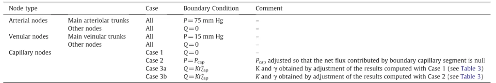
These three different conditions, prescribed at capillary nodes, define the type of interactions between the territory under study and the neighboring territories. They are summarized inTable 2and described with further detail below:
- Case 1: a zero flow condition is used. The territory under study is therefore totally independent of the neighboring territories: flux
lines are parallel to the frontier and no exchange of fluid is allowed. As a consequence, this condition minimizes the regional blood flow;
- Case 2: the pressure is assigned to a constant value (Pcap). In this case,
the methodological difficulty is due to the coupling between network geometry and flow. For example, in the case of global arteriolar vasodilations (e.g. mimicking response to hypercapnia), even if the arteriolar (input) pressure and the venular (output) pressure can be kept constant as a first approximation (because the resistance of larger upstream and downstream vessels is small compared to the resistance of intracortical vessels), it is clear that the mean pressure of the capillary bed must be affected. In order to prescribe a self-consistent value for the pressure at capillary boundary nodes, Pcap can be adjusted such that the total flow
feeding the network through the arteriolar trunks equals the total flow drained by the venular trunks. In other words, Pcapcan be
adjusted such that the net flux contributed by all the boundary capillary segments is null. As a consequence, the net flux leaving the studied brain region, through capillaries, to supply neighboring areas is exactly compensated by the net flux arriving from neighboring areas through capillaries. This is a reasonable assumption because the depth of the section is greater than the size of the Representative Elementary Volume (REV)1of the capillary bed (Lorthois and Cassot, 2010). In this case, the frontiers of the domain are iso-pressure surfaces (P= Pcap), except in the vicinity of the arterial and venous
trunks. Thus, for a first approximation, the flux lines should be perpendicular to the frontier, maximizing the exchanges of fluid with the neighboring tissue. As a consequence, this condition maximizes the regional blood flow;
- Case 3: the flow rate is related to the capillary radius by a power law: Qcap= Krcapγ, where rcapis the radius and K and γ are the
coefficients obtained from adjustment of the results of Case 1 and Case 2 (seeResultsandTable 3). Moreover, contrarily to Case 2, the flow direction (incoming or outgoing flow at the capillary node) does not result from the calculation but must also be assigned. In practice, the flow direction is chosen randomly.
α β c b a γ d γ Art. Vein. In Out In Out d 500 µm
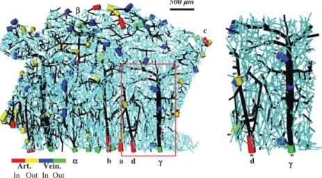
Fig. 1. Left: connectivity representation of a human microvascular network (collateral sulcus of the temporal lobe) containing 8832 nodes (including 2930 boundary nodes) and 10318 segments (including 2930 boundary segments). For clarity of representation, diameters have been increased fourfold compared to lengths. Capillary segments are displayed in light blue and non-capillary segments in black. Arteriolar and venular boundary segments are indicated by colored cylinders: the main arteriolar trunks are displayed in red whereas all other interrupted arteriolar segments are displayed in yellow; the main venular trunks are displayed in green whereas all other interrupted venular segments are in blue. Latin (resp. Greek) symbols indicate arterial (resp. venous) trunks that will be studied in more detail in the remainder of this paper). Right: Enlarged view of the area delimited by the red box in the left image, exhibiting one arteriolar and one venular intra-cortical trees. In the arteriolar tree, blood flow is from bottom (sulcus) to top (white matter): blood enters through node A1 and exits toward neighboring section through two nodes (A1*). In the venular tree, blood flow is from top (white matter) to bottom (sulcus): blood enters from neighboring section through three nodes (V1*) and is drained through the main venular trunk V1.
1In the usual sense given in the porous media literature, the scale at which a porous
In addition, the hematocrit at each input segment, i.e. boundary node with flow entering the region under study, must be prescribed in order to account for phase separation (Eq.(7)). A uniform value (Hin)
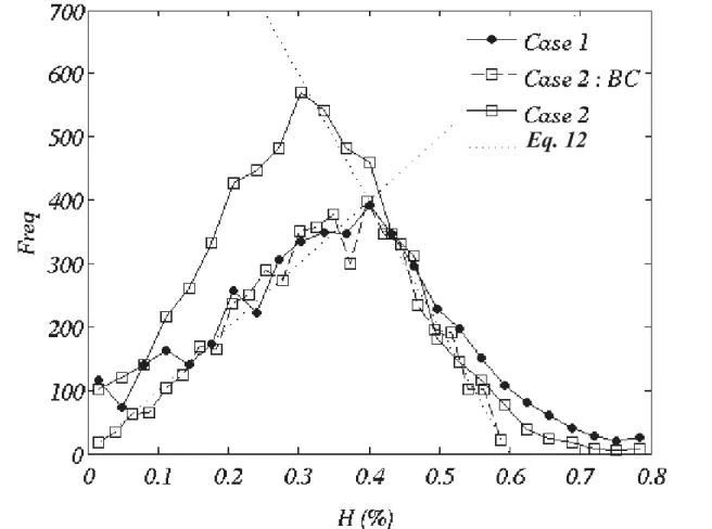
is assigned to the main arteriolar trunks. In addition, the hematocrit in capillary beds shows a large heterogeneity and its characteristic statistical distribution exhibits two linear segments and a peak around the systemic hematocrit (Pries et al., 1990). To account for this, the hematocrit of capillary nodes is randomly chosen according to the following ad-hoc normalized probability distribution function:
j
p hð Þdh = 4=
3 H! in"2 % & h if0≤h≤Hin; p hð Þdh = 8=
3 H! in"2 % & 3Hin= 2−h h i ifHinbhb3Hin= 2; p hð Þdh = 0 if3Hin= 2≤h: ð12ÞThis distribution was implemented from a uniform deviates random generator using a transformation method (Press et al., 1992). Data treatment
The computational method presented above gives the pressure at each node and the flow rate and hematocrit in each segment, i.e. a large number of data, which can be analyzed from different points of view. First, these individual data, as well as related quantities derived for each segment (velocity, mean pressure, wall shear stress, erythrocyte flow, etc) can be analyzed directly by studying their frequency distributions, spatial maps or dependence between each other (e.g. flow in each segment as a function of segment radius). Second, these data can be averaged over parallelepiped regions of interest (ROIs) of depth equal to the depth of the thick section. Averaging is performed depending on the variable under study to retain its physical significance. For example, the ROI blood flow is calculated as the total flow entering the ROI through any of its segments. The sides of the parallelepipeds in the plan of the section (250 or 500μm) is chosen such that the volume of each ROI is small compared to the entire volume of the mosaic but large enough to
contain a significant number of segments. The 500 μm voxel size corresponds to the typical spatial resolution of fMRI at 7Tesla (Yacoub et al., 2007). Finally, integrated quantities (i.e. quantities character-izing blood flow at the scale of the network, e.g. network resistivity, regional blood flow, mean transit time, network Fahraeus effect, etc.) can be calculated.
Results
Micro-vascular network
Fig. 1displays the intra-cortical network structure corresponding to mosaic M1 inCassot et al. (2006). This structure includes a total of 10318 segments and 8832 nodes. A large proportion of these nodes (~33%) corresponds to the 2930 boundary nodes. Among these boundary nodes, 42 arteriolar and 45 venular nodes were identified, including 11 main arteriolar and 12 main venular trunks.
As reducing the proportion of boundary nodes is not achievable in the short term (see Discussion), it is essential to investigate the influence of the prescribed BC on the baseline flow in the network, i.e. before studying any variations of the vessel diameters. Therefore, the question of whether it is possible to identify BC providing lower- or upper-bound limits to the network behavior is addressed in the next paragraph.
Baseline hemodynamics and influence of boundary conditions Regional blood flow
The regional blood flow can be calculated as a function of the BC prescribed, given the structure of the intra-cortical vascular network obtained from our quantitative library, the pressure drop from 75 mm Hg in feeding arterioles to 15 mm Hg in draining venules, and the inlet hematocrit Hin.Table 4displays the values obtained, expressed in ml/mn/ (100 g). It is not surprising that, whatever the BC, the regional flow increases with decreasing Hin. In addition, for a given Hin, the assigned
pressure condition (Case 2) maximizes the regional blood flow while the zero-flow condition (Case 1) minimizes the regional blood flow, as expected (seeMaterials and methods).
For Hin
= 0, the regional blood flow is well over the physiological value of 50 to 65 ml/mn/(100 g) observed in gray matter (Rostrup et al., 2000), whatever the BC. In contrast, for Hin= 0.4, the regional blood
Table 2
Summary of the prescribed boundary conditions.
Node type Case Boundary Condition Comment
Arterial nodes Main arteriolar trunks All P = 75 mm Hg –
Other nodes All Q = 0 –
Venular nodes Main veinular trunks All P = 15 mm Hg –
Other nodes All Q = 0 –
Capillary nodes Case 1 Q = 0 –
Case 2 P = Pcap Pcapadjusted so that the net flux contributed by boundary capillary segment is null
Case 3a Q = Krcapγ K andγ obtained by adjustment of the results computed with Case 1 (seeTable 3)
Case 3b Q = Krcapγ K and γ obtained by adjustment of the results computed with Case 2 (seeTable 3)
Table 3
Best fit for coefficients of power law Qcap= Krcapγ as a function of Hinand boundary
condition assigned at the interrupted capillaries (see Supplementary Material, Fig. SM1). rcapmust be expressed in micrometers for a flow rate expressed in nl/s. For
boundary condition “Case 3a,” and “Case 3b,” the value of the coefficients log(K) and γ, as obtained by adjustment of “Case 1” and “Case 2” results are between brackets. Note that they are different from the values obtained from fitting the “Case 3” results, demonstrating a significant discrepancy between the predicted and prescribed values.
Case 1 Case 2 Case 3a Case 3b log(K) γ log(K) γ log(K) γ log(K) γ Hin= 0.2 −3.58 3.31 −3.58 3.21 – – – – Hin= 0.4 −3.83 3.30 −3.48 3.19 −3.34 [−3.83] 2.69 [3.30] −3.05 [−3.48] 2.41 [3.19] Table 4
Baseline regional blood flow (ml/mn/(100 g)) as a function of Hinand boundary
condition prescribed at the interrupted capillaries (seeMaterials and methodsfor details). Note that in order to express the regional blood flow in ml/mn/(100 g), the raw results, expressed in ml/mn, have been rescaled over the volume of tissue corresponding to the region under study (1.21 mm3). A tissue density of 1.05 has
been assumed.
Case 1 Case 2 Case 3a Case 3b
Hin= 0 152.24 433.73 – –
Hin= 0.2 58.78 408.05 – –
flow calculated using the zero flow BC (Case 1) and the assigned pressure BC (Case 2) surround the physiological value, the first BC providing an underestimate and the second BC an overestimate. The assigned flow rate BC (Case 3) also, though to a lesser extent, overestimates the regional blood flow. This result is noteworthy because no adjustable parameter was used in the calculations, demonstrating the relevance of the methodology used, as well as the relevance of these three BC.
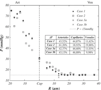
Pressure drop
The distribution of mean pressure drop among arteries, capillaries and venules as a function of their radius is displayed inFig. 2. The pressure drop is predicted to be steeper in the arterial side than in the venous side, in agreement with trends experimentally observed in other organs (Pries et al., 1990;Lipowsky, 2005; Piechnik et al., 2008). In addition, the mean value of capillary pressure (Table 5) is in reasonable accordance with the value of 34 mm Hg found byEspagno et al. (1969)
for the human brain microcirculation (cited byZagzoule and Marc-Vergnes, 1986). However, a closer examination ofFig. 2exhibits some aberrant pressure values when the assigned flow rate BC (Case 3) is used. In this case, the predicted pressure in 12μm −14 μm venular vessels (14.66 mm Hg and 12.87 mm Hg for Case 3a and 3b, respectively) is lower than the pressure assigned at the venous outlets (15 mm Hg). This underestimation may appear to be small but, when the whole pressure distribution is considered, 891 segments in Case 3a
and 1429 in Case 3b display a mid-segment pressure lower than 15 mm Hg. 307 segments in Case 3a and 421 in Case 3b even display a negative pressure (data not shown). Thus, with regard to pressure distribution, this latter BC is irrelevant.
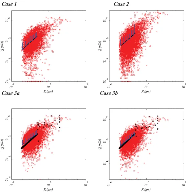
Flow rate dependence on radius in capillary vessels
Despite the very large dispersion of flow rates for a given radius (several orders of magnitude), averaged flow rates vary according to the radius following a power law Qcap= Krcapγ (see Supplementary
Material, Fig. SM1).Table 3displays the coefficients K and γ obtained by least square interpolation in the different conditions studied. For BC Case 3a and 3b, a significant discrepancy between predicted and imposed values of log(K) and γ is evidenced, once again suggesting that this latter BC is inappropriate (see legend ofTable 3for details, as well as Fig. SM1).
Conclusion on boundary conditions
Taken all together, these results suggest that the assigned flow rate boundary condition (Case 3) is inappropriate for capturing the hemodynamics of the intra-cortical network under study. On the other hand, zero flow and assigned pressure boundary conditions are relevant and respectively provide a lower- and an upper-bound for the network behavior. Furthermore, with Hin= 0.4, the predicted
regional blood flow underestimates the physiologic value (50 to 65 ml/mn/(100 g)) by a factor 1.5 to 2 (Case 2), whereas the prediction overestimates the physiologic value by a factor 3.6 to 4.7 (Case 3), i.e. in a reasonably symmetrical manner. Thus, the whole analysis which follows will be restricted to BC “Case 1” and “Case 2” with Hin= 0.4.
Hematocrit frequency distribution
The frequency distribution of discharge hematocrit in the network is shown in Fig. SM2 (see Supplementary Material). In both Case 1 and Case 2, this distribution exhibits the characteristic behavior with a peak surrounded by two quasi-linear segments, as measured byPries et al. (1990)in the rat mesenteric network. Thus, the hematocrit distribution is in qualitative agreement with the available experi-mental data.
Spatial distributions of pressure and flow
The spatial distributions of pressure and flow in the network are displayed inFig. 3. Even if, as expected, the BC used has a clear influence on the flow structure, some common features emerge. Regarding pressure maps, high pressure regions evidence the functional territories of arteries whereas low pressure regions evidence the functional territories of veins, which are conspicuously not segregated in space. However, due to the smoothing effect of the assigned pressure condition, these functional territories are slightly less extended in space in Case 2 than in Case 1. Equally, as the pressure is also assigned in several capillaries in between the territories of adjacent arterioles or venules, there is a clearer distinction between the territories of every single arteriole (venule) in Case 2. By contrast, in Case 1, the territories of adjacent arterioles are merged. Regarding flow maps, high flow segments clearly correspond to the main trunks of arteriolar and venular trees, with flow significantly decreasing in secondary vessels, and decreasing by several orders in capillaries. Of course, in Case 1, the proportion of capillary segments with zero flow (dark blue segments in
Fig. 3) is higher.
Arteriolar and venular territories
An alternative and quantitative approach for determining the vascular territories of a given arteriole is to tag the blood entering the network through the particular arteriole and to follow it (Turner, 2002). In other words, from each arteriolar trunk, all segments are tagged following pathways of positive flow rates. Equally, the blood drained by a given venule can be tagged following pathways of negative flow rates to
Cap 80 70 60 50 40 30 20 10 20 10 10 20 30 40 Case 1 Case 2 Case 3a Case 3b P = 15mmHg Art Ven
P
(mmHg)
Arterioles Capillaries Venules Case 1 43,52% 44,87% 11,62% Case 2 61,20% 18,92% 19,88% Case 3a 42,37% 46,60% 11,03% Case 3b 43,13% 46,88% 9,98% ∆P
R (µm)
Fig. 2. Mean baseline pressure as a function of vessel radius, for the different boundary conditions tested and Hin= 0.4. For arterioles and venules, pressure has been averaged
over 2μm vessel radius ranges. Mean capillary pressure has been calculated for all capillary segments, i.e. smaller than 4.95μm in radius. Note that no significant difference is observed when Hin= 0.2 (i.e., for each radius, pressure values differ by less
than 2 mm Hg, data not shown).
Table 5
Baseline mean capillary pressure (mm Hg) as a function of Hinand boundary condition
prescribed at the interrupted capillaries (seeMaterials and methodsfor details). In case of boundary condition “Case 2”, the value of the prescribed capillary pressure Pcapis
indicated between brackets. Note that it is very close to the mean capillary pressure, showing no discrepancy between the predicted and prescribed values.
Case 1 Case 2 Case 3a Case 3b Hin= 0 30.81 33.80 [34.80] – –
Hin= 0.2 31.36 32.45 [32.95] – –
identify the cortical region drained by this venule (see Fig. 4for a schematic illustration of the method). In practice, segments with an absolute flow value below a given threshold (0.2 nl/min) are not considered when determining these territories. As an example,Fig. 5
displays the spatial regions fed or drained by three distinct arteries or veins as determined using BC Case 1. From this figure, it is clear that the territories of arteries and veins are not paired. Moreover, the laminar extension of the territories is highly dependent on the vessels considered. Schematically, with regard to arterioles, two main classes can be identified: arterioles whose territory is restricted to the superficial layers of the cortex (e.g. arteriole a inFig. 5) or arterioles whose territory spans the entire depth of the cortex (e.g. arterioles b and c inFig. 5). With regard to the veins, the territory patterns are more diverse, with no obvious simple classification. However, it is noteworthy that several veins drain a very large territory (e.g. venule γ inFig. 5).
The volume of the territories can subsequently be calculated as the sum of the volumes of each of the tagged segments. As previously, the volumes of territories obtained with BC Case 2 (8.50 105 to 1.94
107μm3) are less extended than those obtained using BC Case 1 (8.90
105 to 2.36 107μm3). However, they are highly correlated, with a
Pearson's r coefficient of 0.94 and a significance level against the null hypothesis (no correlation), tested by a t-test as inSokal and Rohlf (1995), of 0.001. Their ratio, obtained by linear regression, is 0.77. Moreover, as displayed inFig. 6, the volumes of the venous territories are significantly correlated with the mean diameters of their venular trunks (r = 0.78 at a significance level of 0.01 in Case 1 and r = 0.89 at a significance level of 0.0025 in Case 2). The slope of the correlation is almost independent of the BC used (0.41 and 0.39 in Case 1 and Case 2, respectively).
Fig. 3. Spatial distributions of baseline pressure (left column) and flow rate (right column) for zero flow (Case 1) BC (first row) and assigned pressure (case 2) BC (second row) and Hin= 0.4. Numerical values of mean pressure and flow rate in each segment are color-coded as indicated in the color scale. For clarity of representation, diameters have been
increased threefold compared to lengths. In addition, due to the large dispersion of flow rates in segments of different diameters, the flow rate color scale is logarithmic. The normalized distributions corresponding to these maps are displayed in Fig. SM5.
A1 A2 V1 V2 A1 A2 V1 V2 A1 territory A2 territory V1 territory V2 territory
Fig. 4. Schematic representation of arterial (left) and venous (right) territories associated with a simplified vascular network, including two main arteriolar (A1 and A2) and two main venular (V1 and V2) trunks. Arteries, veins and capillaries are represented with black bold lines, gray bold lines and black thin lines, respectively. Flow direction is represented by arrows. A given vessel is in the arterial territory of a given arteriole if and only if it is possible to draw a path between this arteriole and this vessel, always following the flow direction. A given vessel is in the venous territory of a given venule if and only if it is possible to draw a path between this segment and the venule always, following the flow direction. Note that the intersection between the territories of the two arteries is not empty. The same is true for the intersections between the territories of the two veins.
Blood flow: correlation with vascular structure?
In order to seek for relationships between blood flow and vascular structure at baseline, two distinct approaches were adopted. First, a correlation was sought between the flow rate in each vascular trunk (arteries and veins) and the volume of their territories, determined as above. In Case 1, the Pearson's r coefficient is 0.6, indicating a weak correlation, with a significance level of 0.005. In Case 2, a stronger correlation is observed (r = 0.73 at a significance level of 0.001). These correlations can be slightly improved (see Fig. SM3, Supplementary Material) by seeking a power relationship between the variables by regression analysis in bi-logarithmic coordinates. In both cases, the Pearson's r coefficient is improved (0.65 and 0.77 in Case 1 and Case 2,
respectively) and, in Case 1, the significance level is improved to 0.0025 (unchanged in Case 2). This significance level is very good bearing in mind the small number of vascular trunks to be studied in the mosaic (n = 20). In addition, it is noteworthy that the exponent in the power relationship is independent of the BC prescribed (a = 0.46, see Fig. SM3).
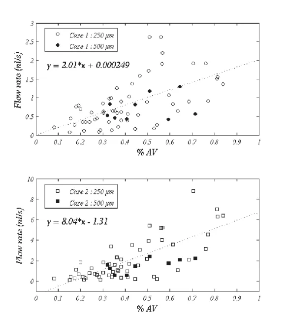
However, this approach is a “non-local” approach, because the vascular territories can span large volumes of tissue and cannot be known a priori. Thus, in addition, a correlation was also sought between flow in parallelepiped ROIs and local structural parameters represen-tative of these ROIs, such as vascular density, exchange surface or proportion of vascular space occupied by non-capillary vessels. No
Fig. 5. Spatial regions fed (respectively drained) by three distinct arteries (veins) as determined using the zero flow BC (Case 1) and Hin=0.4. Arterial territories are green and venous
territories are yellow, with vascular trunks highlighted in red and blue respectively (Symbols refer to vascular trunks as defined onFig. 1). A given arterial territory highlights a single arterial tree and its spatial relationships with its draining veins. Conversely, a given venous territory highlights a unique venous tree and its spatial relationships with its feeding arteries. As a result, these functional arterial and venous territories are not paired. This is illustrated in the figure by displaying on each line (right) the venous territory of one of the veins belonging to the territory of the artery chosen on the left.
significant correlation was found, except with the proportion of vascular space occupied by non capillary vessels (see Fig. SM4, Supplementary Material). In 250μm ROIs, this correlation is weak but significant (p b 0.001) with both boundary conditions used (Pearson's r coefficients of 0.59 and 0.74 in Case 1 and case 2, respectively (n =56)). Due to the reduced number of 500μm ROIs (n =9), no correlation can be detected in Case 1 whereas in Case 2, a Pearson's r of 0.69 at a significance level of 0.025 is obtained. In addition, as the flow rate is a flux quantity, the results obtained in both kinds of ROIs can be quantitatively compared if the flow rate in 500 μm ROIs is rescaled by a factor 6/16 to account for the difference in total surface between a single 250μm ROI and a single 500μm ROI of depth equal to the depth of the thick section. This comparison (open symbol vs. filled symbols in Fig. SM4) is satisfactory, demonstrating the relevance of the observed correlation, which is indeed independent of the size of the ROIs. This means that the architectures of the vascular tree is directly correlated to the hemodynamic pattern at voxel scale. Thus, spatial heterogeneities in CBF cannot be considered as pure noise.
Discussion
In this paper, a large and unique quantitative data library on the architecture of the microcirculation of the human cerebral cortex (Cassot et al., 2006; Lauwers et al., 2008) has been used to investigate its baseline structure/function relationship through numerical blood flow simulations. To the best of our knowledge, such simulations (large network, geometrically and topologically accurate anatomical data sets of the human cortex) have never been done before. Before discussing the results obtained about baseline flow and their implications for functional imaging, several methodological aspects, related either to the available data set or to the numerical method for blood flow simulation, will first be addressed.
Methodological aspects
The first methodological limitation of our study is due to the relatively limited thickness of the brain sections in the available data set. In fact, the large proportion (~1/3) of boundary nodes in the network is a direct consequence of the anatomical preparations used (thick sections): the volume of brain tissue investigated inCassot et al. (2006)scales as Sh, S being the total surface and h the depth of tissue scanned by confocal microscopy. If, as a rough estimate, we assume that vascular nodes are separated by a characteristic distance dc, then
the total number of boundary nodes to be found at the lower and upper surfaces of the section should scale as 2 S/dc2whereas the total
number of nodes to be found in the volume under investigation
should scale as Sh/dc3. Therefore, the proportion of boundary nodes
should scale as 2 dc/h. Here, h is about 300μm, which leads to
dc~ 50μm. This value corresponds closely with the mean capillary
length determined byCassot et al. (2006)in mosaic M1 (57.37μm) as well with the mean value of the extravascular distance (50μm), which provides an alternative definition for the order of magnitude of the capillary mesh (Cassot et al., 2006). It is also in accordance with the characteristic length of the capillary lattice determined using classic multi-scale tools (Lorthois and Cassot, 2010).
As a consequence, reducing the proportion of boundary nodes is not achievable in the short term, because it would require a new methodological framework for the acquisition of data, either using biphotonic confocal microscopy on consecutive (adjacent) brain slices and applying an alignment procedure to the subsequent linesets, or else using other material preparation techniques such as methylme-tacrilate (mercox) casting with complete tissue removal, which would allow a much deeper penetration of the laser beam.
To overcome this difficulty, which is currently unavoidable as far as human anatomical data are concerned, we have carefully investigated the influence of the capillary boundary condition over the baseline flow in the network. By this way, we have identified two different boundary conditions (zero flow and assigned pressure) which respectively provide a lower- and a upper-bound limit to the network behavior. These lower and upper limits surround the physiological values, allowing the utilization of the available data set for fluid dynamic modeling. In particular, we have demonstrated that, with regard to cerebral blood flow, these two boundary conditions respectively provide an under- and over-estimate of the physiological value. This result, obtained without any adjustable parameters (in the sense that every input variable for the model was either deduced from literature values or from the data library used), suggests that the methodology used is valid, providing quantitative results. Moreover, the slope of the correlations between the volumes of the venular territories and the mean diameter of their venular trunks, as well as the exponent of the power relationship between the volume of arterial or venous territories and the flow rate in their vascular trunks, are independent of the boundary condition used.
The second methodological limitation of the present study is intrinsic in the numerical method used for blood flow simulation, which is only able to handle steady states. This does not matter for the study of baseline flow structures. However, with regard to the flow variations induced by modifications of arteriolar diameters, the present methodology does not allow any conclusion on temporal dynamics. Nevertheless, the spatial dynamics can be explored further by focusing on flow re-organizations observed between two steady states. Baseline flow: implications for functional imaging
Several brief observations with relevance to functional imaging can be made from the study of baseline flow. First, large heterogeneities of baseline flow, not only from vessel to vessel (Fig. 3) but also from voxel to voxel (see Fig. SM4) have been demonstrated, which is consistent with earlier experimental knowledge (Pawlik et al., 1981; Kuschinsky and Paulson, 1992; Villringer et al., 1994). These voxel to voxel heterogeneities are correlated to the underlying vascular structure: the voxels with the larger proportion of arteriolar or venular vessels exhibit larger flow rates. Therefore, these heterogeneities cannot be considered as noise. Of course, they increase with decreasing voxel size. Thus, they might turn out to be of importance, especially in the context of high field imaging, where voxel size approaches the minimal size studied in the present work (250μm), and in studies focused on signal fluctuations in the absence of stimuli (e.g. during sleep,Fukunaga et al., 2008).
Second, our results suggest that regional blood flow at ROI level scales with the surface of the ROI and not its volume (see Fig. SM4). Thus, the usual normalization of regional blood flow with mass or
Fig. 6. Volume (V) of venous territories as a function of diameter of their vascular trunks (D). Circles and plain line: Case 1; Squares and dotted line: Case 2. Hin= 0.4.
volume, and the corresponding unit traditionally used for cerebral blood flow (expressed in ml/min/100 g), might be misleading.
Finally, our data on baseline flow can be used to estimate the extent of venous contamination downstream to the sites of neuronal activation. Orders of magnitude have previously been presented by
Turner (2002)for pial veins on the basis of structural data obtained from photomicrographs of the cortical surface, and considering only a single venular tree. This analysis led to the following cubic relationship between the catchment surface of an activated area D (expressed in mm2) and the diameter d
vof the single vein draining
this area (expressed in mm):
D = 520d3v: ð13Þ
From our flow data, the volume V of the territories drained by the cortical veins have been calculated, demonstrating a linear dependence with the diameter of the draining vein, with slope independent of the Boundary Condition used (seeFig. 6). If, following Turner, reasonable values for the cortical thickness t (3 mm) and blood volume fraction β in the gray matter (2%) are used, D can be estimated by V/(tβ), leading to:
D = 6:66dv: ð14Þ
In the above expression, D is expressed in mm2and d
vin mm. The
intercept, which is less than 0.05 in dimensional form with both Boundary Conditions used, has been neglected. Thus, for intra-cortical veins, a linear relationship instead of a cubic one is demonstrated. It is interesting to note that both expressions predict the same catchment areas (0.75 mm2) for veins of 113μm diameter, i.e. roughly at transition between pial and intra-cortical vasculature. Below, i.e. for the physiological range of intraintra-cortical veins, the cortical area drained by a single vein would be underestimated if Eq.(13)was used: for example, D predicted by this equation is 5 times lower than D predicted by Eq.(14)in 50μm veins. Thus, despite the generality of Turner's model, it is not possible to extrapolate its cubic expression to intracortical veins, including principal intracortical veins. This result might be of importance in the context of high field imaging.
Of course, in functional neuroimaging, two different states–an activated state and a reference state–are compared. Thus, the flow re-organizations in response to modifications of arteriolar diameters, as well as their implications for functional imaging, are explored further in a companion paper (Lorthois et al., 2010).
Supplementary materials related to this article can be found online atdoi:10.1016/j.neuroimage.2010.09.032.
Acknowledgments
Kamil Uludağ must be thanked for useful discussions. We gratefully acknowledge the anonymous referees for their constructive comments and suggestions. We also thank Victoria McBride who considerably helped to improve the English of this manuscript. This work has been partly supported by ACI Technologies pour la Santé Grant Number 02TS031 of the French Department of Education, Research and Technology and by GDR CNRS 2760 “Biomécanique des fluides et des transferts: Interactions Fluide Structure Biologique”. References
Ances, B.M., Leontiev, O., Perthen, J.E., Liang, C., Lansing, A.E., Buxton, R.B., 2008. Regional differences in the coupling of cerebral blood flow and oxygen metabolism changes in response to activation: implications for BOLD-fMRI. Neuroimage 39, 1510–1521.
Aubert, A., Costalat, R., 2002. A model of the coupling between brain electrical activity, metabolism, and hemodynamics: application to the interpretation of functional neuroimaging. Neuroimage 17, 1162–1181.
Baskurt, O.K., Farley, R.A., Meiselman, H.J., 1997. Erythrocyte aggregation tendency and cellular properties in horse, human, and rat: a comparative study. Am. J. Physiol. 273, H2604–H2612.
Bear, J., 1972. Dynamics of fluids in porous media. American Elsevier Publishing Company, New York.
Boas, D.A., Jones, S.R., Devor, A., Huppert, T.J., Dale, A.M., 2008. A vascular anatomical network model of the spatio-temporal response to brain activation. Neuroimage 40, 1116–1129.
Buxton, R.B., Wong, E.C., Frank, L.R., 1998. Dynamics of blood flow and oxygenation changes during brain activation: the Balloon model. Magn. Reson. Med. 39, 855–864. Buxton, R.B., Uludağ, K., Dubowitz, D.J., Liu, T.T., 2004. Modeling the hemodynamic
response to brain activation. Neuroimage 23, S220–S233.
Cassot, F., Lauwers, F., Fouard, C., Prohaska, S., Lauwers-Cances, V., 2006. A novel three-dimensional computer-assisted method for a quantitative study of microvascular networks of the human cerebral cortex. Microcirculation 13, 1–18.
Cassot, F., Lauwers, F., Lorthois, S., Puwanarajah, P., Duvernoy, H., 2009. Scaling laws for branching vessels of human cerebral cortex. Microcirculation 16, 331–344. Cox, S.B., Woolsey, T.A., Rovainen, C.M., 1993. Localized dynamic changes in cortical
blood flow with whisker stimulation corresponds to matched vascular and neuronal architecture of rat barrels. J. Cereb. Blood Flow Metab. 13, 899–913. Davis, T.L., Kwong, K.K., Weisskoff, R.M., Rosen, B.R., 1998. Calibrated functional MRI: mapping
the dynamics of oxidative metabolism. Proc. Natl. Acad. Sci. USA 95, 1834–1839. D'Esposito, M., Deouell, L.Y., Gazzaley, A., 2003. Alterations in the BOLD fMRI signal with
ageing and disease: a challenge for neuroimaging. Nat. Rev. Neurosci. 4, 863–872. Devor, A., Tian, P., Nishimura, N., Teng, I.C., Hillman, E.M., Narayanan, S.N., Ulbert, I., Boas, D.A., Kleinfeld, D., Dale, A.M., 2007. Suppressed neuronal activity and concurrent arteriolar vasoconstriction may explain negative blood oxygenation level-dependent signal. J. Neurosci. 27, 4452–4459.
Duong, T.Q., Kim, D.S., Ugurbil, K., Kim, S.G., 2001. Localized cerebral blood flow response at submillimeter columnar resolution. Proc. Natl. Acad. Sci. USA 98, 10904–10909. Duvernoy, H.M., Delon, S., Vannson, J.L., 1981. Cortical blood vessels of the human brain.
Brain Res. Bull. 7, 519–579.
Espagno, J., Arbus, L., Bes, A., Billet, R., Gouaze, A., Frerebeau, Ph., Lazorthes, Y., Salamon, G., Seylaz, J., Vlahovitch, B., 1969. La circulation cérébrale. Neuro-Chirurgie 15, Suppl. 2.
Fang, Q., Sakadzic, S., Ruvinskaya, L., Devor, A., Dale, A., Boas, D.A., 2008. Oxygen advection and diffusion in a three dimensional vascular anatomical network. Opt. Express 16, 17530–17541.
Fouard, C., Malandain, G., Prohaska, S., Westerhoff, M., 2006. Blockwise processing applied to brain microvascular network study. IEEE Trans. Med. Imaging 25, 1319–1328. Fukunaga, M., Horovitz, S.G., de Zwart, J.A., van Gelderen, P., Blakin, T.J., Braun, A.R.,
Duyn, J.H., 2008. Metabolic origin of BOLD signal fluctuations in the absence of stimuli. J. Cereb. Blood Flow Metab. 28, 1377–1387.
Fung, Y.C., 1996. Biomechanics: circulation. Springer, New York.
Gaehtgens, P., 1992. Why networks ? Int. J. Microcirc. Clin. Exp. 11, 123–133. Harel, N., Ugurbil, K., Uludag, K., Yacoub, E., 2006. Frontiers of brain mapping using MRI.
J. Magn. Reson. Imaging 23, 945–957.
Harrison, R.V., Harel, N., Panesar, J., Mount, R.J., 2002. Blood capillary distribution correlates with hemodynamic-based functional imaging in cerebral cortex. Cereb. Cortex 12, 225–233.
Heinzer, S., Krucker, T., Stampanoni, M., Abela, R., Meyer, E.P., Schuler, A., Schneider, P., Müller, R., 2006. Hierarchical microimaging for multiscale analysis of large vascular networks. Neuroimage 32, 626–636.
Klein, B., Kuschinsky, W., Schröck, H., Vetterlein, F., 1986. Interdependency of local capillary density, blood flow, and metabolism in rat brains. Am. J. Physiol. 251, H1333–H13340. Kuschinsky, W., Paulson, O.B., 1992. Capillary circulation in the brain. Cerebrovasc.
Brain Metab. Rev. 4, 261–286.
Lauwers, F., Cassot, F., Lauwers-Cances, V., Puwanarajah, P., Duvernoy, H., 2008. Morphometry of the human cerebral cortex microcirculation: general characteristics and space-related profiles. Neuroimage 39, 936–948.
Lipowsky, H.H., 2005. Microvascular rheology and hemodynamics. Microcirculation 12, 5–15. Logothetis, N.K., 2008. What we can do and what we cannot do with fMRI. Nature 453,
869–878.
Logothetis, N.K., Wandell, B.A., 2004. Interpreting the BOLD signal. Annu. Rev. Physiol. 66, 735–769.
Lorthois, S., Cassot, F., 2010. Fractal analysis of vascular networks: insights from morphogenesis. J. Theor. Biol. 262, 614–633.
Lorthois, S., Cassot, F., Lauwers, F., 2010. Simulation study of brain blood flow regulation by intra-cortical arterioles in an anatomically accurate large human vascular network. Part II: Flow variations induced by global or localized modifications of arteriolar diameters. Neuroimage.doi:10.1016/j.neuroimage.2010.10.040
.
Mandeville, J.B., Marota, J.J., Ayata, C., Zaharchuk, G., Moskowitz, M.A., Rosen, B.R., Weisskoff, R.M., 1999. Evidence of a cerebrovascular postarteriole windkessel with delayed compliance. J. Cereb. Blood Flow Metab. 19, 679–689.
Paulson, O.B., 2002. Blood-brain barrier, brain metabolism and cerebral blood flow. Eur. Neuropsychopharmacol. 12, 495–501.
Pawlik, G., Rackl, A., Bing, R.J., 1981. Quantitative capillary topography and blood flow in the cerebral cortex of cats: an in vivo microscopic study. Brain Res. 208, 35–58. Piechnik, S.K., Chiarelli, P.A., Jezzard, P., 2008. Modeling vascular reactivity to
investigate the basis of the relationship between cerebral blood volume and flow under CO2 manipulation. Neuroimage 39, 107–118.
Press, W.H., Flannery, B.P., Teukolsky, S.A., Vetterling, W.T., 1992. Numerical Recipes. C: The Art of Scientific Computing. Cambridge University Press.
Pries, A.R., Ley, K., Claassen, M., Gaehtgens, P., 1989. Red cell distribution at microvascular bifurcations. Microvasc. Res. 38, 81–101.
Pries, A.R., Secomb, T.W., Gaehtgens, P., Gross, J.F., 1990. Blood flow in microvascular networks. Experiments and simulation. Circ. Res. 67, 826–834.
Pries, A.R., Secomb, T.W., Gaehtgens, P., 1996. Biophysical aspects of blood flow in the microvasculature. Cardiovasc. Res. 32, 654–667.
Pries, A.R., Reglin, B., Secomb, T.W., 2003. Structural response of microcirculatory networks to changes in demand: information transfer by shear stress. Am. J. Physiol. Heart Circ. Physiol. 284, H2204–H2212.
Reichold, J., Stampanoni, M., Keller, A.L., Buck, A., Jenny, P., Weber, B., 2009. Vascular graph model to simulate the cerebral blood flow in realistic vascular networks. J. Cereb. Blood Flow Metab. 29, 1429–1443.
Reina-De La Torre, F., Rodriguez-Baeza, A., Sahuquillo-Barris, J., 1998. Morphological characteristics and distribution pattern of the arterial vessels in human cerebral cortex: a scanning electron microscope study. Anat. Rec. 251, 87–96.
Risser, L., Plouraboué, F., Steyer, A., Cloetens, P., Le Duc, G., Fonta, C., 2007. From homogeneous to fractal normal and tumorous microvascular networks in the brain. J. Cereb. Blood Flow Metab. 27, 293–303.
Rostrup, E., Law, I., Blinkenberg, M., Larsson, H.B., Born, A.P., Holm, S., Paulson, O.B., 2000. Regional differences in the CBF and BOLD responses to hypercapnia: a combined PET and fMRI study. Neuroimage 11, 87–97.
Secomb, T.W., Hsu, R., Beamer, N.B., Coull, B.M., 2000. Theoretical simulation of oxygen transport to brain by networks of microvessels: effects of oxygen supply and demand on tissue hypoxia. Microcirculation 7, 237–247.
Secomb, T.W., Hsu, R., Park, E.Y., Dewhirst, M.W., 2004. Green's function methods for analysis of oxygen delivery to tissue by microvascular networks. Ann. Biomed. Eng. 32, 1519–1529.
Shmuel, A., Yacoub, E., Pfeuffer, J., Van de Moortele, P.F., Adriany, G., Hu, X., Ugurbil, K., 2002. Sustained negative BOLD, blood flow and oxygen consumption response and its coupling to the positive response in the human brain. Neuron 36, 1195–1210.
Sokal, R.R., Rohlf, F.J., 1995. Biometry, Third Edition. WH freeman and Co., New York.
Turner, R., 2002. How much cortex can a vein drain? Downstream dilution of activation-related cerebral blood oxygenation changes. Neuroimage 16, 1062–1067. Uludağ, K., Müller-Bierl, B., Uğurbil, K., 2009. An integrative model for neuronal
activity-induced signal changes for gradient and spin echo functional imaging. Neuroimage 48, 150–165.
Valabrègue, R., Aubert, A., Burger, J., Bittoun, J., Costalat, R., 2003. Relation between cerebral blood flow and metabolism explained by a model of oxygen exchange. J. Cereb. Blood Flow Metab. 23, 536–545.
Villringer, A., Them, A., Lindauer, U., Einhäupl, K., Dirnagl, U., 1994. Capillary perfusion of the rat brain cortex: an in vivo confocal microscopy study. Circ. Res. 75, 55–62. Weber, B., Keller, A.L., Reichold, J., Logothetis, N.K., 2008. The microvascular system of the striate and extrastriate visual cortex of the macaque. Cereb. Cortex 18, 2318–2330. Weisstein, E.W., 1998. CRC concise encyclopedia of mathematics. CRC Press. Woolsey, T.A., Rovainen, C.M., Cox, S.B., Henegar, M.H., Liang, G.E., Liu, D., Moskalenko,
Y.E., Sui, J., Wei, L., 1996. Neuronal units linked to microvascular modules in cerebral cortex: response elements for imaging the brain. Cereb. Cortex 6, 647–660. Yacoub, E., Shmuel, A., Logothetis, N., Ugurbil, K., 2007. Robust detection of ocular dominance columns in humans using Hahn Spin Echo BOLD functional MRI at 7 Tesla. Neuroimage 37, 1161–1177.
Zagzoule, M., Marc-Vergnes, J.P., 1986. A global mathematical model of the cerebral circulation in man. J. Biomech. 19, 1015–1022.
Zheng, Y., Mayhew, J., 2009. A time-invariant visco-elastic windkessel model relating blood flow and blood volume. Neuroimage 47, 1371–1380.
Zheng, Y., Martindale, J., Johnston, D., Jones, M., Berwick, J., Mayhew, J., 2002. A model of the hemodynamic response and oxygen delivery to brain. Neuroimage 16, 617–637.