Application of a multimodel approach to account for conceptual model and scenario 1
uncertainties in groundwater modelling 2
3
Rodrigo Rojas*a,1, Samalie Kahundeb, Luk Peetersa, Okke Batelaana,c , Luc Feyend, and Alain 4 Dassarguesa,e 5 6 * Corresponding author 7
a Applied geology and mineralogy, Department of Earth and Environmental Sciences, 8
Katholieke Universiteit Leuven. Celestijnenlaan 200E, B-3001 Heverlee, Belgium. Tel.: + 32 9
016 326449, Fax: + 32 016 326401. 10
E-mail address: [email protected]
11
E-mail address: [email protected]
12 13
b Interuniversity Programme in Water Resources Engineering (IUPWARE), Katholieke 14
Universiteit Leuven and Vrije Universiteit Brussel. Pleinlaan 2, B-1050 Brussels, Belgium. 15
Tel: + 32 2 6293039, Fax: + 32 2 6293022. 16
E-mail address: [email protected]
17 18
c Department of Hydrology and Hydraulic Engineering, Vrije Universiteit Brussel. Pleinlaan 19
2, B-1050 Brussels, Belgium. Tel: + 32 2 6293039, Fax: + 32 2 6293022. 20
E-mail address: [email protected]
21 22
d Land management and natural hazards unit, Institute for Environment and Sustainability 23
(IES), DG- Joint Research Centre (JRC), European Commission (EC). 24
Via Enrico Fermi 2749, TP261, I-21027, Ispra (Va), Italy. 25
Tel: +39 0332789258, Fax: +39 0332 786653 26
E-mail address: [email protected] 27
28
e Hydrogeology and Environmental Geology, Department of Architecture, Geology, 29
Environment, and Constructions (ArGEnCo), Université de Liège. B.52/3 Sart-Tilman, B-30
4000 Liège, Belgium. Tel.: + 32 4 3662376, Fax: + 32 4 3669520. 31
E-mail address: [email protected]
32 33 34
1 Now at: Land management and natural hazards unit, Institute for Environment and 35
Sustainability (IES), DG- Joint Research Centre (JRC), European Commission (EC). 36
Via Enrico Fermi 2749, TP261, I-21027, Ispra (Va), Italy. 37
Tel: +39 0332 78 97 13, Fax: +39 0332 78 66 53 38
E-mail address: [email protected] 39
40 41 42
Manuscript submitted to Journal of Hydrology on September 2nd , 2009 43
* Revised manuscript HYDROL7809
Abstract 1
Groundwater models are often used to predict the future behaviour of groundwater systems. 2
These models may vary in complexity from simplified system conceptualizations to more 3
intricate versions. It has been recently suggested that uncertainties in model predictions are 4
largely dominated by uncertainties arising from the definition of alternative conceptual 5
models. Different external factors such as climatic conditions or groundwater abstraction 6
policies, on the other hand, may also play an important role. Rojas et al. (2008) proposed a 7
multimodel approach to account for predictive uncertainty arising from forcing data (inputs), 8
parameters, and alternative conceptualizations. In this work we extend upon this approach to 9
include uncertainties arising from the definition of alternative future scenarios and we 10
improve the methodology by including a Markov Chain Monte Carlo sampling scheme. We 11
apply the improved methodology to a real aquifer system underlying the Walenbos Nature 12
Reserve area in Belgium. Three alternative conceptual models comprising different levels of 13
geological knowledge are considered. Additionally, three recharge settings (scenarios) are 14
proposed to evaluate recharge uncertainties. A joint estimation of the predictive uncertainty 15
including parameter, conceptual model, and scenario uncertainties is estimated for 16
groundwater budget terms. Finally, results obtained using the improved approach are 17
compared with the results obtained from methodologies that include a calibration step and 18
which use a model selection criterion to discriminate between alternative conceptualizations. 19
Results showed that conceptual model and scenario uncertainties significantly contribute to 20
the predictive variance for some budget terms. Besides, conceptual model uncertainties played 21
an important role even for the case when a model was preferred over the others. Predictive 22
distributions showed to be considerably different in shape, central moment, and spread among 23
alternative conceptualizations and scenarios analyzed. This reaffirms the idea that relying on a 24
single conceptual model driven by a particular scenario, will likely produce bias and under-25
dispersive estimations of the predictive uncertainty. Multimodel methodologies based on the 26
use of model selection criteria produced ambiguous results. In the frame of a multimodel 27
approach, these inconsistencies are critical and can not be neglected. These results strongly 28
advocate the idea of addressing conceptual model uncertainty in groundwater modeling 29
practice. Additionally, considering alternative future recharge uncertainties will permit to 30
obtain more realistic and, possibly, more reliable estimations of the predictive uncertainty. 31
Keywords 1
Groundwater flow modelling, conceptual model uncertainty, scenario uncertainty, GLUE, 2
Bayesian Model Averaging, Markov Chain Monte Carlo. 3
4
1. Introduction and scope 5
Groundwater models are often used to predict the behaviour of groundwater systems under 6
future stress conditions. These models may vary in the level of complexity from simplified 7
groundwater system representations to more elaborated models accounting for detailed 8
descriptions of the main processes and geological properties of the groundwater system. 9
Whether to postulate simplified or complex/elaborated models for solving a given problem 10
has been subject of discussion for several years (Gómez-Hernández, 2006; Hill, 2006; 11
Neuman and Wierenga, 2003). Parsimony is the main argument for those in favour of simpler 12
models (see e.g. Hill and Tiedeman, 2007) whereas a more realistic representation of the 13
unknown true system (see e.g. Rubin, 2003; Renard, 2007) seems the main argument 14
favouring more elaborated models. To some extent, this debate has contributed to the growing 15
tendency among hydrologists of postulating alternative conceptual models to represent 16
optional dynamics explaining the flow and solute transport in a given groundwater system 17
(Harrar et al., 2003; Meyer et al., 2004; Højberg and Refsgaard, 2005; Troldborg et al., 2007; 18
Seifert et al., 2008). 19
20
It has been recently suggested that uncertainties in groundwater model predictions are largely 21
dominated by uncertainty arising from the definition of alternative conceptual models and that 22
parametric uncertainty solely does not allow compensating for conceptual model uncertainty 23
(Bredehoeft, 2003; Neuman, 2003; Neuman and Wierenga, 2003; Ye et al., 2004; Bredehoeft, 24
2005; Højberg and Refsgaard, 2005; Poeter and Anderson, 2005; Refsgaard et al., 2006; 25
Meyer et al., 2007; Refsgaard et al., 2007; Seifert et al., 2008; Rojas et al., 2008). 26
Additionally, this last situation is exacerbated for the case when predicted variables are not 27
included in the data used for calibration (Højberg and Refsgaard, 2005; Troldborg et al., 28
2007). This suggests that it is more appropriate to postulate alternative conceptual models and 29
analyze the combined multimodel predictive uncertainty than relying on a single hydrological 30
conceptual model. Working with a single conceptualization is more likely to produce biased 31
and under-dispersive uncertainty estimations whereas working with a multimodel approach, 32
uncertainty estimations are less (artificially) conservative and they are more likely to capture 33
the unknown true predicted value. 34
1
Practice suggests, however, that once a conceptual model is successfully calibrated and 2
validated, for example, following the method described by Hassan (2004), its results are 3
rarely questioned and the conceptual model is assumed to be correct. As a consequence, the 4
conceptual model is only revisited when sufficient data have been collected to perform a post-5
audit analysis (Anderson and Woessner, 1992), which often may take several years, or when 6
new collected data and/or scientific evidence challenge the definition of the original 7
conceptualization (Bredehoeft, 2005). In this regard, Bredehoeft (2005) presents a series of 8
examples where unforeseen elements or the collection of new data challenged well 9
established conceptual models. This situation clearly states the gap between practitioners and 10
the scientific community in addressing predictive uncertainty estimations in groundwater 11
modelling in presence of conceptual model uncertainty. 12
13
Different external factors such as climatic conditions or groundwater abstraction policies, on 14
the other hand, increase the uncertainty in groundwater model predictions due to unknown 15
future conditions. This source of uncertainty has since long been recognized as an important 16
source of predictive uncertainty, however, practical applications mainly focus on uncertainty 17
derived from parameters and inputs (forcing data), neglecting conceptual model and scenario 18
uncertainties (Rubin, 2003; Gaganis and Smith, 2006). Recently, Rojas and Dassargues 19
(2007) analyzed the groundwater balance of a regional aquifer in northern Chile considering 20
different projected groundwater abstraction policies in combination with stochastic 21
groundwater recharge values. Meyer et al. (2007) presented a combined estimation of 22
conceptual model and scenario uncertainties in the framework of Maximum Likelihood 23
Bayesian Model Averaging (MLBMA) (Neuman, 2003) for a groundwater flow and transport 24
modelling study case. 25
26
In recent years, several methodologies to account for uncertainties arising from inputs 27
(forcing data), parameters and the definition of alternative conceptual models have been 28
proposed in the literature (Beven and Binley, 1992; Neuman, 2003; Poeter and Anderson, 29
2005; Refsgaard et al., 2006; Ajami et al., 2007; Rojas et al., 2008). Two appealing 30
methodologies in the case of groundwater modelling are the MLBMA method (Neuman, 31
2003) and the information-theoretic based method of Poeter and Anderson (2005). Both 32
methodologies are based on the use of a model selection criterion, which is derived as a by-33
product of traditional calibration methods such as maximum likelihood or weighted least 34
squares. The use of a model selection criterion allows ranking alternative conceptual models, 1
eliminating some of them, or weighing and averaging model predictions in a multimodel 2
framework. In our case, we are interested in weighing and averaging predictions from 3
alternative conceptual models to obtain a combined estimation of the predictive uncertainty. 4
The most commonly used model selection criteria correspond to Akaike Information Criterion 5
(AIC) (Akaike, 1974), modified Akaike Information Criterion (AICc) (Hurvich and Tsai, 6
1989), Bayesian Information Criterion (BIC) (Schwartz, 1978) and Kashyap Information 7
Criterion (KIC) (Kashyap, 1982). Ye et al. (2008a) gives an excellent discussion on the merits 8
and demerits of alternative model selection criteria in the context of variogram multimodel 9
analysis. In MLBMA, KIC is the suggested criterion whereas for the information-theoretic 10
based method of Poeter and Anderson (2005), AICc is preferred. Even though Ye et al. 11
(2008a) appear to have settled the controversy on the use of alternative model selection 12
criteria, the use of different model selection criteria to weigh and combine multimodel 13
predictions in groundwater modelling may lead to controversial and misleading results. 14
15
Apart from common problems of parameter non-uniqueness (insensitivity) and ‘locality 16
behaviour’ of the calibration approaches mentioned above, Refsgaard et al. (2006) pointed out 17
an important disadvantage of including a calibration stage in a multimodel framework. In the 18
case of multimodel approaches including a calibration step, errors in the conceptual models 19
(which per definition can not be excluded) will be compensated by biased parameter estimates 20
in order to optimize model fit in the calibration stage. This has been confirmed by Troldborg 21
et al. (2007) for a real aquifer system in Denmark. 22
23
Recently, Rojas et al. (2008) proposed an alternative methodology to account for predictive 24
uncertainty arising from inputs (forcing data), parameters and the definition of alternative 25
conceptual models. This method combines the Generalized Likelihood Uncertainty 26
Estimation (GLUE) method (Beven and Binley, 1992) and Bayesian Model Averaging 27
(BMA) (Draper, 1995; Kass and Raftery, 1995; Hoeting et al., 1999). The basic idea behind 28
this methodology is the concept of equifinality, that is, many alternative conceptual models 29
together with many alternative parameter sets will produce equally likely good results when 30
compared to observed data (Beven and Freer, 2001; Beven, 2006). Equifinality, as defined by 31
Beven (1993, 2006), arises because of the combined effects of errors in the forcing data, 32
system conceptualization, measurements and parameter estimates. In the method of Rojas et 33
al. (2008) series of “behavioural” parameters are selected for each alternative model 34
producing a cumulative density function (cdf) for parameters and variables of interest. Using 1
the performance values obtained from GLUE, weights for each conceptual model are 2
estimated, and results obtained for each model are combined following BMA in a multimodel 3
frame. An important aspect of the method is that it does not rely on a unique parameter 4
optimum or conceptual model to assess the joint predictive uncertainty, thus, avoiding 5
compensation of conceptual model errors due to biased parameter estimates. A complete 6
description of the methodology and potential advantages are discussed in Rojas et al. (2008). 7
8
Rojas et al. (2008) used a traditional Latin Hypercube Sampling (LHS) scheme (McKay et al., 9
1979) to implement the combined GLUE-BMA methodology. This sampling scheme has been 10
regularly used in GLUE applications. Blasone et al. (2008a, 2008b) demonstrated that the 11
efficiency of the GLUE methodology can be boosted up by including a Markov Chain Monte 12
Carlo (MCMC) sampling scheme. MCMC is a sampling technique that produces a Markov 13
Chain with stationary probability distribution equal to a desired distribution through iterative 14
Monte Carlo simulation. This technique is particularly suitable in Bayesian inference when 15
the analytical forms of posterior distributions are not available or in cases of high dimensional 16
posterior distributions. 17
18
In this work we extend upon the methodology of Rojas et al. (2008) to include the uncertainty 19
in groundwater model predictions due to the definition of alternative conceptual models and 20
alternative recharge settings. For that, we follow an approach similar to that described in 21
Meyer et al. (2007) and patterned after Draper (1995). Additionally, we improve on the 22
sampling scheme of the combined GLUE-BMA methodology by implementing an MCMC 23
sampling scheme. We apply the improved methodology to a real aquifer system underlying 24
and feeding the Walenbos Nature Reserve area in Belgium (Fig. 1). We postulate three 25
alternative conceptual models comprising different levels of geological knowledge for the 26
groundwater system. Average recharge conditions are used to calibrate each conceptual model 27
under steady-state conditions. Two additional recharge settings corresponding to ± 2 standard 28
deviations from average recharge conditions are proposed to evaluate the uncertainty in the 29
results due to the definition of alternative recharge values. A combined estimation of the 30
predictive uncertainty including parameter, conceptual model, and scenario uncertainties is 31
estimated for a set of groundwater budget terms such as river gains and river losses, drain 32
outflows, and groundwater inflows and outflows from the Walenbos area. Finally, results 33
obtained using the combined GLUE-BMA methodology are compared with the results 34
obtained using multimodel methodologies that include a calibration step and a model 1
selection criterion to discriminate between models. 2
3
The remainder of this paper is organized as follows. In section 2, we provide a condensed 4
overview of GLUE, BMA and MCMC theory followed by a description of the procedure to 5
integrate these methods. Section 3 details the study area where the integrated uncertainty 6
assessment methodology is applied. Implementation details such as the different 7
conceptualizations, recharge uncertainties and the summary of the modelling procedure are 8
described in section 4. Results are discussed in section 5 and a summary of conclusions is 9
presented in section 6. 10
11
2. Material and methods 12
Sections 2.1, 2.2 and 2.3 elaborate on the basis of GLUE, BMA, and MCMC methodologies, 13
respectively, for more details the reader is referred to Rojas et al. (2008, 2009). 14
15
2.1. Generalized likelihood uncertainty estimation (GLUE) methodology 16
GLUE is a Monte Carlo simulation technique based on the concept of equifinality (Beven and 17
Freer, 2001). It rejects the idea of a single correct representation of a system in favour of 18
many acceptable system representations (Beven, 2006). For each potential system simulator, 19
sampled from a prior set of possible system representations, a likelihood measure (e.g. 20
gaussian, trapezoidal, model efficiency, inverse error variance, etc.) is calculated, which 21
reflects its ability to simulate the system responses, given the available observed dataset D. 22
Simulators that perform below a subjectively defined rejection criterion are discarded from 23
further analysis and likelihood measures of retained simulators are rescaled so as to render the 24
cumulative likelihood equal to 1. Ensemble predictions are based on the predictions of the 25
retained set of simulators, weighted by their respective rescaled likelihood. 26
27
Likelihood measures used in GLUE must be seen in a much wider sense than the formal 28
likelihood functions used in traditional statistical estimation theory (Binley and Beven, 2003). 29
These likelihoods are a measure of the ability of a simulator to reproduce a given set of 30
observed data, therefore, they represent an expression of belief in the predictions of that 31
particular simulator rather than a formal definition of probability. However, GLUE is fully 32
coherent with a formal Bayesian approach when the use of a classical likelihood function is 33
justifiable (Romanowicz et al., 1994). 34
1
Rojas et al. (2008) observed no significant differences in the estimation of posterior model 2
probabilities, predictive capacity and conceptual model uncertainty when a Gaussian, a model 3
efficiency or a Fuzzy-type likelihood function was used. The analysis in this work is therefore 4
confined to a Gaussian likelihood function L
(
Μ θ Y D , where Mk, ,l m)
k is the k-th conceptual 5model (or model structure) included in the finite and discrete ensemble of alternative 6
conceptualizations Μ , θ is the l-th parameter vector, l Y is the m-th input data vector, and m 7
D is the observed system variable vector. 8
9
2.2. Bayesian model averaging (BMA) 10
BMA provides a coherent framework for combining predictions from multiple competing 11
conceptual models to attain a more realistic and reliable description of the predictive 12
uncertainty. It is a statistical procedure that infers average predictions by weighing individual 13
predictions from competing models based on their relative skill, with predictions from better 14
performing models receiving higher weights than those of worse performing models. BMA 15
avoids having to choose a model over the others, instead, observed dataset D give the 16
competing models different weights (Wasserman, 2000). 17
18
Following the notation of Hoeting et al. (1999), if Δ is a quantity to be predicted, the full 19
BMA predictive distribution of Δ for a set of alternative conceptual models 20
(
M ,M ,...,M ,...,M1 2 k K)
=
Μ under different scenarios S=
(
S ,S ,...,S ,...,S1 2 i I)
is given by 21 Draper (1995) 22 23(
)
(
) (
) ( )
1 1 | I K | ,M ,Sk i M | ,Sk i Si i k p p p p = = Δ D =∑∑
Δ D D (1) 24 25Equation 1 is an average of the posterior distributions of Δ under each alternative conceptual 26
model and scenarios considered,p
(
Δ D| ,M ,Sk i)
, weighted by their posterior model 27probability, p
(
M | ,Sk D i)
, and by scenario probabilities, p( )
Si . The posterior model 28probabilities conditional on a given scenario reflect how well model k fits the observed 29
dataset D and can be computed using Bayes’ rule 30
(
)
(
) (
)
(
) (
)
=1 | M M | S M | ,S | M M | S k k i k i K l l i l p p p p p =∑
D D D (2) 1 2where p
(
M | Sk i)
is the prior probability of model k under scenario i, and p(
DMk)
is the 3integrated likelihood of the model k. An important assumption in the estimation of posterior 4
model probabilities (equation 2) is the fact that the dataset D is independent of future 5
scenarios. That is, the probability of observing the dataset D is not affected by the occurrence 6
of any future scenario Si (Meyer et al., 2007). In a strict sense, however, model likelihoods 7
may depend on future scenarios given the correlation of recharge and hydraulic conductivity. 8
Accounting for this dependency would make difficult to clearly assess the intrinsic value of 9
the conceptual models or the “extra worth” of the data itself to explain the observed system 10
responses. This assessment is beyond the scope of this article and for the sake of clarity the 11
assumption of independence of D and, as consequence, of model likelihoods and posterior 12
model probabilities from the future scenarios will be retained. 13
14
As a result, model likelihoods do not depend on the scenarios and, in contrast, prior model 15
probabilities may be a function of future scenarios. 16
17
The leading moments of the full BMA prediction of Δ are given by Draper (1995) 18 19
[
]
[
]
(
) ( )
1 1 | I K | ,M ,Sk i M | ,Sk i Si i k E E p p = = Δ D =∑∑
Δ D D (3) 20 21[
]
[
]
(
) ( )
[
] [
]
(
)
(
) ( )
[
] [
]
(
)
( )
1 1 2 1 1 2 1 | | ,M ,S M | ,S S (I) | ,M ,S | ,S M | ,S S (II) | ,S | S (III) I K k i k i i i k I K k i i k i i i k I i i i Var Var p p E E p p E E p = = = = = Δ = Δ + Δ − Δ + Δ − Δ∑∑
∑∑
∑
D D D D D D D D (4) 22 23From equation 4 it is seen that the variance of the full BMA prediction consists of three terms: 24
(I) within-models and within-scenarios variance, (II) between-models and within-scenarios 25
variance and, (III) between-scenarios variance (Meyer et al., 2007). 26
1
2.3. Markov Chain Monte Carlo simulation 2
As discussed in Rojas et al (2008), due to the presence of multiple local optima in the global 3
likelihood response surfaces, good performing simulators might be well distributed across the 4
hyperspace dimensioned by the set of conceptual models, and forcing data (inputs) and 5
parameter vectors. This necessitates that the global likelihood response surface is extensively 6
sampled to ensure convergence of the posterior moments of the predictive distributions. In the 7
context of the proposed (GLUE-BMA) methodology, we resorted to Markov Chain Monte 8
Carlo (MCMC) to partly alleviate the computational burden of a traditional sampling scheme 9
(e.g. Latin Hypercube Sampling). 10
11
The origins of MCMC methods can be traced back to the works of Metropolis et al. (1953) 12
and the generalization by Hastings (1970). These works gave rise to a general MCMC 13
method, namely, the Metropolis-Hastings (M-H) algorithm. The idea of this technique is to 14
generate a Markov Chain for the model parameters using iterative Monte Carlo simulation 15
that has, in an asymptotic sense, the desired posterior distribution as its stationary distribution 16
(Sorensen and Gianola, 2002). Reviews and a more elaborate overview of alternative 17
algorithms to implement MCMC are given in Gilks et al. (1995), Sorensen and Gianola 18
(2002), Gelman et al. (2004) and Robert (2007). 19
20
The M-H algorithm stochastically generates a series with samples of parameters , 1,...,θi i= N 21
through iterative Monte Carlo long enough such that, asymptotically, the stationary 22
distribution of this series is the target posterior distribution,p
( )
θD . This algorithm can be 23summarized as follows: 24
(1) set a starting location for the chain θ ; 0 25
(2) set i = 1,…N; 26
(3) generate a candidate parameter vector θ from a proposal distribution * q
( )
θ* i ;27 (4) calculate
(
)
( )
(
)
( )
* * * 1 i p q p q α − = D D i i θ θ θ θ ; 28(5) draw a random number u∈
[ ]
0,1 from a uniform probability distribution; 29(6) if min 1,
{ }
α >u, then set *i=
θ θ otherwise θ θ ; i= i-1 30
(7) repeat steps (3) through (6) N times. 1
2
The generation of the Markov Chain is, thus, achieved in a two-step process: a proposal step 3
(step #3) and an acceptance step (step #6) (Sorensen and Gianola, 2002). Note that the 4
proposal distribution q
( )
θ* i may (or may not) depend on the current position of the chain,5
1
i−
θ , and may (or may not) be symmetric (Chib and Greenberg, 1995). These two properties 6
are often modified to obtain alternative variants of the M-H algorithm (see e.g. Tierney, 7
1994). From the M-H algorithm, there is a natural tendency for parameters with higher 8
posterior probabilities than the current parameter vector to be accepted, and those with lower 9
posterior probabilities to be rejected (Gallagher and Doherty, 2007). 10
11
Several relevant aspects regarding the implementation of the M-H algorithm are worthwhile 12
noticing. These aspects are related to (1) whether a single long-sized chain or several 13
medium-sized parallel chains should be run, (2) the definition of the starting location for the 14
chain
( )
θ0 , (3) the nature of the proposal distribution q( )
θ* i , (4) the total number of15
iterations (N) to ensure a proper mixing of the chains and exploration of the support for the 16
posterior probabilities and, (5) the number of burn-in initial samples (M) to reduce the 17
influence of the starting location. Although there are no absolute rules to deal with these 18
aspects some suggestions can be found in the literature. Brooks and Gelman (1998) and 19
Gelman et al. (2004) suggest running several medium-sized parallel chains to ensure 20
convergence of the posterior distribution, proper mixing of the chains in the parameter space, 21
as well as to limit the dependence of the simulated chains on their starting locations. To 22
determine the length N of the chains some convergence tests have been proposed (Cowles and 23
Carlin, 1996). A formal test described in Gelman et al. (2004) consists in stopping iterations 24
when within-chain variance is similar to between-chain variance for parameters and variables 25
of interest. This is achieved when the R-score of Gelman et al. (2004) for multiple chains 26
converges to values close to one. Gilks et al. (1995) suggest that the choice of the starting 27
location is not critical as long as enough burn-in samples (M) are selected. To determine the 28
burn-in length literature suggests values between 0.01N and 0.5N (Geyer, 1992; Gilks et al., 29
1995; Gelman et al., 2004). The selection of the proposal distribution remains one of the most 30
critical aspects. Common practice is to use a multivariate normal distribution centred on the 31
previous parameter vector, i.e. q
(
θ θ∗ i-1)
∼Ν(
θi-1 Σθ)
. The variance matrix Σθ is used as a 32jumping rule to achieve acceptance rates (defined as the fraction of accepted parameter 1
candidates in a window of the last n samples) in the range 20-70 % (Makowski et al., 2002; 2
Robert, 2007). Another commonly used option is to use a d-dimensional uniform distribution 3
over prior parameter ranges (Sorensen and Gianola, 2002). It is worth noticing, however, that 4
many functional forms are available to define the proposal distribution q
( )
θ* i and this is the5
main strength of the M-H algorithm. 6
7
2.4. Multimodel approach to account for conceptual model and scenario uncertainties 8
Combining GLUE and BMA in the frame of the method proposed by Rojas et al. (2008) to 9
account for conceptual model and scenario uncertainties involves the following sequence of 10
steps 11
1. On the basis of prior and expert knowledge about the site, a suite of alternative 12
conceptualizations is proposed, following, for instance, the methodology proposed by 13
Neuman and Wierenga (2003). In this step, a decision on the values of prior model 14
probabilities should be taken (Meyer et al., 2007; Ye et al., 2005; Ye et al., 2008b). 15
Additionally, a suite of scenarios to be evaluated and their corresponding prior 16
probabilities should be defined at this stage. 17
2. Realistic prior ranges are defined for the forcing data (inputs) and parameter vectors under 18
each plausible model structure. 19
3. A likelihood measure and rejection criterion to assess model performance are defined 20
(Jensen, 2003; Rojas et al., 2008). A rejection criterion can be defined from exploratory 21
runs of the system, based on subjectively chosen threshold limits (Feyen et al., 2001) or as 22
an accepted minimum level of performance (Binley and Beven, 2003). 23
4. For the suite of alternative conceptual models, parameter values are sampled using a 24
Markov Chain Monte Carlo (MCMC) algorithm (Gilks et al., 1995) from the prior ranges 25
defined in (3) to generate possible representations or simulators of the system. A 26
likelihood measure is calculated for each simulator, based on the agreement between the 27
simulated and observed system response. 28
5. For each conceptual model Mk, the model likelihood is approximated using the likelihood 29
measure. A subset A of simulators with likelihoods k p
(
DΜk,θl) (
≈L Μk, ,θ Y D is l m)
30retained based on the rejection criterion. 31
6. Steps 4-5 are repeated until the hyperspace of possible simulators is adequately sampled, 32
i.e. when the first two moments for the conditional distributions of parameters based on 33
the likelihood weighted simulators converge to stable values for each of the conceptual 1
models Mk, and when the R-score (Gelman et al., 2004) for multiple Markov Chains 2
converges to values close to one. 3
7. The integrated likelihood of each conceptual model Mk(equation 2) is approximated by 4
summing the likelihood weights of the retained simulators in the subsetA , that is, k 5
(
M)
(
M , ,)
k k i k l m i A p L ∈ ≈∑
D θ Y D . 68. The posterior model probabilities are then obtained by normalizing the integrated model 7
likelihoods over the whole ensemble Μ such that they sum up to one using equation (2). 8
9. After normalization of the likelihood weighted predictions under each individual model 9
for each alternative scenario (such that the cumulative likelihood under each model and 10
scenario equals one), an approximation to p
(
Δ D| , M ,Sk i)
is obtained, and a multimodel 11prediction is obtained with equation (1). The leading moments of this distribution are 12
obtained with equations (3) and (4) considering all scenarios. 13
14
Posterior model probabilities obtained in step (8) are used in the prediction stage for the 15
alternative conceptual models under alternative scenarios. Thus, the more demanding steps of 16
the methodology (step 4 and step 5) are done only once to obtain the posterior model 17
probabilities. This is based on the assumption that the observed dataset D is independent of 18
future scenarios. That is, the probability of observing the dataset D is not affected by the 19
occurrence of any future scenarioSi (Meyer et al., 2007). 20
21
2.5. Multimodel methods and model selection criteria 22
As previously stated, multimodel methodologies using model selection or information criteria 23
have been proposed by Neuman (2003) and Poeter and Anderson (2005). These model or 24
information criteria are obtained as by-products of the calibration of groundwater models 25
using, e.g. maximum likelihood or weighted least squares methods. As suggested by Ye et al. 26
(2008a), equation (2) can be approximated by 27 28
(
)
(
)
(
)
=1 1 exp M | S 2 M | ,S 1 exp M | S 2 k k i k i K l l i l IC p p IC p ⎛− Δ ⎞ ⎜ ⎟ ⎝ ⎠ ≈ ⎛− Δ ⎞ ⎜ ⎟ ⎝ ⎠∑
D (5) 291
where ΔICk=ICk−ICmin, IC being any of the model selection or information criteria k 2
described in section 1 for a given model k, and ICmin the minimum value obtained across
3
models M ,k k =
{
1,...,K}
. These posterior model probabilities are then used to estimate the 4leading moments of the BMA prediction (equations 3 and 4) considering alternative 5
conceptual models and alternative scenarios. 6
7
Alternative model selection or information criteria differ in mathematical expressions, in the 8
way they penalize the inclusion of extra model parameters, or how they value prior 9
information about model parameters. These differences produce dissimilar results for equation 10
(5) even for the case of a common dataset D to all models. This may lead to controversial and 11
misleading results when posterior model probabilities obtained using equation (5) are used to 12
obtain the leading moments of the BMA predictions (equations 3 and 4). 13 14 3. Study area 15 3.1. General description 16
The Walenbos Nature Reserve is located in the northern part of Belgium, 30 km North-East of 17
Brussels, in the valley of the brook ‘Brede Motte’ (Fig. 1). It is a forested wetland of regional 18
importance highly dependant on groundwater discharges, especially, in shallow depressions 19
(De Becker and Huybrechts, 1997). Previous studies showed that groundwater discharging in 20
the wetland infiltrated over a large area, mainly south of the wetland and it consists of 21
groundwater of different aquifers (Batelaan et al., 1993; 1998). 22
23
The study area is bounded by two main rivers, the Demer River in the North and the Velp 24
River in the South. Other minor rivers are observed within the study area: the Motte River, 25
which drains the wetland towards the North, the Molenbeek River and the Wingebeek River 26
(Fig.1). The Demer and the Velp rivers have an elevation of 10 m above sea level (asl) and 35 27
m asl., respectively. Between these two rivers the area consists of undulating hills and 28
plateaus reaching a maximum elevation of 80 m asl. Within the Walenbos Nature Reserve 29
area, the slightly raised central part divides the wetland into an Eastern and Western subbasin. 30
31
Larger and smaller rivers are administratively classified into categories for water management 32
purposes (HAECON and Witteveen en Bos, 2004). The Demer is navigable and of category 0 33
while the Velp is smaller and of category 1. The Wingebeek, Motte, and Molenbeek are 1
category 2 rivers. From these categories, initial properties (e.g. bed sediment thickness, river 2
width, depth, etc.) for the main rivers are obtained and, consequently, used to estimate values 3
of river conductance. 4
5
There are several observation wells within the study area from different monitoring networks 6
of the Flemish Environment Agency (VMM) and the Research Institute for Nature and Forest 7
(INBO). The data are made available through the Database of the Subsurface for Flanders 8
(DOV, 2008). In this study 51 observation wells are used (Fig. 1), most of them concentrated 9
in the Walenbos area. 10
11
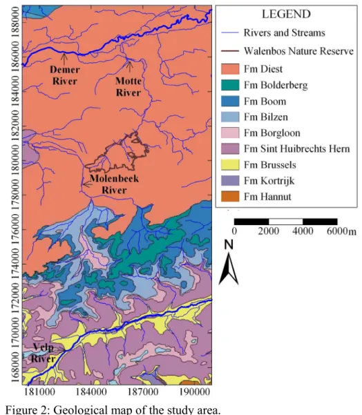
3.2. Geology and hydrogeology 12
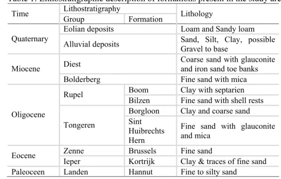
Fig. 2 shows the geological map of the study area. Additionally, Table 1 gives the 13
lithostratigraphic description of the formations present in the study area. The geology of the 14
study area consists of an alteration of sandy and more clayey formations, generally dipping to 15
the north and ranging in age from the Early Eocene to the Miocene. The Hannut formation are 16
clayey or sandy silts with locally a siliceous limestone. The formation only crops out south of 17
the Velp River. The Kortrijk formation is a marine deposit consisting mainly of clayey 18
sediments. This formation is covered by the Brussel formation, a heterogeneous alteration of 19
coarse and fine sands, locally calcareous and/or glauconiferous. The Early Oligocene Sint 20
Huibrechts Hern formation is a glauconiferous or micaeous, clayey fine sand, which is locally 21
very fossiliferous. The Borgloon formation represents a transition to a more continental 22
setting and consists of a layer of clay lenses followed by an alteration of sand and clay layers. 23
The Bilzen formation represents a marine deposit consisting of fine sands, glauconiferous at 24
the base. The Bilzen sands are followed by a clay layer, the Boom formation. On top of the 25
Boom formation, the Bolderberg formation is found which consists of medium fine sands, 26
locally clayey. The youngest deposits consist of coarse, glauconiferous sands of the Diest 27
formation. These sands are deposited in a high energetic, shallow marine setting and have 28
locally eroded underlying formations. In the Walenbos area, for example, the Diest formation 29
is directly in contact with the Brussel formation. The Kortrijk, Brussel and Sint Huibrechts 30
Hern formations are present in the entire study area, while the younger layers disappear 31
towards the south or are eroded in the valleys. The study area is covered with Quaternary 32
sediments, consisting of loamy eolian deposits on the interfluves and alluvial deposits in the 33
river valleys. The geological characteristics of the study area are described in detail in Laga et 1
al. (2001) and Gullentops et al. (2001). 2
3
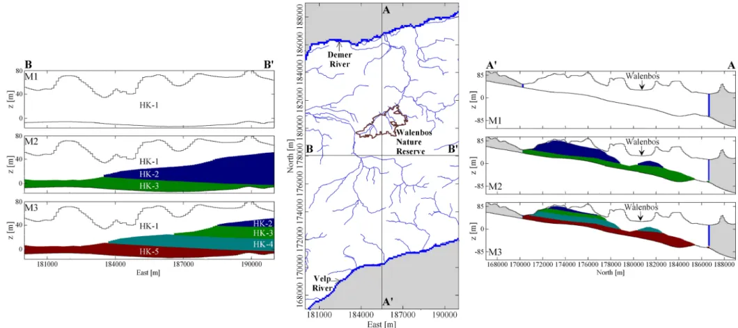
The Hydrogeological Code for Flanders (HCOV) is used to identify different hydrogeological 4
units (Meyus et al., 2000; Cools et al., 2006). The hydrogeological conceptualization of the 5
aquifer system surrounding and underlying the Walenbos Nature Reserve area was 6
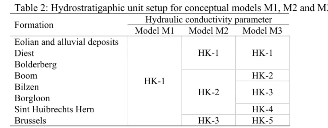
schematized as one-, three- and five-layers with the top of the Kortrijk formation as the 7
bottom boundary for all conceptualizations considered (Fig. 3 and Table 2). These geological 8
models were developed to assess the worth of extra “soft” geological knowledge about the 9
geometry of the groundwater system underlying the Walenbos Nature Reserve. In this way, 10
alternative layering structures for the aquifer are assessed in terms of improving the model 11
performance. 12
13
4. Implementing the multimodel approach 14
Three alternative conceptual models comprising different level of geological knowledge are 15
proposed (Fig. 3). Each model is assigned a prior model probability of 1/3. A complete 16
analysis on the sensitivity of the multimodel methodology to these prior model probabilities is 17
given in Rojas et al. (2009). All proposed conceptual models are bounded by the Kortrijk 18
formation as low permeability bottom and the topographical surface for the top of the system. 19
Model 1 (M1) corresponds to the simplest representation considering one hydrostratigraphic 20
unit, Model 2 (M2) comprises three hydrostratigraphic units and Model 3 (M3) corresponds to 21
the most complex system comprising five hydrostratigraphic units. Details are presented in 22
Table 2 and Fig. 3. 23
24
Groundwater models for the three conceptualizations are constructed using MODFLOW-2005 25
(Harbaugh, 2005). The groundwater flow regime is assumed as steady-state conditions. The 26
model area is ca. 11 × 22 km2. Using a uniform cell size of 100 m the modelled domain is 27
discretized into 110 × 220 cells. The total number of cells varies from model to model since 28
the number of layers to account for different hydrostratigraphic units changed. At the North 29
and South, respectively, the Demer and Velp rivers are defined as boundary conditions using 30
the river package of MODFLOW-2005. Physical properties of both rivers (e.g. width, 31
thickness of bed sediments and river stage) are obtained from models built within the frame of 32
the Flemish Groundwater Model (HAECON and Witteveen en Bos, 2004). All grid cells 33
located to the North of the Demer and to the South of the Velp, respectively, are set as 34
inactive (i.e. no-flow). East and west limits of the modelled domain are defined as no-flow 1
boundary conditions. To account for possible groundwater discharge zones in the study area, 2
the drain package is used for all active cells in the uppermost layer of each model. The 3
elevation of the drain element for each cell is defined as the topographic elevation minus 0.5 4
m, in order to account for an average drainage depth of ditches and small rivulets (Batelaan 5
and De Smedt, 2004). 6
7
The focus of this work is on the assessment of conceptual model and recharge (scenario) 8
uncertainties. Therefore, we confine the dimensionality of the analysis by considering 9
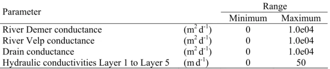
uncertainty only in the conductance parameters related to the Demer and Velp rivers, 10
conductance of drains, and hydraulic conductivities of the alternative hydrostratigraphic units 11
(see Table 2 and Table 3). Additionally, the spatial zonation of the hydraulic conductivity 12
field is kept constant and only the mean values for each hydrostratigraphic unit are sampled 13
using the M-H algorithm. Parameter ranges are defined based on data from previous studies 14
and they are presented in Table 3 (HAECON and Witteveen en Bos, 2004). It is worth 15
noticing that in the frame of the proposed methodology, heterogeneous fields following the 16
theory of Random Space Functions (RSF) are easily implemented (Rojas et al., 2008). 17
18
Average recharge conditions
( )
R over a grid of 100 × 100 m accounting for average 19hydrological conditions is obtained from Batelaan et al. (2007). Spatially distributed recharge 20
values are calculated with WetSpass (Batelaan and De Smedt, 2007), which is a physically 21
based water balance model for calculating the quasi-steady-state spatially variable 22
evapotranspiration, surface runoff, and groundwater recharge at a grid-cell basis. The average 23
recharge condition constitutes the base situation for the estimation of the posterior model 24
probabilities used in the multimodel approach. Additionally, to account for recharge 25
uncertainties (scenarios), two optional recharge situations are defined based on a deviation 26
corresponding to ±2σR from the average recharge conditions
( )
R . We used ±2σRto make 27an intuitive link with the expression of 95% confidence interval for potential recharge values. 28
The definition of these three recharge settings is based on long-term simulations of the 29
average hydrological conditions accounting for more than 100 years of meteorological data 30
(see Batelaan and De Smedt, 2007). Although in a strict sense, the plausibility of these 31
average recharge values might have been evaluated as they took place in the past similarly to 32
the dataset D, this is not possible as D considered a limited and variable time series of head 33
measurements. The key assumptions for the analysis performed in this work are, first, the 1
nature of the steady-state condition of D. This steady-state condition is valid for present-time 2
situation only since the time series available with observed heads are considerably less than 3
the series of meteorological data used to estimate average recharge conditions (S2). Second, it 4
is the fact that there is no guarantee that similar (climate) recharge conditions will be observed 5
for the next 100 years. The latter will have a clear influence on the definition of coherent prior 6
probabilities for each scenario. 7
8
Based on the assumption previously discussed, recharge uncertainties are treated as scenario 9
uncertainties in the context of the proposed GLUE-BMA method (equations 1-4). To avoid 10
conflicting terminology, however, both terms scenario uncertainties and recharge 11
uncertainties are used interchangeably hereafter. 12
13
Based on long-term simulations three recharge conditions (scenarios) are defined: S1 14
(
R 2− σR)
, S2( )
R , and S3(
R 2+ σR)
. Average values for S1, S2 and S3 are 93.1 mm yr-1, 15
205.4 mm yr-1 and 319.5 mm yr-1, respectively. Based on the previous assumption of future 16
recharge conditions, each scenario is assigned a prior scenario probability of 1/3. This is 17
based on the fact that for future recharge conditions, average or tail values are equally likely 18
to be observed. 19
20
A Gaussian likelihood measure is implemented to assess model performance, i.e. to assess the 21
ability of the simulator to reproduce the observed dataset D. Observed heads (hobs) for the 51
22
observation wells depicted in Fig. 1 are compared to simulated heads (hsim) to obtain a
23
likelihood measure. Observed heads correspond to a representative value (average) for steady 24
state-conditions for different time series in the period 1989-2008. Observation wells vary in 25
depth and also the length and depth of the screening is variable. Although some local confined 26
conditions controlled by the Boom formation are observed in the study area, the observed 27
dataset D accounted for phreatic conditions solely. This might lower the information content 28
of the dataset D to effectively discriminate between models. A limited set of head 29
observations, however, may often be the only information available about the system 30
dynamics to perform a modelling exercise and/or model discrimination. From preliminary 31
runs a departure of ± 5 m from the observed head in each observation well is defined as 32
rejection criterion. That is, if hobs−5m<hsim<hobs+5m a Gaussian likelihood measure is 33
calculated, otherwise the likelihood is zero. This rejection criterion is defined in order to 1
achieve enough parameter samples for the exploration of the posterior probability space and 2
to ensure convergence of the different Markov Chains used in the M-H algorithm. For details 3
about the implementation of the rejection criterion in the frame of the proposed approach the 4
reader is referred to Rojas et al. (2008). 5
6
Five parallel Markov Chains, starting from randomly selected points defined in the prior 7
parameter ranges (Table 3), are implemented to proceed with the M-H algorithm for each 8
conceptual model. Four-, six-, and eight-dimensional uniform distributions with initial prior 9
ranges defined in Table 3 are defined as the q
( )
θ* i proposal distributions for M1, M2 and10
M3, respectively. The variance of the proposal distributions is modified by trial-and-error to 11
achieve acceptance rates in the range 20 – 40 %. For each proposed parameter set a new 12
gaussian likelihood value is calculated in function of the agreement between observed and 13
simulated groundwater heads at the 51 observation wells depicted in Fig. 1. These proposed 14
parameter sets are accepted or rejected according to step #6 of section 2.3. As previously 15
stated, the mixing of the chains and the convergence of the posterior probability distributions 16
is monitored using the R-score (Gelman et al., 2004). The resulting total parameter sample 17
(after discarding the burn-in samples) can be considered as a sample from the posterior 18
distribution given the observed dataset D for each alternative conceptual model. This 19
simulation procedure is repeated for models M1, M2 and M3 for average recharge conditions 20
( )
R to obtain the posterior model probabilities (equation 2). 2122
Using the discrete samples from the M-H algorithm the integrated likelihood of each 23
conceptual model, p D
(
Mk)
in equation 2, is approximated by summing over all the retained 24likelihood values for Mk. The posterior model probabilities are then obtained by normalizing 25
over the whole ensemble Μ under average recharge conditions. 26
27
For each series of predicted variables of interest, e.g., river losses and river gains from the 28
Velp and Demer, drain outflows, and groundwater inflows and outflows from the Walenbos 29
area, a cumulative predictive distribution, p
(
Δ D| , M ,Sk i)
, is approximated by normalizing 30the retained likelihood values for each conceptual model under each scenario such that they 31
sum up to one. 32
1
The leading moments of the full BMA predictive distribution accounting for parameter, 2
conceptual model and scenario uncertainties are then obtained using equations (3) and (4). 3
4
5. Results and discussion 5
Since it is not possible to show the complete set of results for all variables, groundwater 6
budget terms and alternative conceptualizations, in the following sections the most relevant 7
results are summarized. 8
9
5.1. Validation of the M-H algorithm results 10
The proposed methodology mainly worked by sampling new parameter sets for each proposed 11
conceptual model following an M-H algorithm with the aim of obtaining posterior parameter 12
probability distributions. Several aspects of the implementation of the M-H algorithm such as 13
the acceptance rate, the definition of the burn-in samples, the proper mixing of alternative 14
chains and the convergence of the first two moments were checked to validate the results 15
obtained using the improved methodology. 16
17
The average acceptance rates for the Markov Chains found for models M1, M2 and M3 (for 18
the 20 000 parameter samples) were 25 %, 23 % and 27 %, respectively. All values lie in the 19
ranges as suggested in literature (Makowski et al., 2002). 20
21
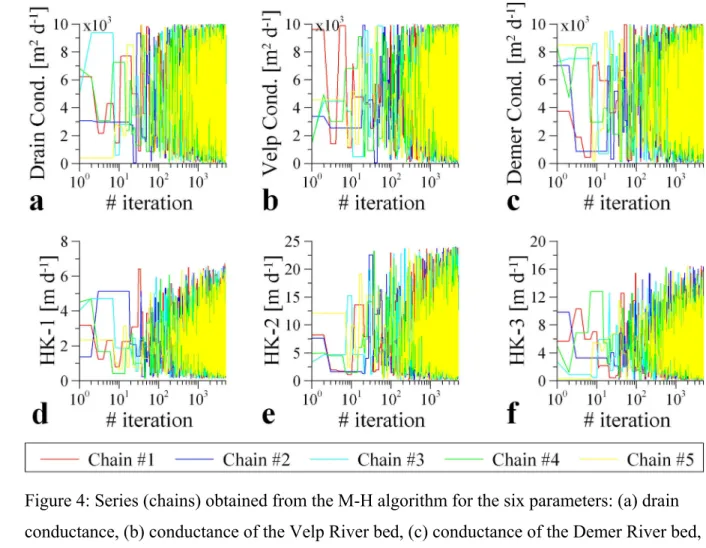
Fig. 4 shows, as an example, five chains for the parameters included in model M2. This figure 22
shows the values for the proposed parameter versus the number of sampling iteration. It is 23
seen that full mixing of the five chains is achieved for values greater than 1 000 parameter 24
samples for all six parameters (plates a through f). As a result, the first 1 000 iterations were 25
set as burn-in samples and they were discarded as they were slightly influenced by the starting 26
values of the chains. Although not shown here, similar results were obtained for models M1 27
and M3, with 1 000 initial samples defined as burn-in. 28
29
As previously stated, the mixing of the chains and the convergence of the posterior probability 30
distributions of parameters and variables of interest were monitored using the R-score. 31
Gelman et al. (2004) suggest values for the R-score near 1, with values below 1.1 acceptable 32
for different problems. The R-score was calculated for the whole series of parameters and 33
variables of interest for the three alternative conceptual models M1, M2, and M3. The largest 34
R-score for 5 000 parameter samples was 1.02 indicating a good mixing of the five chains 1
and, hence, suggesting convergence of the posterior probability distributions (e.g. see how all 2
five chains completely overlap in Fig. 4 after a value of 1 000 for the case of M2, covering the 3
same support for the posterior probability distributions). Subsequently, a discrete parameter 4
sample comprising 20 000 values is obtained by combining the results of the five chains. 5
6
Although not shown here, convergence of the first two moments for the posterior distributions 7
of parameters obtained from the total discrete parameter sample was also confirmed for the 8
three alternative conceptual models. 9
10
Therefore, the resulting discrete samples of parameters from models M1, M2 and M3 can be 11
considered as a sample from the target posterior distributions under the respective conceptual 12
model. 13
14
5.2. Likelihood response surfaces 15
From the proposed methodology, each parameter set was linked to a likelihood value. The 16
resulting marginal scatter plots of parameter likelihoods for models M1 and M2 are shown in 17
Fig. 5 and Fig. 6, respectively. Also, included in these figures are the results of a weighted 18
least squares calibration using UCODE-2005 (Poeter et al., 2005). It is worth mentioning that 19
several calibration trials (six for Model M1, ten for model M2 and more than twenty for 20
model M3) starting at different initial parameter values contained in the ranges defined in 21
Table 3 were launched. For the sensitive parameters all the calibration trials converged to 22
rather similar optimum parameter values, however, some minor differences were observed 23
due to irregularities in the likelihood response surface. For insensitive parameters, on the 24
other hand, different trials converged to different values. For the sake of clarity, only the final 25
calibrated parameter set is included in the comparison with the GLUE-BMA results. 26
27
From Fig. 5 and Fig. 6 it is seen that likelihood values were rather insensitive to the 28
conductance of drains and rivers (plates a, b c in Fig. 5 and Fig. 6). High likelihood values 29
were observed for almost the whole prior parameter sampling range being very difficult to 30
identify a well-defined attraction zone for these three parameters. This insensitivity was also 31
reflected in the significant difference between the values obtained using least squares 32
calibration and the highest likelihood points obtained in the context of the proposed method. 33
Clearly, least squares calibration did not succeed in identifying the point and/or even the 34
range where the highest likelihood values for these parameters were observed. This is a well-1
known drawback of least squares calibration methods in the presence of highly insensitive 2
parameters. 3
4
For parameters defining the mean hydraulic conductivity for each model layer, on the 5
contrary, well-defined attraction zones were identified by the proposed methodology (plates d 6
in Fig. 5 and plates d, e and f in Fig. 6). For these parameters, results obtained from least 7
squares calibration were almost identical to the highest likelihood points identified in the 8
frame of the proposed methodology. 9
10
Although not shown here, the same patterns were observed for model M3 for the case of the 11
three insensitive parameters and the parameters defining the mean hydraulic conductivity for 12
layer 1 (HK-1), layer 4 (HK-4) and layer 5 (HK-5) (Table 2). For these last three parameters, 13
well-defined attraction zones were identified and results of least squares calibration were 14
fairly similar to the highest likelihood points identified in the frame of the proposed 15
methodology. However, two exceptions are worth mentioning. In Fig. 7 the marginal scatter 16
plots of calculated likelihood for the hydraulic conductivity of layer 2 (HK-2) (plate a) and 17
layer 3 (HK-3) (plate b) for model M3, are shown. These layers correspond to the Boom 18
formation and Ruisbroek formation, respectively (Table 2). These marginal scatter plots show 19
that likelihood values are fairly insensitive to these two parameters (HK-2 and HK-3) for M3. 20
However, a clear attraction zone for values greater than 0.001 m d-1 is observed for both 21
parameters. This contrasts with the results obtained using the least squares calibration method. 22
The most severe difference is for the case of the parameter HK-2 (plate a) where the highest 23
likelihood point identified with the proposed methodology and the result from the least 24
squares calibration differed by more than six orders of magnitude. It is worth mentioning that 25
convergence of UCODE-2005 was highly sensitive to the initial values of HK-2 and HK-3. 26
After a significant number of trials, meaningful initial parameter values for HK-2 and HK-3 27
were set to 0.01 m d-1 and 4.6 m d-1, respectively. These initial values allowed for 28
convergence of UCODE-2005, however, they produce rather dissimilar calibrated values 29
compared to the highest likelihood points obtained with the proposed methodology. On the 30
contrary, for the case of the proposed methodology the parameters were sampled from the 31
prior range defined in Table 3 following the acceptance/rejection rule described in step # 6 of 32
section 2.3. Therefore, this procedure allowed identifying clear zones of attraction for these 33
two parameters although their insensitivity remained observed. 34
1
This critical difference in both approaches (GLUE-BMA and WLS calibration) may be 2
explained by the meaning and the type of information conveyed by the dataset D in this 3
application. For pragmatic reasons, the dataset D did not include observation wells located in 4
local confined aquifers distributed over the study area since the interest was on the general 5
functioning of the aquifer system and not on local conditions. In general, these local confined 6
aquifers are controlled by the presence of the hydrostratigraphic unit defined by the Boom 7
Formation and, thus, by parameter HK-2. Therefore, if the dataset D, which corresponds to 8
head measurements accounting for phreatic conditions solely, does not contain any relevant 9
information on confined areas it is difficult to account for the relevance and the actual value 10
of parameter HK-2. As a consequence, parameter HK-2 becomes redundant and the zone of 11
attraction defined in Fig. 7a is defined for an “equivalent” parameter accounting only for a 12
phreatic system. This situation was easily assimilated by the GLUE-BMA methodology 13
whereas the WLS method faced convergence problems since initial values for parameter HK-14
2 were defined in the observed range for the hydraulic conductivity values of the Boom 15
Formation. 16
17
Despite these differences between WLS and GLUE-BMA, both methods performed equally 18
well in terms of model performance. As an example, the root mean squared error (RMSE) for 19
model M1 using WLS and GLUE-BMA was 1.884 and 1.876, respectively. For model M2 20
both WLS and GLUE-BMA gave an RMSE of 1.890 whereas for model M3 the RMSE of 21
WLS and GLUE-BMA was 1.761 and 1.741, respectively. 22
23
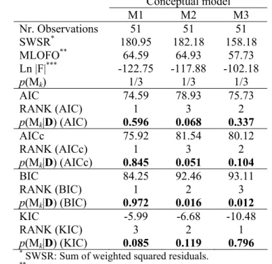
5.3. Posterior model probabilities 24
Table 4 presents the posterior model probabilities obtained using equation (2) for average 25
recharge conditions as a result of the proposed methodology. It is seen from this table that the 26
integrated likelihoods for models M1, M2 and M3 differ slightly. As a consequence, and since 27
posterior model probabilities are proportional to the integrated likelihoods when prior model 28
probabilities are set equal (i.e. when there is no clear preference for a given conceptual 29
model), posterior model probabilities also differ marginally. 30
31
For this case, information provided by the observed dataset D (in the process of updating the 32
prior model probabilities) is marginal and does not allow discriminating significantly between 33
models once D has been observed. This suggests that, for the problem at hand and for the 34
level of information content of D, prior model probabilities will likely play a significant role 1
in determining the posterior model probabilities. In this regard, prior model probabilities 2
could be thought of as “prior knowledge” about the alternative conceptual models. This prior 3
knowledge is ideally based on expert judgement, which Bredehoeft (2005) considers the basis 4
for conceptual model development. In this way, expert “subjective” prior knowledge about 5
optional conceptualizations in combination with the information provided by the dataset D, 6
may allow some degree of discrimination between models through updated posterior model 7
probabilities. As shown in Ye et al. (2008b), however, even for the case when an expert 8
assigns substantially different prior model probabilities, aggregating the prior model 9
probabilities values from several authors gives a relatively uniform prior model probability 10
distribution. It would be interesting to investigate the joint effect of data and expert judgement 11
on the prior model probabilities. For a complete analysis on the sensitivity of the results of the 12
proposed methodology to different prior model probabilities, which is beyond the scope of 13
this article, the reader is referred to Rojas et al. (2009). 14
15
Another possible strategy is to increase the information content of D by collecting new data 16
that may be particularly useful in discriminating between models (e.g. river discharges, tracer 17
travel times and observed groundwater flows). With extra data, the level of “conditioning” of 18
the results is increased and (hopefully) the integrated model likelihoods will differ for 19
alternative conceptual models. In practice, however, a set of observed groundwater heads may 20
often be the only information available about the system dynamics to estimate posterior 21
model probabilities for a set of alternative model conceptualizations. This clearly put the 22
challenge of assigning model weights (i.e. posterior model probabilities) considering often a 23
minimum level of information. 24
25
5.4. Groundwater model predictions accounting for conceptual model and scenario 26
uncertainties 27
Using the posterior model probabilities obtained for average recharge conditions (Table 4) 28
and the cumulative predictive distributions obtained for each model, a multimodel cumulative 29
predictive distribution is obtained for scenarios S1, S2 and S3. 30
31
Fig. 8 shows the cumulative predictive distributions for a series of groundwater budget terms 32
and the combined BMA prediction accounting only for conceptual model uncertainty for 33
scenario S2. From this figure it is seen that, although posterior model probabilities differ 34
slightly (Table 4), indicating a low information content of the dataset D, there are significant 1
differences in the predictions of models M1, M2 and M3. For river losses and river gains from 2
the Demer (plates a and b) and Walenbos outflows and inflows (plates f and g), both the most 3
likely predicted values (P50) and the 95 % (P2.5 - P97.5) prediction intervals drastically differ 4
between alternative conceptual models. This indicates that conceptual model uncertainty 5
considerably dominates both the most likely predictions and the predictive uncertainty under 6
S2. On the other hand, the most likely predicted values for river losses and river gains from 7
the Velp (Fig. 8 plates c and d) and drain outflows (plate e) are rather similar, yet the 95 % 8
prediction intervals span clearly different ranges. This indicates that although the most likely 9
predicted values for models M1, M2 and M3 are quite similar, their predictive uncertainty is 10
largely dominated by conceptual model uncertainty. 11
12
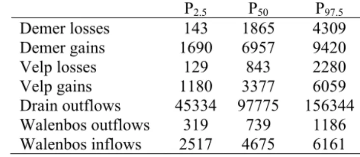
Additionally, Table 5 summarizes the most likely predicted values and the 95 % predictive 13
intervals for models M1, M2 and M3, under scenarios S1, S2 and S3 for the same 14
groundwater budget terms described in Fig. 8. This table shows that for scenarios S1 and S3, 15
uncertainties due to the specification of alternative conceptual models also play an important 16
role. Conceptual model uncertainty is more relevant (under S1) for river gains and river losses 17
from the Demer and the Velp and, marginally, for drain outflows. This is explained by the fact 18
that during low recharge conditions (S1) rivers contribute more water to the groundwater 19
system due to lower simulated groundwater heads in the neighbouring areas. This lowering in 20
heads also explains why the drain outflows are only marginally affected by the conceptual 21
model uncertainty. For scenario S3 all predictive intervals for the groundwater budget terms 22
are affected by the selection of an alternative conceptual model. This is expected as for high 23
recharge conditions (S3) it is likely that all groundwater flow components will be affected by 24
an alternative conceptualization. 25
26
A slight tendency to larger predictive intervals for M3, then M2 and, finally, M1 is observed 27
for all recharge conditions. This is expected as an increase in model complexity, expressed as 28
an increase in the number of model parameters, allows for more parametric uncertainty to be 29
incorporated. This suggests that model M3 will produce the main contribution to conceptual 30
model uncertainty due to wider predictive intervals. 31
32
If groundwater budget terms are transversely analyzed it is seen that predictive intervals for 33
river losses are dominated by scenario S1 whereas predictive intervals for rivers gains are 34