ATMOSPHERIC PERTURBATIONS ON GNSS SIGNALS AND THEIR INFLUENCE ON
TIME TRANSFER.
René Warnant
Royal Observatory of Belgium 3, Avenue Circulaire B-1180 Brussels (Belgium) Email : [email protected] ABSTRACT
The paper reviews the influence of atmospheric perturbations acting on precise time tranfer applications based on Global Navigation Satellite Systems (GNSS). The Earth atmosphere (ionosphere and troposphere) induces a propagation delay on the signals emitted by GNSS. The tropospheric error can be modelled satisfactorily but the ionosphere remains an important error source. The paper reviews the main disturbances due to the ionosphere and, in particular, shows the influence of solar activity on these disturbances.
INTRODUCTION
Time transfer using GNSS signals is affected by the atmospheric refraction. This effect has two components: the tropospheric error which is the effect of the neutral atmosphere and the ionospheric error which is the effect of the ionized atmosphere. The tropospheric error is usually removed using a classical tropospheric model like the Hopfield model or the Saastamoinen model which can lead to residual errors up to 0.2 ns (at zenith) due to the high variability of water vapour in the atmosphere. In practice, the residual error is negligible for time transfer applications using code measurements. For this reason, we focus our attention on the ionospheric error. One way to take this effect into account consists in forming the so-called geometric free combination of the code measurements made on the 2 frequencies emitted by the GNSS when dual frequency receivers are available. This combination has the advantage to remove the ionospheric effect but has the inconvenient to increase the measurement noise in a way which is significative with respect to the accuracy of time transfer. When only single frequency measurements are available, the ionospheric effect is usually taken into account by correcting GNSS observations with the Klobuchar model. In addition, clock comparisons are made by forming differences between observations collected in neighbouring stations; one usually assumes that the residual ionospheric error remaining in the differences is negligible. The aim of the paper is to demonstrate that this assumption is not valid under disturbed ionospheric conditions which are often observed during periods of high solar activity. The analysis is based on a study of the ionospheric Total Electron Content (TEC) performed at the Royal Observatory of Belgium using 9 years of observations, nearly one solar activity cycle.
THE IONOSPHERIC REFRACTION
GPS satellites emit two carrier frequencies, L1 (1575.42 Mhz) and L2 (1227.6 Mhz) modulated by two codes called C/A code and P code. Both types of signals are refracted when crossing the ionosphere: the codes undergo a path lengthening, I and the carriers, a path shortening, -I. Neglecting higher order terms in the signal frequency, f, the ionospheric error, I, expressed in metres is given by:
The Total Electron Content (TEC) is the integral of the electron density on the receiver-to-satellite path. The TEC is measured in electrons m-2 or in TEC units (TECU) where 1 TECU = 1016 électrons m-2. The relation between slant and
vertical Total Electron Content, TEC and , is usually given by:
-180 -135 -90 -45 0 45 90 135 180 Longitude -90 -45 0 45 90 Lati tude
Figure 1. The regions of the ionosphere.
The Total Electron Content is very variable both in space and time. It is a function of geomagnetic latitude, local time, season, solar cycle, ... For this reason the TEC is very difficult to model. The ionosphere is usually divided in 3 regions depending on geomagnetic latitude (figure 1):
- the polar region where the TEC is the most variable and irregular; in this region, the TEC behaviour is strongly dependent on geomagnetic activity;
- the mid-latitude region where the TEC and its gradient are the lowest and the most regular; - the equatorial region where the highest TEC gradients and TEC values are observed.
In Table 1, the ionospheric error on a one way C/A code measurement is given (in ns) for 3 values of the TEC: - 20 TECU: a very usual value encountered at all latitudes independently of solar activity;
- 100 TECU: a usual value for the equatorial region and a “maximum” value for mid-latitude stations during periods of high solar activity;
- 200 TECU: a very high value encountered only in the equatorial region during periods of very high solar activity. Table 1. Ionospheric delay (ns) on C/A code.
TEC Delay C/A code
Z = 0/ Z = 70 /
200 108 316
100 54 158
20 11 32
METHODS USED TO CORRECT THE IONOSPHERIC ERROR Klobuchar model
A first way to correct GPS measurements for the ionospheric refraction effect is to use a prediction model of the TEC. Such models are usually able to predict the TEC in function of several parameters as local time, latitude, solar activity, ... They are based on monthly average TEC profiles. An example is given by the Klobuchar model [2] of which the 8 parameters are broadcast in the GPS satellite navigation message. Unfortunately, the TEC often discards form its monthly average behaviour. This fact is illustrated further in the paper. In practice, this model can only be considered as a first approximation giving rise to important residual errors under disturbed ionospheric conditions.
0:00 4:00 8:00 12:00 16:00 20:00 0:00 0 5 10 15 20 25 30 T E C ( T ECU) November 1994 0 4 8 12 16 20 24 Local Time 0 50 100 T E C ( T EC U) November 2001 0:00 4:00 8:00 12:00 16:00 20:00 0:00 0 5 10 15 20 25 30 T E C ( T ECU) December 1994
The “common view” method
The so-called “common view” time transfer technique uses differences of one way code observations made in 2 different stations on the same satellite which is in view at both sites. One advantage of the method is to remove all the errors common to both measurements. In particular, if the station interdistance is small, one can expect that the ionosphere (i.e. the TEC) above these stations is very similar and in consequence, the ionospheric refraction effect on the two measurements made in these two neighbouring stations will be the same. In this case, the “common view” measurement is (nearly) not affected by the ionospheric refraction. When the distance between the stations increases, the ionospheric residual error increases accordingly. In practice, the residual ionospheric error remaining in the common view observations depends on: - the gradients in the vertical TEC between the two observing stations;
- the vertical TEC itself; indeed, even if the vertical TEC has the same value at both sites, there remains a residual error: this is due to the fact that the two receivers are observing the satellite with a different zenith angle.
As a consequence, the Total Electron Content and its gradients in space have to be studied in order to evaluate the residual ionospheric error remaining in the single differences.
STUDY OF THE VERTICAL TEC
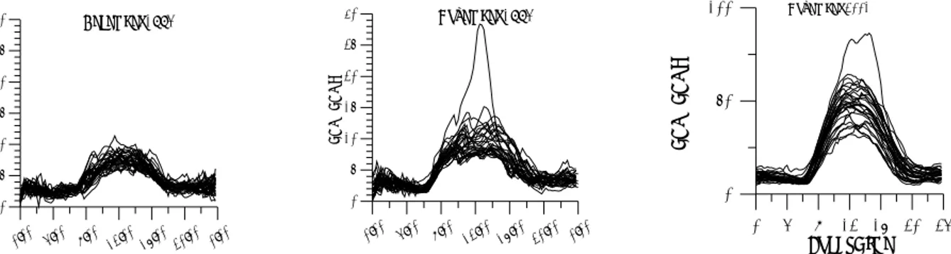
GPS code and carrier phase measurements can be combined in order to compute TEC profiles in function of local time with a precision of 2-3 TECU. A description of the method used by the author can be found in [1] and [4]. This method has been applied to GPS measurements collected at Brussels (50.8
/
N) on a period of 9 years (April 1993-March 2002). Figure 2 shows all the daily TEC profiles obtained at Brussels in November 1994, December 1994 and November 2001: all the TEC profiles corresponding to the same month are represented on the same graph.Figure 2. Daily TEC profiles at Brussels in function of local time in November 1994, December 1994 and November 2001. From this figure, it can be seen that the TEC curves have a rather evident day-to-day repeatability (see December 94, in particular). Nevertheless, in many cases, the TEC discards from its monthly average value : see for example, November 94 (low solar activity) and November 2001 (high solar activity), where the difference between the monthly average value and the real value reaches about 50 TECU. This difference would lead to an error of 27 ns at zenith on a one way C/A code measurement. It is also important to underline that Brussels is located in the mid-latitude region (i.e. the quietest region of the ionosphere). In other words, the use of the Klobuchar ionospheric model to correct single frequency data for the ionospheric effect can lead to large residual errors. Figure 3 (left) shows the dependence of the mean daily TEC on solar activity.
STUDY OF THE TEC GRADIENTS
The gradients in the TEC can be divided in 2 classes:
- the regular gradients: the “usual” gradients observed in the TEC; for example, the TEC has a minimum value during the night and reaches its maximum around 14h00 (local time). Consequently, there is a gradient depending on local time; another example: in the equatorial region during high solar activity, North-South gradients of about 30 TECU per 100 km are observed [3] and gradients of 100 TECU between the equatorial and the mid-latitude regions are not unusual during periods of high solar activity. For this reason, common view experiments between 2 equatorial stations or between a mid-latitude station and an equatorial station could lead to large residual ionospheric errors.
Time ( Years ) 0 400 800 1200 1600 N u m ber of det ec ted ev ent s p e r m ont h 1993 1994 1995 1996 1997 1998 1999 2000 2001 2002 2003 1992 1994 1996 1998 2000 2002 2004 Time ( Years ) 0 10 20 30 40 50 Me a n d a ily T E C (T E C U )
scintillation effects. Travelling Ionospheric Disturbances or TID’s appear as waves in the electron density (and consequently
in the TEC) due to interactions between the neutral atmosphere and the ionosphere. They have a wavelength ranging from a few tens of kilometers to more than thousand kilometers. Their occurrence often cause important gradients in the TEC even on a few kilometers. Scintillation effects are variations in phase and amplitude of a radio signal passing through small scale irregularities in the ionosphere. Scintillation effects are very often observed in the polar and equatorial regions and are sometimes detected in the mid-latitude region, in particular, during geomagnetic storms. These phenomena also give rise to important and very irregular changes in the measured TEC. The GPS data bank archived at the Royal Observatory of Belgium has been used in order to detect the occurrence of TID’s and scintillations at Brussels. Figure 3 (right) shows the number of ionospheric irregular phenomena (TID’s or scintillations) observed per month from April 93 to March 2002. Most of the events represented on this figure are due to TID’s which are very often observed in mid-latitude regions even if solar activity is low. Scintillation effects were also observed during geomagnetic storms on the period 2000-2002. On the period covered by our data set, we have observed that the occurrence of TID’s and scintillations at Brussels leads to difference of 2 to 6 TECU between the TEC measured in stations separated by about 50 km (1.1 to 3.3 ns at zenith on C/A code). In the case of an equatorial station, differences of 12 TECU (6.5 ns at zenith) due to scintillation effects have been reported in the literature for similar station interdistances. It is important to underline that the total ionospheric effect is the sum of the regular and irregular gradients. Indeed, in some cases, even if the effect of the irregular part can be considered as non significative, the total effect (regular + irregular) could become significative.
Figure 3. Left: Mean daily TEC from April 1993 to March 2002; Right: Number of irregular ionospheric phenomena observed per month from April 1993 to March 2002.
CONCLUSIONS
The ionospheric effect remains a non-negligible error source in time transfer using C/A code measurements. This effect increases tremendously during periods of high solar activity. The use of the Klobuchar model, which is based on a monthly mean TEC behaviour to correct the measurements for the ionosphere can lead important errors particularly when clock comparisons are made between a mid-latitude and an equatorial station and when scintillations effects are present. REFERENCES
[1] G. E. Lanyi et T. Roth (1988): A comparison of mapped and measured total ionospheric electron content using global positioning system and beacon satellite observations, Radio Science, 23, 483-492.
[2] J.A. Klobuchar (1986): Design and characteristics of the GPS ionospheric time delay algorithm for single frequency users, Proceedings of the PLANS-86 conference, Las Vegas, Nevada, 280-286.
[3] Wanninger L. (1993), Effects of equatorial ionosphere on GPS, GPS World, July, 48.
[4] Warnant R. and E. Pottiaux (2000), The increase of the ionospheric activity as measured by GPS, Earth, Planets and Space, Vol.52, 11, pp. 1055-1060.