HAL Id: hal-01796103
https://hal.archives-ouvertes.fr/hal-01796103
Submitted on 28 May 2018
HAL is a multi-disciplinary open access
archive for the deposit and dissemination of
sci-entific research documents, whether they are
pub-lished or not. The documents may come from
teaching and research institutions in France or
abroad, or from public or private research centers.
L’archive ouverte pluridisciplinaire HAL, est
destinée au dépôt et à la diffusion de documents
scientifiques de niveau recherche, publiés ou non,
émanant des établissements d’enseignement et de
recherche français ou étrangers, des laboratoires
publics ou privés.
Freeform optics complexity estimation: comparison of
methods
Eduard Muslimov, Emmanuel Hugot, Simona Lombardo, Melanie Roulet,
Marc Ferrari
To cite this version:
Eduard Muslimov, Emmanuel Hugot, Simona Lombardo, Melanie Roulet, Marc Ferrari. Freeform
optics complexity estimation: comparison of methods. SPIE PHOTONICS EUROPE, Apr 2018,
Strasbourg, France. �hal-01796103�
Freeform optics complexity estimation: comparison of methods
Eduard Muslimov
*a,b, Emmanuel Hugot
a, Simona Lombardo
a, Melanie Roulet
a, Marc Ferrari
aa
Aix Marseille Univ, CNRS, CNES, LAM, Laboratoire d'Astrophysique de Marseille, 38, rue
Joliot-Curie, Marseille,13388, France;
bKazan National Research Technical University named after A.N.
Tupolev –KAI, 10 K. Marx, Kazan 420111, Russia
ABSTRACT
In the present paper we compare different approaches for estimation of freeform and aspherical surfaces complexity. We consider two unobscured all-reflective telescope designs: a narrow-field Korsch-type system with a slow freeform secaondary and a wide-field Schwarzschild-type system with an extreme freeform secondary. The performance improvement obtained due to the freeforms use is demonstrated. The Korsch telescope provides a diffraction-limited image quality for a small field 0.8x0.1º at F/3. The Schwarzschild design covers a large field of 20x8º and allows to increase the aperture from F/6.7 to F/3. Also, we analyze the freeforms shapes using different techniques. It is shown that the usual measures like root-mean square deviation of the sag are ineffective. One of the recommended way to estimate the surface complexity is computation of the residual slope and its conversion into fringes frequency. A simpler alternative is computation of the sag deviation integral.
Keywords: freeform optics, optical design, manufacturability, interferometric testing, asphericity gradient
1. INTRODUCTION
Imaging freeform optics is a rapidly emerging field, which allows to build optical systems with previously unachievable performance. Use of the freeform surfaces allows to achieve a better aberrations correction, and therefore to increase the resolution and/or create optical systems with a smaller f-number, wider field of view and smaller dimensions. However, use of the freeform optics requires a certain revision of the optical design process. Particularly, it is necessary to estimate and control the freeform surface complexity during the design and optimization in order to obtain a manufacturable and cost-effective solution. The complexity criteria, which were previously introduced for rotationally-symmetric aspheres based on the conic sections cannot be directly applied to freeforms1,2.
The common way to demonstrate the freeform complexity is deviation from the best-fit sphere. This method is simple, but it can lead to misevaluation of manufacturability, because many of the freeforms manufacturers do not use spherical blanks, but grind directly to the freeform shape3. In addition, there are different ways to quantify this deviation from the
basic geometry. The results may vary depending on the assumptions about the clear aperture shape and size, as well as on usage of the root-mean square (RMS), peak-to-valley (PTV) or integral values.
Another approach to estimation of the surface complexity is derived from the capability to measure the exact shape of the surface. The most of the manufacturers emphasize that measurement is the key point in the aspheres and freeforms fabrication chain. In this case the complexity is assessed by the surface slope steepness4-6. This approach is related to the
fact that the majority of optical testing techniques rely on interferometry, and therefore the slope is often represented as the fringes frequency. In contrast with the first approach this is directly related to the testing process but requires additional computations.
Thus the main goal of the present study is to compare different methods of the surface complexity estimation in the application to freeform surfaces and demonstrate a correlation between them, the advantages and shortcomings for each of them.
In order to cover different cases, we consider two different optical designs. The first one is a Korsch-type unobscured telescope scheme with three mirrors7. As we show below, the design re-optimization with a freeform secondary leads to
a solution with a slow freeform mirror, which has a rectangular aperture. The second example design is a two-mirror
unobscured telescope based on Schwarzschild geometry8. In turn, this design uses a freeform with large deviations and a
nearly circular aperture. A more detailed description of the designs is given in Section 2; Section 3 demonstrates the gain in the image quality achieved with the freeforms and the Section 4 provides the surface shape analysis. The general conclusions on the study are given in Section 5.
2. SAMPLE OPTICAL DESIGNS
For the demonstrative purposes we consider the two unobscured reflective telescope designs. In both of the cases we use a known design based on off-axis aspheres as the starting point. The main optical parameters for the initial and resultant designs are summarized in Table 1.
Table 1. The main parameters of the demonstrative optical designs.
Korsch telescope Schwarzschild telescope Initial Re-designed Initial Re-designed Surfaces
configuration
3 off-axis conic-based aspheres
2 off-axis conic-based aspheres and a freeform
secondary
2 off- axis aspheres: 2nd
order primary and 8th
order secondary
Centered aspherical primary and centered
freeform secondary
Focal length, mm 500 500 500 500
F-number 4 4 6.7 3
Field of view, º 0.8x0.1 0.8x0.1 20x8 20x8
2.1 Korsch telescope
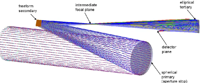
The Korsch-type design has a moderate f-number and a small field of view (FoV). The field is rectangular and has the aspect ratio of 8. Such a telescope could be used to feed a spectrograph. The general view of the optical design is presented on Fig.1. The freeform surface is introduced on the second mirror, while the aperture stop is on the primary mirror. The freeforms described by the standard Zernike sag polynomials9. 7 modes, namely the defocus, the 3rd order
astigmatism coma and trefoil, the primary spherical and the 5th order astigmatism are used. The entire system is
re-optimized, but its principal geometry is maintained.
2.2 Schwarzschild telescope
The second sample design is also an unobscured telescope. It has a wide field of view and intended for imaging. The initial design is an off-axis part of the Schwarzschild scheme with two aspheric mirrors having approximately equal vertex radii. The first mirror is a conicoid and the second one is an even asphere with 3 additional coefficients. The aperture stop is on the secondary mirror. In contrast with the previous case the design was subject to a considerable revision. Firstly, each of the off-axis aspheres were turned into a surface, which has the vertex coinciding with the aperture center. Secondly, the a freeform was introduced on the secondary mirror. The shape is described by the standard Zernike sag polynomials as well. 11 modes, including all the YZ-symmetric terms from Z3 to Z22 are used. Finally, since
the application of freeform allows to increase the image quality dramatically it was decided to change the f-number from 6.7 to 3. The entire optical system was also re-optimized with these new conditions and maintenance of the principal geometry. The general view of obtained design is shown on Fig.2.
Figure 2. General view of the Schwarzschild-type telescope design (f’=500 mm, F/3, 20ºx8º).
3. IMAGE QUALITY ANALYSIS
Below we investigate the image quality parameters of all the optical design configurations mentioned before. It is evident that use of the freeform surfaces allows to achieve a substantial gain in the image quality.
3.1 Korsch telescope
The spot diagrams for the Korsch-type telescope designs are given on Fig. 3. For the initial configuration the spot radius RMS at 550 nm varies between 2.7 and 3.7 µm. For the optical system with a freeform the corresponding values are 0.85-0.92µm. One also can clearly see that in the second case the spot size is smaller than the Airy disk diameter, which is equal to 5.2 µm, i.e. the telescope becomes a diffraction-limited system. For these reason we do not provide other estimations of the image quality for this telescope.
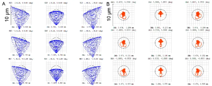
Figure 3. Spot diagrams of the Korsch-type telescopes (the black circles show the Airy disk diameter; the reference wavelength is 550 nm): A – initial configuration with off-axis aspheres; B –the resultant freeform-based design-optimized.
3.2 Schwarzschild telescope
In a similar way we provide the spot diagrams for the second, Schwarzschild-type, telescope (see Fig.4). The spot RMS radii for the initial configuration are 13.0-35.2 µm, while for the design with a freeform they are 10.3-13.6µm. So the gain in the spot size for the FoV corner is as big as factor of 2.6. One also should keep in mind the decrease of the F-number from 6.7 to 3.
Figure 4. Spot diagrams of the Schwarzschild-type telescopes (the reference wavelength is 550 nm): A – the initial configuration with off-axis aspheres at F/6.7; B – the resultant freeform-based design at F/3.
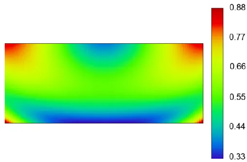
This telescope design provides relatively high image quality over the extended FoV. In order to visualize this quality and to facilitate comparison with other similar designs10 we provide the field map (see Fig.5). One can note that the
Figure 5. RMS wavefront field map for the Schwarzschild-type design (the units on colorbar are waves).
4. FREEFORM SURFACES ANALYSIS
The freeform complexity analysis was performed in a similar way for all the designs and configurations. The actual surface was fitted with a spherical or toroidal surface. The latter shape can be useful if the freeform shape is dominated by the astigmatic term. It was supposed that the radii of curvature and all the coordinates of the center of fitting surface were free variables. The RMS deviation between the actual surface and the fitting one was minimized using a standard simplex-method11 over the actual clear aperture. Then the residual deviation is estimated in different ways. The RMS
and PTV sag deviations are calculated. Also the integral of the deviation, i.e. the volume of the deviation is computed. Finally, the slope of the deviation is calculated and converted into frequency of interference fringes. We assume that the reference wavefront matches the best fit surface so the fringes frequency is related to the residuals instead of the entire sag. The reference wavelength for the fringes frequency computation is 532 nm in all the cases.
4.1 Slow freeform in the Korsch design
Since the freeform mirror is out of the aperture stop position and the FoV is rectangular, the actual clear aperture of the surface is rectangular as well. The best fit sphere (BFS) has the radius of -383.063 mm and decentered by (0, 0.161, 0.004) in mm. The residual sag deviation is shown on Fig.6A. One can note that the deviation is relatively small with the PTV value of only 11.6 µm. Fig.6B demonstrates the vectorial field of the deviation gradient. The same computations were made for the case of fitting with a toroid.
For comparison we provide the results of analysis for the initial off-axis asphere, which was performed in the same way. All the data are summarized in table 2. Considering these data one can note a few points. Firstly, all the estimates show that the mirrors are relatively easy in fabrication. Secondly, comparing with a best fit tor is inapplicable for an ordinary asphere, but it can be useful for some aspheres. The third point is related to the relative change of the estimate. For instance, the RMS sag deviation from the BFS is the same for the ordinary asphere and the freeform. At the same time, the change of the integral deviation is 26% and that of the fringes frequency is 11%. In addition, the integral deviation is proportional to the amount of removed material and the fringes frequency is the parameter defining the interferometric testing possibility, while the RMS deviation does not directly correspond to any technological limitation.
So, for slow aspheres and freeforms computation of the RMS sag deviation is not a preferable way to estimate the surface complexity, because of its low sensitivity to the shape changes and absence of a direct connection with the fabrication or testing limitations.
Figure 6. Residuals analysis for the freeform secondary in the Korsch-type design: A – residual sag (the units are microns), B – slope of the residuals.
Table 2. Analysis of the Korsch telescope secondary mirror asphericity. Initial design,
off-axis asphere
Resultant design, freeform
Fitting surface Sphere Toroid Sphere Toroid RMS deviation, µm 0.4 0.9 0.4 0.5 PTV deviation, µm 10.1 21.2 11.6 11.1 Integral deviation, mm3 1.04 2.28 1.31 0.94 Slope 0.0010 0.0016 0.0012 0.0011 Fringes frequency at 532 nm, mm-1 3.94 5.96 4.38 4.24
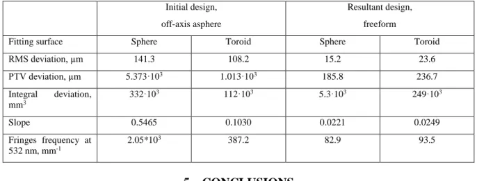
4.2 Steep freeform in the Schwarzschild design
In contrast with the previous case, the freeform surface position coincides with the pupil, so the clear aperture is circular. So the computation was performed over this circular shape and with a radial grid. The rest of the procedure was similar to the one used for the previous design.
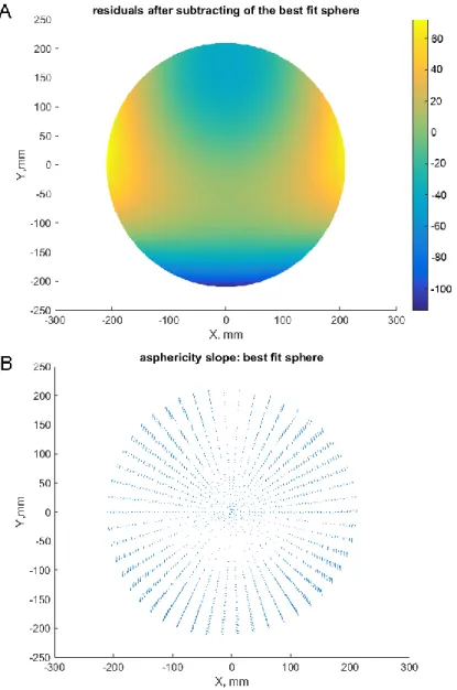
The BFS has radius of -1410.1 mm and its center coordinates are (0, 0.0004, 0) mm. The residual sag deviation is shown on Fig.7 A. The PTV value reaches 185.8 µm. Typically, such a freeform is considered as a complex one. The deviation gradient map is shown on Fig.7B. The rest of the complexity estimates are given in Table 3. It should be noted that for the BFS computations with the decentered ordinary asphere an additional tilt term was introduced.
One can see from the table that due to the decenter, which is large big as 634.5mm, the ordinary asphere has a huge asphericity. So regardless of the complexity estimation approach the aspherical secondary mirror in the starting point design appears to be extremely complex for fabrication. However, the results strongly depend on the reference surface.
Figure 7. Residuals analysis for the freeform secondary in the Schwarzschild-type design: A – residual sag (the units are microns), B – slope of the residuals.
In contrast, the freeform can be considered as manufacturable surface, though the final decision depends on the material properties and the field of view of the interferometer. However, we should emphasize the sensitivity of the integral deviation value to the reference shape change.
Table 3. Analysis of the Schwarzschild telescope secondary mirror asphericity. Initial design,
off-axis asphere
Resultant design, freeform
Fitting surface Sphere Toroid Sphere Toroid RMS deviation, µm 141.3 108.2 15.2 23.6 PTV deviation, µm 5.373·103 1.013·103 185.8 236.7 Integral deviation, mm3 332·103 112·103 5.3·103 249·103 Slope 0.5465 0.1030 0.0221 0.0249 Fringes frequency at 532 nm, mm-1 2.05*103 387.2 82.9 93.5
5. CONCLUSIONS
In the present paper we provided two demonstrative optical design of unobscured telescopes with freeform mirrors. On the examples of these designs the possible gain in the imaging performance achievable with use of freeform surfaces is clearly shown.
Analyzing the shapes of freeforms and initial aspheres we compared different approaches for the surface complexity estimation. In general, we can conclude that all the presented freeforms are manufacurable with the currently available technologies.
We can note the following points regarding the complexity estimation, which can be useful for freeforms design practice: 1. Computation of the RMS sag deviation is not a preferable way to estimate the surface complexity.
2. It was shown before5,6 that the asphericity slope is a representative way to estimate the surface
manufacturability, which is directly connected with the optical testing procedure. The presented analysis can confirm this point. However, the slope estimation requires either computation of the residual sag gradient, or using of specific surface equation
3. The sag deviation integral value is very sensitive to any changes of the actual and reference surfaces shapes and can be easily calculated.
4. For the cases when the design is driven by the astigmatism correction condition it can useful to use a toroid as a reference surface.
To summarize, one recommended way to estimate the surface complexity when comparing different designs or setting boundary conditions is using of the surface slope measured in the fringes frequency. But control over the surface slope may require new software tools or even new polynomial sets for freeforms design.Another alternative is to use then integral of sag deviation. It is notable for its sensitivity to the shape changes. Also computation of the value is easy even with the standard surface types and software tools. Finally, the value is related to the amount of removed material. These recommendations can be of a special interest for the future high-performance instruments used in the fields of scientific research like astrophysics. For example, it can be used for the E-ELT HARMONI12, 13 instrument and its
adaptive optics system.
ACKNOWLEDGEMENTS
The authors acknowledge the support of the European Research council through the H2020 - ERC-STG-2015 – 678777 ICARUS program. This research was partially supported by the HARMONI instrument consortium.
REFERENCES
[1] C. Du Jeu, "Criterion to appreciate difficulties of aspherical polishing," Pros. SPIE 5494, 113 (2004).
[2] J. W. Foreman, "Simple numerical measure of the manufacturability of aspheric optical surfaces," Appl. Opt. 25, 826-827 (1986)
[3] R.F. van Ligten, V.C. Venkatesh "Diamond Grinding of Aspheric Surfaces on a CNC 4-Axis Machining Centre," CIRP Annals 34(1), 295-298 (1985)
[4] J. Kumler, "Designing and specifying aspheres for manufacturability," Proc. SPIE 5874, 58740C (2005) [5] B.Ma et al., "Applying slope-constrained Q-type aspheres to develop higher performance lenses," Opt. Exp. 19,
21174-21179 (2011)
[6] Q. Yuan et al. U, "Applying slope constrained Qbfs aspheres for asphericity redistribution in the design of infrared transmission spheres," Appl. Opt. 54, 6857-6864 (2015)
[7] M. Bass, [Handbook of optics: 2nd edition], New-York: McGrow-Hill (1995)
[8] H. Gross, [Handbook of Optical Systems], Weinheim: WILEY-VCHVerlag GmbH (2005)
[9] V. Lakshminarayanan and A. Fleck, "Zernike polynomials: a guide," Journal of Modern Optics 58(7), 545-561 (2011)
[10] T. Agócs et al., "Freeform mirror based optical systems for FAME," Proc. SPIE 9151, 91512L (2014)
[11] Lagarias, J. C., J. A. Reeds, M. H. Wright, and P. E. Wright, "Convergence Properties of the Nelder-Mead Simplex Method in Low Dimensions." SIAM Journal of Optimization 9(1), 112–147 (1998)
[12] N. A. Thatte, et al., "The E-ELT first light spectrograph HARMONI: capabilities and modes," Proc. SPIE 9908, 99081X (2016).
[13] E. Muslimov et al., "Design of pre-optics for laser guide star wavefront sensor for the ELT," Advanced Optical Technologies 6(6), 493-499(2017)