HAL Id: inria-00556151
https://hal.inria.fr/inria-00556151
Submitted on 1 Sep 2013
HAL is a multi-disciplinary open access
archive for the deposit and dissemination of
sci-entific research documents, whether they are
pub-lished or not. The documents may come from
teaching and research institutions in France or
abroad, or from public or private research centers.
L’archive ouverte pluridisciplinaire HAL, est
destinée au dépôt et à la diffusion de documents
scientifiques de niveau recherche, publiés ou non,
émanant des établissements d’enseignement et de
recherche français ou étrangers, des laboratoires
publics ou privés.
we expect
Guillaume Aucher
To cite this version:
Guillaume Aucher. Interpreting an action from what we perceive and what we expect. Journal of
Applied Non-Classical Logics, Taylor & Francis, 2007, 17 (1), pp.9-38. �10.3166/jancl.17.9-38�.
�inria-00556151�
and what we expect
Guillaume Aucher
Université Paul Sabatier - University of Otago Postal Address: IRIT - Equipe LILaC
118 route de Narbonne
F-31062 Toulouse Cedex 9 (France) [email protected]
ABSTRACT.In update logic as studied by Baltag, Moss, Solecki and van Benthem, little attention
is paid to the interpretation of an action by an agent, which is just assumed to depend on the situation. This is actually a complex issue that nevertheless complies to some logical dynamics. In this paper, we tackle this topic. We also deal with actions that change propositional facts of the situation. In parallel, we propose a formalism to accurately represent an agent’s epistemic state based on hyperreal numbers. In that respect, we use infinitesimals to express what would surprise the agents (and by how much) by contradicting their beliefs. We also use a subjective probability to model the notion of belief. It turns out that our probabilistic update mechanism satisfies the AGM postulates of belief revision.
KEYWORDS:probability, dynamic-epistemic logic, belief revision, update.
The interpretation of an action by an agent is a complex process that is rather ne-glected in the literature, in which it is at most assumed to depend on the situation. To get a glimpse of the logical dynamics underlying this process, let us have a look at two examples. Assume that you see somebody drawing a ball from an urn containing
n balls which are either black or white. If you believe that it is equally probable that
there are 0,1,..., or n black balls in the urn then you expect with equal probability that he draws a white ball or a black ball; but if you believe there are more black than white balls in the urn then you expect with a higher probability that he draws a black ball rather than a white ball. We see in this example that your beliefs about the situation contribute actively to interpret the action: they determine the probability with which you expect the white-ball drawing to happen. But this expectation, determined by your beliefs about the situation, can often be balanced consciously or unconsciously by what you actually obtain by the pure perception of the action happening. For exam-ple, assume that you listen to a message of one of your colleagues on your answering machine which says that he will come to your office on Tuesday afternoon, but you cannot distinguish precisely due to some noise whether he said Tuesday or
day. From your beliefs about his schedule on Tuesday and Thursday, you would have expected him to say that he would come on Tuesday (if you believe he is busy on Thursday) or on Thursday (if you believe he is busy on Tuesday). But this expectation has to be balanced by what you actually perceive and distinguish from the message on the answering machine: you might consider more probable of having heard Tuesday than Thursday, which is independent of this expectation. Thus we see in these ex-amples that in the process of interpreting an action, there is an interplay between two main informational components: your expectation of the action to happen and your pure perception (observation) of the action happening. Up to now, this kind of phe-nomenon, although very common in everyday life is not dealt with neither in update logic [BAL 04], [BEN 03], [AUC 05] nor in the situation calculus [BAC 99].
In order to represent the agent’s epistemic state accurately we introduce a formal-ism based on hyperreal numbers defined in Sect. 1. This enables us to model both degrees of belief and degrees of potential surprise, thanks to infinitesimals. The ex-pressiveness of this formalism will then allow us to tackle the dynamics of belief appropriately, notably revision, and also to express in a suitable language what would surprise the agent (and how much) by contradicting his/her beliefs.
In this paper we follow the approach of update logic as viewed by Baltag, Moss and Solecki (to which we will refer by the term BMS) [BAL 98]. For sake of gener-ality, the actions we consider in this paper can also change the (propositional) facts of the situation1. As in BMS, we divide our task in three parts. Firstly, we propose
a formalism called proba-doxastic (pd) model to represent how the actual world is perceived by the agent from a static point of view (Sect. 2.1). Secondly, we propose a formalism called generic action model to represent how an action occurring in this world is perceived by the agent (Sect. 2.2). Thirdly, we propose an update mecha-nism which takes as arguments a pd-model and a generic action model, and yields a new pd-model; the latter is the agent’s representation of the world after the action represented by the above generic action model took place in the world represented by the above pd-model (Sect. 2.3). Our account will be presented for a single agent to highlight the main new ideas, but in Sect. 3 we will sketch some possible extensions to the multi-agent case. Finally we give some comparisons with the AGM postulates and relevant literature (Sect. 4).
NOTE1. — All the proofs of lemmas and theorems of this paper are in the appendix.
At the address ftp://ftp.irit.fr/IRIT/LILAC/Aucher_jancl.pdf can also be found a multi-agent version of this paper. 2
1. In the literature there is sometimes a distinction made between the terms “event” and “ac-tion”, an action being a particular kind of event. In this paper the term action refers to the same general term as event.
1. Mathematical preliminaries
In our system, the probabilities of worlds and formulas will take values in a par-ticular mathematical structure (V, /) (abusively noted (V, ≤)) different from the real numbers, based on hyperreal numbers (∗R, ≤). (The approach in [ADA 75] uses them
as well to give a probabilistic semantics to conditional logic.) In this section, we will briefly recall the main features of hyperreal numbers that will be useful in the sequel (for details see [KEI 86]). Afterwards we will motivate and introduce our particular structure (V, /).
Roughly speaking, hyperreal numbers are an extension of the real numbers to in-clude certain classes of infinite and infinitesimal numbers. A hyperreal number x is said to be infinitesimal iff |x| < 1/n for all integers n, finite iff |x| < n for some in-teger n, and infinite iff |x| > n for all inin-tegers n. Infinitesimal numbers are typically denoted ε, finite numbers are denoted x and infinite numbers are denoted ∞. Note that an infinitesimal number is a finite number as well, that 1
ε is an infinite number
and that 1
∞ is an infinitesimal number. Two hyperreal numbers x and y are said to be
infinitely close to each other if their difference x − y is infinitesimal. If x is finite, the standard part of x, denoted by St(x), is the unique real number which is infinitely close to x. So for example St(1 + ε) = 1, St(ε) = 0.
Hyperreal numbers will be used to assign probabilities to facts (formulas). A fact is considered consciously probable by the agent when its probability is real. A fact would surprise the agent if (s)he learnt that it was true when its probability is infinites-imal. We want to refine the ordering given by the infinitesimals and introduce a global ranking among these potentially surprising facts. Indeed, a fact of probability ε2 is
infinitely more surprising than a fact of probability ε and hence, for the agent, the im-portance of the former should be negligible compared to the imim-portance of the latter. This can be done algebraically by approximating our expressions. More precisely, in case a hyperreal number x is infinitely smaller than y, i.e. there is an infinitesimal ε such that x = ε.y, then we want y + x = y. For example we want 1 + ε = 1 (here
x = ε and y = 1), ε + ε2= ε (here x = ε2and y = ε),. . . In other words, in case x
is negligible compared to y, then y + x = y. The hyperreal numbers do not allow us to do that, so we are obliged to devise a new structure (V, /).
First we introduce some definitions. By semi-field (resp. ordered semi-field), we mean a field (resp. ordered field) which lacks the property of ‘existence of additive in-verse’. For example, (R+, +, ., ≤) and (∗R+, +, ., ≤) are ordered semi-fields, where ∗R+denotes the positive hyperreal numbers. Now we define V, which will be the
quo-tient structure of the set of positive hyperreal numbers∗R+by a particular equivalence
relation.
DEFINITION2. — Let x, y ∈∗R+, we set
x ≈ y iff
½
St(x
y) = 1 if y 6= 0
x = 0 if y = 0. We can easily check that ≈ is an equivalence relation on∗R+.
For instance, we have 1 + ε ≈ 1 and ε + ε2≈ ε.
THEOREM3. — The quotient structure V = (∗R+/
≈, +, .) is a semi-field. (Elements
of V, being equivalence classes of∗R+, are classically denoted x. And +, . denote
the quotient relations of + and ..)
Now we need to define the ordering relation / on V. DEFINITION4. — We define a relation / on V by
x / y iff there are x ∈ x, y ∈ y such that x ≤ y
V equipped with / turns out to be an ordered semi-field thanks to the following lemma:
LEMMA5. — If x / y then for all x0∈ x and all y0∈ y, x0 ≤ y0
THEOREM6. — The structure (V, /) is an ordered semi-field.
In the sequel, we will denote abusively x, +, ., / by x, +, ., ≤. The elements x containing an infinitesimal will be called abusively infinitesimals and denoted ε, δ, . . .. Those containing a real number will be called abusively reals and denoted a, b, . . . Those containing an infinite number will be called infinites and denoted ∞, ∞0, . . .
Moreover, when we refer to intervals, these intervals will be in V; so for example ]0; 1] refers to {x ∈ V; 0 / x / 1 and not x ≈ 0}.
We can then easily check that now we do have at our disposal the following iden-tities: 1 + ε = 1, 0.6 + ε = 0.6, ε + ε2= ε, . . .
It turns out that our structure V is an extension of a structure V0 isomorphic to a
cumulative algebra, which is a notion introduced by Weydert [WEY 94].
THEOREM7. — The set V0 = {x ∈ V; x is real or x is infinitesimal } is isomorphic
to a cumulative algebra.
2. Dynamic proba-doxastic logic 2.1. The static part
2.1.1. The Notion of pd-model.
DEFINITION8. — A proba-doxastic model (pd-model) is a tuple M = (W, P, V, w0)
where:
1) W is a finite set of possible worlds;
2) w0is the possible world corresponding to the actual world;
3) P is a probabilistic measure defined on P(W ) which assigns to each world w ∈ W a number in ]0; 1];
4) V is a mapping called valuation which assigns to each propositional letter p a subset V (p) of W .
Intuitive interpretations.
The possible worlds W are determined by the modeler. One of them, w0,
cor-responds to the actual world. Among these worlds W there are some worlds that the agent conceives as potential candidates for the world in which she dwells, and some that she would be surprised to learn that they actually correspond to the world in which she dwells (whether this is true or false). The first ones are called conceived
worlds and the second surprising worlds. The conceived worlds are assigned by P a
real value and the surprising worlds are assigned an infinitesimal value, both different from 0. For example, some people would be surprised if they learnt that some swans are black, although it is true. To model this situation, we introduce two worlds: one where all swans are white (world w) and one where some swans are not white (world
v). So for these people the actual world v is a surprising world, whereas the world w
is a conceived world.
Of course for the agent some (conceived) worlds are better candidates than others, and this is expressed by the probability value of the world: the larger the real probabil-ity value of the (conceived) world is, the more likely it is for the agent. But that is the same for the surprising worlds: the agent might be more surprised to learn about some worlds than others. For example, if you play poker with somebody you trust, you will never suspect that he cheats. However he does so, and so carefully that you do not sus-pect anything. Then at the end of the game if he announces to you that he has cheated, you will be surprised (although it is something true in the actual world, which was a surprising world for you). But you will be even more surprised if he tells you that he has cheated five times before. So the world where he has cheated five times will be more surprising than the world where he has cheated once, and these are both surpris-ing worlds for you. Infinitesimals enable us to express this: the larger the infinitesimal probability value of the (surprising) world is, the less the agent would be surprised by this world. Anyway, that is why we need to introduce hyperreal numbers: to express these degrees of potential surprise that cannot be expressed by a single number like 0 (which then becomes useless for us).
The agent does not think consciously that the surprising worlds are possible (un-like conceived worlds), she is just not aware of them. So they are useless to represent her beliefs which we assume are essentially conscious. But still, these worlds are rele-vant for the modelling from an objective viewpoint (see also Remark 17 in Sect. 2.3). Indeed they provide some information about the epistemic state of the agent: namely what would surprise her and how firmly she holds to her belief. Intuitively, something that you do not consider consciously as possible and that contradicts your beliefs is often surprising for you if you learn that it is true. These worlds will moreover turn out to be very useful technically in case the agent has to revise her beliefs (see Sect. 3).
As P is a probability measure defined on the σ-algebra P(W ), by definition we have P{P (v); v ∈ W } = 1. Moreover, since P takes its values in V0 which is
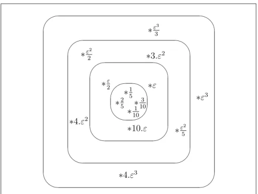
isomorphic to a cumulative algebra (Theorem 7), P is in fact a cumulative measure in the sense of Weydert [WEY 94]. In Fig. 1 is depicted an example of a pd-model
(without any valuation). The asterisks correspond to worlds and the numbers next to them represent their respective probabilities. The conceived worlds are the ones in the inner circle, the other worlds are surprising worlds. The other circles correspond to the global ranking of surprising worlds that was motivated in Sect. 1. This global ranking is closely related to Weydert’s notion of ranking and will be studied more in detail in Sect. 4. Note that both the sum of the probabilities of the conceived worlds and the global sum of all these worlds (conceived and surprising) are equal to 1 (see Sect. 1).
∗
ε3 3∗
ε2 2∗4.ε
3∗ε
3∗4.ε
2∗
ε2 5∗3.ε
2∗10.ε
∗
ε 2∗ε
∗
1 10∗
3 10∗
2 5∗
1 5 ' & $ % ' & $ % ' & $ % ' & $ %Figure 1. Example of a pd-model
2.1.2. Examples.
In this paper we will follow step by step two examples: the ‘Urn’ example and the ‘Answering Machine’ example of the introduction.
EXAMPLE9 (‘URN’ EXAMPLE). — Suppose the agent is in a fair, and there is an
urn containing n = 2.k > 0 balls which are either white or black. The agent does not know how many black balls there are in the urn but believes that it is equally probable that there are 0,1,..., or n black balls in the urn. Now say there is actually 0 black balls in the urn. This situation is depicted in Fig.2. The worlds are within squares and the double bordered world is the actual world. The numbers within squares stand for the probabilities of the worlds and the propositional letter pistands for: “there are i black
w0: p0,n+11 wi: pi,n+11 wn: pn,n+11
Figure 2. ‘Urn’ Example
2
EXAMPLE10 (‘ANSWERING MACHINE’ EXAMPLE). — Assume a professor (the
agent) comes back after lunch to her office. She ate with a colleague who just told her at lunch about his new timetable for this year. However she does not remember quite precisely what he said, in particular she is a bit uncertain whether his 1.5 hour lecture at 2.00 pm is on Tuesday or on Thursday, and she believes with probability4
5(resp. 15)
that his lecture is on Tuesday (resp. Thursday). In fact it is on Tuesday at 2.00 pm. We represent this situation in the model of Fig. 3. As in Fig. 2, the double bordered world is the actual world. The numbers within squares stand for the probabilities of the worlds and p (resp. ¬p) stands for “her colleague has his 1.5 hour lecture on Tuesday
(resp. Thursday)”2. 2
w : p,4
5 v : ¬p,15
Figure 3. ‘Answering Machine’ Example
2.1.3. Static language.
We can define naturally a language LStfor pd-models (St standing for Static).
DEFINITION11. — The syntax of the language LStis defined by
φ :=⊥| p | ¬φ | φ ∧ ψ | P (φ) ≥ x | Cφ where x ∈ [0; 1[, and p ranges over propositional letters.
Its semantics is inductively defined by M, w |= p iff w ∈ V (p);
M, w |= ¬φ iff not M, w |= φ
M, w |= φ ∧ ψ iff M, w |= φ and M, w |= ψ
2. Note that strictly speaking we would need two propositional variables p and p0, where p
(resp. p0) would stand for “her colleague has his lecture on Tuesday (resp.Thursday)” because
the fact that he does not have his lecture on Tuesday (¬p) should not imply logically that he has his lecture on Thursday (p0).
M, w |= P (φ) ≥ x iffP{P (v); M, v |= φ} ≥ x; M, w |= Cφ iffP{P (v); M, v |= φ} = 1.
M, w |= P (φ) ≥ x should be read “φ has a probability greater than x for the
agent”. (Note that the world w does not really play a role here.) M, w |= Cφ should be read “the agent is convinced (sure) of φ”. We use the term conviction instead of belief because the term “belief” refers in natural language to different concepts (that we distinguish here through LSt). Indeed, assume that you conjecture an arithmetical
theorem φ from a series of examples and particular cases. The more examples you have checked, the more you will “believe” in this theorem. This notion of belief corresponds to the type of formula P (φ) ≥ a for a real and smaller than 1; the bigger
a is the more you “believe” in φ. But if you come up with a proof of this theorem that
you have checked several times, you will still “believe” in this theorem but this time with a different strength. Your belief will be a conviction and corresponds here to the formula Cφ. However, note that this conviction (belief) might still be false if there is a mistake in the proof that you did not notice (like for Fermat’s theorem). Nevertheless, in the sequel we will alternatively and equivalently employ the terms “belief” and “conviction” for better readability. This notion of conviction actually corresponds to Lenzen’s in [LEN 78]. Moreover, if we define the operator B by M, w |= Bφ iff
M, w |= P (φ) > 0.5, then B corresponds to Lenzen’s notion of “weak belief” and C and B satisfy Lenzen’s axioms defined in [LEN 78]. This notion of conviction
also corresponds to Gärdenfors’ notion of accepted formula (in a belief set) [GäR 88]. This operator C satisfies the axioms K, D, 4, 5 but not the axiom T. So it does not correspond to the notion of knowledge and we do not deal with this notion in this paper. For a more in depth account on the different significations of the term “belief”, see for example [LEN 78].
Moreover, we can also express in this language what would surprise the agent, and how much. Indeed, in case x is an infinitesimal ε, P (φ) = ε should be read “the agent would be surprised with degree ε if she learnt that φ ”.3 (P (φ) = ε is defined
by P (φ) ≥ ε ∧ P (¬φ) ≥ 1 − ε.) Note that the smaller x is, the higher the intensity of surprise is. But this use of infinitesimals could also express how firmly we believe something, in Spohn’s spirit. Indeed, P (¬φ) = ε > ε0 = P (¬φ0) would then mean
that φ0is believed more firmly than φ.
Note that above, if x is real then only the conceived worlds have to be considered in the sumP{P (v); M, v |= φ} because the sum of any real (different from 0) with an
infinitesimal is equal to this real (see Sect. 1). Likewise, the semantics of C amounts to say that φ is true at least in all the conceived worlds of W . So it is quite possible to have a surprising actual world where ¬φ is true and still the agent being convinced of
φ (i.e. Cφ): just take φ:=“All swans are white” for example.
3. Note that this does not necessarily model all the things that would surprise the agent since there might still be things that the agent might conceive as possible with a low real probability and still be surprised to hear them claimed by somebody else (Gerbrandy, private communica-tion).
2.2. The dynamic part
2.2.1. The notion of generic action model
DEFINITION12. — A generic action model is a structure Σ = (Σ, S, P, {PΓ; Γ is a
maximal consistent subset of S }, {P reσ; σ ∈ Σ}, σ0) where
1) Σ is a finite set of possible actions; 2) σ0is the actual action;
3) S is a set of formulas of LStclosed under negation;
4) PΓis a probabilistic measure defined on P(Σ) indexed by each maximal
con-sistent subset Γ of S, and assigning to each possible action σ a real number in [0; 1]; 5) P is a probabilistic measure defined on P(Σ) and assigning to each possible action σ ∈ Σ a number in ]0; 1];
6) P reσis a function which takes as argument any propositional letter p and yields
a formula of LSt.
Intuitive interpretation. Items 1,2 are similar to Definition 8. It remains to give
an interpretation to items 3-6 of the definition.
Items 3 and 4. S corresponds to the set of facts about the world that are relevant
to determine the probabilities PΓof Item 4. The maximal consistent sets Γ then cover
all the relevant eventualities needed for the modelling. The choice of the formulas of
S is left to the modeler but they should be as elementary and essential as possible in
order to give rise to all the relevant eventualities. In that respect, one should avoid infinite sets S.
PΓ(σ) is the probability that the agent would expect (or would have expected) σ
to happen (among the possible actions of Σ), if the agent assumed that she was in a world where the formulas of Γ are true. In other words, PΓ(σ) can be viewed as the
probability for the agent that the action σ would occur in a world where the formulas of Γ are true. Note that this is a conditional probability of the form P (σ|Γ). Moreover, because we assume the agent to be rational, the determination of the value of this probability can often be done objectively and coincides with the agent’s subjective determination (see examples).
This probability value is real and cannot be infinitesimal (unlike P ), and (still un-like P ) we can have PΓ(σ) = 0. This last case intuitively means that the action σ
cannot physically be performed in a world where Γ is true. These operators PΓ
gen-eralize the binary notion of precondition in [BAL 04], [AUC 04] and [BEN 03].
REMARK 13. — In our definition of generic action model, instead of referring
di-rectly to worlds w of a particular pd-model, we refer to maximal consistent subsets Γ of a set S. This is for several reasons. Firstly, the determination of the probability
Pw(σ) does not depend on all the information provided by the world w but often on
might be performed in different situations, modelled by different pd-models, and be perceived differently by the agent in each of these situations, depending on what her epistemic state is (see Example 18). The use of maximal consistent sets enables us to capture this generic aspect of actions: in our very definition we do not refer to a particular pd-model. Finally, for computational reasons, we do not want that in prac-tice the definition of generic action models depends on a particular pd-model because we want to be able to iterate the action without having to specify at each step of the iteration the new action model related to the new pd-model. The use of maximal con-sistent sets allows us to do so. However, from now on and for better readability we note Pw(σ) := PΓ(σ) for the unique Γ such that M, w |= Γ (such a Γ exists
because S contains the negation of each formula it contains). 2 Item 5. P (σ) is the probability for the agent that σ actually occurs among Σ,
determined solely by the agent’s perception and observation of the action happening. This probability is independent of the agent’s beliefs of the static situation which could alter and modify this determination consciously or unconsciously (see the ‘answering machine’ example). This probability is thus independent of the probability that the agent would have expected σ to happen, because to determine this last probability the agent takes into account what she believes about the static situation (this fact will be relevant in Sect. 2.3).
Just as in the static case, we have conceived actions (which are assigned a real number) and surprising actions (which are assigned an infinitesimal). The former are actions that the agent conceives as possible candidates while one of the actions of Σ actually takes place. The latter are actions that the agent would be surprised to learn that they actually took place while one of the other actions took place. To take up the poker example of Sect. 2.1.1, if you play poker with somebody you trust and at a certain point he cheats while you do not suspect anything, then the actual action of cheating will be a surprising action for you (of value ε) whereas the action where nothing particular happens is a conceived action (of value 1). Just as in the static case, the relative strength of the actions (conceived and surprising) is expressed by the value of the operator P .
Item 6. The function P reσ deals with the problem of determining what facts
will be true in a world after the action σ takes place. Intuitively, P reσ(p) represents
the necessary and sufficient P recondition in any world w for p to be true after the performance of σ in this world w.
2.2.2. Examples
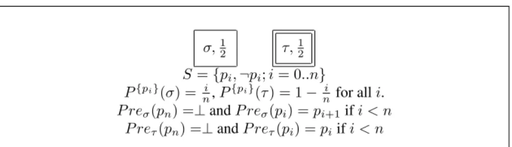
EXAMPLE 14 (‘URN’ EXAMPLE). — Consider the action whereby someone else
draws a ball from the urn (which is actually a white ball) and puts it in his pocket, the agent sees him doing that but she cannot see the ball. This action is depicted in Fig. 4. Action σ (resp. τ ) stands for “someone else draws a black (resp. white) ball and puts it in his pocket”. The numbers within the squares stand for the probabilities P (σ) of the possible actions. The maximal consistent sets are represented by their ‘positive’ components, so {pi} refers to the set {pi, ¬pk; k 6= i}.
σ,1 2 τ,12 S = {pi, ¬pi; i = 0..n} P{pi}(σ) = i n, P{pi}(τ ) = 1 −ni for all i. P reσ(pn) =⊥ and P reσ(pi) = pi+1if i < n P reτ(pn) =⊥ and P reτ(pi) = piif i < n
Figure 4. Someone else draws a (white) ball and puts it in his pocket and the agent is
uncertain whether he draws a white (σ) or a black ball (τ ).
The observation and perception of the action in itself does not provide the agent any reason to have a preference between him drawing a black ball or a white ball; so we set P (σ) = P (τ ) = 1
2.4 However if the agent assumed she was in a world
where there are i black balls then the probability that she would (have) expect(ed) him drawing a black (resp. white) ball would be i
n (resp. 1 −ni); so we set P{pi}(σ) = ni
and P{pi}(τ ) = 1 − i
n. Moreover there cannot be n black balls in the urn after he put
one ball in his pocket; so we set P reσ(pn) =⊥ and P reτ(pn) =⊥. But if he draws a
black ball then there is one black ball less; so we set P reσ(pi) = pi+1for all i < n.
Otherwise if he draws a white ball the number of black balls remains the same; so we set P reτ(pi) = pifor all i < n. 2
EXAMPLE 15 (‘ANSWERING MACHINE’ EXAMPLE). — Assume now that when
the professor enters her office, she finds a message on her answering machine from her colleague. He tells her that he will bring her back a book he had borrowed next Tuesday in the beginning of the afternoon between 2.00 pm and 4.00 pm. However, there is some noise on the message and she cannot distinguish precisely whether he said Tuesday or Thursday. Nevertheless she considers more probable of having heard Tuesday rather than Thursday.
We model this action in Fig. 5. σ stands for "her colleague says that he will come on Tuesday between 2.00 pm and 4.00 pm" and τ stands for "her colleague says that he will come on Thursday between 2.00 pm and 4.00 pm". P (σ) and P (τ ) represent the probabilities the agent assigns to σ and τ on the sole basis of what she has heard and distinguished from the answering machine (and are depicted within the squares). These probabilities are determined on the basis of her sole perception of the message. On the other hand, P{p}(σ) is the probability that she would have expected her
col-league to say that he will come on Tuesday (rather than Thursday) if she assumed that his lecture was on Tuesday. This probability can be determined objectively. Indeed, because we assume that her colleague has a lecture on Tuesday from 2.00 pm to 3.30 4. We could nevertheless imagine some exotic situation where the agent’s observation of him drawing the ball would give her some information on the color of the ball he is drawing. For example, if black balls were much heavier than white balls and the agent sees him having difficulty drawing a ball, she could consider more probable that he is drawing a black ball.
σ,3 5 τ,25 S = {p, ¬p}. P{p}(σ) = 1 5, P{p}(τ ) =45 P{¬p}(σ) = 4 5, P{¬p}(τ ) = 15. P reσ(p) = p, and P reτ(p) = p
Figure 5. The agent is uncertain whether her colleague says that he will come on
Tuesday (σ) or on Thursday (τ ) between 2.00 pm and 4.00 pm, but she considers more probable having heard Tuesday than Thursday.
pm, the only time he could come on Tuesday would be between 3.30 pm and 4.00 pm (only 0.5 hour). So we set P{p}(σ) = 0.5hr
2.5hrs = 15. Similarly, P{p}(τ ) = 2.5hrs2hrs = 45.
Finally, the message does not change the fact of her colleague having a lecture or not on Tuesday; so we set P reσ(p) = p and P reτ(p) = p.
2
2.3. The update mechanism 2.3.1. The notion of update product DEFINITION16. —
Given a pd-model M = (W, P, V, w0) and a generic action model Σ = (Σ, S, P, {PΓ; Γ
is a m.c. subset of S}, {P reσ; σ ∈ Σ}, σ0), we define their update product to be the
pd-model M ⊗ Σ = (W0, P0, V0, w0 0), where: 1) W0 = {(w, σ) ∈ W × Σ; Pw(σ) > 0}. 2) We set P0(σ) = P (σ).P W(σ) P {P (τ ).PW(τ ); τ ∈ Σ} where P W(σ) =X{P (v).Pv(σ); v ∈ W }. Then P0(w, σ) = P P (w) {P (v); v ∈ W and Pv(σ) > 0}.P 0(σ). 3) V0(p) = {(w, σ) ∈ W0; M, w |= P re σ(p)}. 4) w0 0= (w0, σ0).
Intuitive interpretation and motivations.
Items 1 and 4 As in BMS, in the new model we consider all the possible worlds
w, granted that this action σ can physically take place in w (i.e. Pw(σ) > 0). The
new actual world is the result of the performance of the actual action σ0in the actual
world w0.
REMARK 17. — When it comes to modelling epistemic states of agents, there are two (exclusive) approaches to follow: the objective approach and the subjective ap-proach. In the first approach, the modeler has an objective, external and omniscient knowledge of the agent’s epistemic state and the models she builds to represent the agent’s epistemic state are thus perfect and correct. This approach has applications in game theory (and economics) where an objective point of view is necessary to explain past economical behaviors for example. In the second approach, the modeler is the agent at stake herself and as such her perception of the situation might be erroneous because she is part of the situation. So the models she builds to represent her own epistemic state might be erroneous. This approach has applications in artificial intel-ligence where agents/robots need to have a formal representation of the surrounding world. These two approaches lead to two different kinds of formalism and ways to formalize belief change.
In this paper we follow the objective approach. With this assumption, our pd-models and generic action pd-models are correct. So the actual world and actual action of our models do correspond to the actual world and actual action in reality. It is then natural to assume that the actual action σ0 can physically be performed in the
actual world w0: Pw0(σ0) > 0. Hence, the existence of the (actual) world (w0, σ0) is
justified. 2
Item 2. We want to determine P0(w, σ) = P (W ∩ A), where W stands for the
event ‘we were in world w before σ occurred’ and A for ‘action σ just occurred’. More formally, in the probability space W0, W stands for {(w, τ ); τ ∈ Σ} and A
for {(v, σ); v ∈ W } and we can check that W ∩ A = {(w, σ)}. But of course to determine these probabilities we have to rely only on M and Σ.
Probability theory tells us that
P (W ∩ A) = P (W |A).P (A).
We first determine P (W |A), i.e. the probability that the agent was in world w
given the extra assumption that action σ occurred in this world. We reasonably claim
P (W |A) =P P (w)
{P (v); v ∈ W and Pv(σ) > 0}.
That is to say, we conditionalize the probability of w for the agent (i.e. P (w)) to the worlds where the action σ took place and that may correspond for the agent to the actual world w (i.e. {v; v ∈ W and Pv(σ) > 0}). That is the way it would be done
in classical probability theory. The intuition behind it is that we now possess the extra piece of information that σ occurred in w. So the worlds where the action σ did not
occur do not play a role anymore for the determination of the probability of w. We can then get rid of them and conditionalize on the remaining relevant worlds.
It remains to determine P (A), which we also denote P0(σ); that is to say the
probability for the agent that σ occurred. We claim that
P (A) = P1.P2
where P1is the probability for the agent that σ actually occurred, determined on
the sole basis of her perception and observation of the action happening; and P2 is
the probability that the agent would have expected σ to happen determined on the sole basis of her epistemic state (i.e. her beliefs). Because P1and P2are independent, we
simply multiply them to get P0(σ).
By the very definition of P (σ) (see Sect. 2.1), P1= P (σ).
As for P2, the agent’s epistemic state is represented by the worlds W . So she
could expect σ to happen in any of these worlds, each time with probability Pv(σ).
We might be tempted to take the average of them: P2 = P
{Pv(σ);v∈W }
n , where n is
the number of worlds in W . But we have more information than that on the agent’s epistemic state. The agent does not know in which world of W she is, but she has a preference among them, which is expressed by P . So we can refine our expression above and take the center of mass (or barycenter) of the Pv(σ)s balanced respectively
by the weights P (v)s (whose sum equals 1), instead of taking roughly the average (which is actually also a center of mass but with weights 1
n). We get P2= PW(σ) =
P
{P (v).Pv(σ); v ∈ W }. (Note that this expression could also be viewed as an
application of a theorem of conditional probability if we rewrote Pv(σ) to P (σ|v).)
Finally, we normalize P0(σ) on the set of actions Σ to get a probabilistic space.
We get
P (A) = P0(σ) = P P (σ).PW(σ)
{P (τ ).PW(τ ); τ ∈ Σ} where P
W(σ) =X{P (v).Pv(σ); v ∈ W }.
We can easily check thatP{P0(w, σ); (w, σ) ∈ W0} = 1, which ensures that P0
is a probability measure on P(W0).
Item 3. Intuitively, this formula says that a fact p is true after the performance of σ
in w iff the necessary and sufficient precondition for p to be true after σ was satisfied in w before the action occurred.5
5. In [AUC 05], the solution of determining which propositional facts were true after an up-date was very similar to Reiter’s solution to the frame problem [REI 01]. It turns out that the solution we propose here is equivalent to the previous one and was first proposed by Renardel De Lavalette [REN 04] and Kooi [KOO 05], [DIT 05]. Indeed, in [AUC 05] we used two oper-ators P ost+
σ and P ost−σ but in the update mechanism the necessary and sufficient condition for p to be true after σ was P ost+
2.3.2. Examples
EXAMPLE18 (‘URN’ EXAMPLE). — Assume now that someone else just drew a (white) ball from the urn and put it in his pocket, action depicted in Fig.4. Then because the agent considered equally probable that there was 0,1,..., or n black balls in the urn, she would expect that the other person drew a black ball or a white ball with equal probability. That is indeed the case:
PW(σ) =P{P (v).Pv(σ); v ∈ W } =P{ 1
n+1.ni; i = 0..n} =12 = PW(τ ).
Independently from that, her perception of the action did not provide her any rea-son to prefer σ over τ (i.e. P (σ) = P (τ )). So, in the end she should believe equally that the other agent drew a black ball or a white ball, and this is indeed the case:
P0(σ) = P0(τ ).
If we perform the full update mechanism, then we get the pd-model of Fig.6. In this model all the worlds are equally probable for the agent. Note that there cannot be
n black balls in the urn (pn) any longer since one of them has been withdrawn.
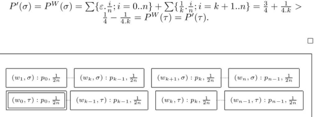
Now consider another scenario where this time the agent initially believes that there are more black balls than white balls (for example she believed somebody else that told her so in the beginning). This can be modelled by assigning the initial proba-bilities P (wi) = ε for i = 0, .., k and P (wi) = 1k for i = k + 1, .., n to the worlds of
the model depicted in Fig.1 (recall that there are n = 2.k balls). Then, if somebody else draws a ball from the urn and we compute again the probabilities of the actions σ and τ , we get what we expect, namely that the agent considers more probable that a black ball has been withdrawn rather than a white ball:
P0(σ) = PW(σ) =P{ε.i n; i = 0..n} + P {1 k.ni; i = k + 1..n} = 34+4.k1 > 1 4−4.k1 = PW(τ ) = P0(τ ). 2 (w1, σ) : p0,2n1 (wk, σ) : pk−1,2n1 (wk+1, σ) : pk,2n1 (wn, σ) : pn−1,2n1 (w0, τ ) : p0,2n1 (wk−1, τ ) : pk−1,2n1 (wk, τ ) : pk,2n1 (wn−1, τ ) : pn−1,2n1
Figure 6. Situation of the urn example after somebody else drew a white ball and put
it in his pocket (σ).
EXAMPLE19 (‘ANSWERING MACHINE’EXAMPLE). — Now that the professor has
heard the message, she updates her representation of the world with this new informa-tion. We are not going to perform the full update and display the new pd-model, but rather just concentrate on how she computes her action probabilities P0(σ) and P0(τ ).
After this computation, the probability P0(σ) that her colleague said that he will
come on Tuesday is a combination of: (1) how much she would have expected him to say so, based on what she knew and believed of the situation, and (2) what she actually distinguished and heard from the answering machine.
The first value (1) is PW(σ) = P{P (v).Pv(σ); v ∈ W }, and the second (2)
is P (σ). We get P0(σ) = 12
29 < 1729 = P0(τ ). The important thing to note here
is that σ has become less probable than τ for her: P0(σ) < P0(τ ) while before the
update P (σ) > P (τ ). On the one hand, this is due to the fact that the probability that she heard her colleague saying that he would come on Tuesday has decreased due to her lower expectation of him to say so: PW(σ) = 8
25 < 35 = P (σ); expectation
which is based on her belief that he is busy on Tuesday because he has got a lecture (P (p) = 4
5). On the other hand, this is due to the fact that the probability that she
heard her colleague saying that he would come on Thursday has increased due to her higher expectation of him to say so: P (τ ) = 2
5 < 1725= PW(τ )).
Now consider a second scenario where this time she initially believes with a higher probability that he has got a lecture on Thursday than on Tuesday (P (w) = 1
5 and
P (v) = 4
5 in Fig.2). This time her belief that she heard him saying that he will come
on Tuesday (resp. Thursday) is strengthened (resp. weakened) by her independent expectation of him to say so: P0(σ) > P (σ) > P (τ ) > P0(τ ).
2
EXAMPLE 20 (‘ANSWERING MACHINE’ EXAMPLE 2). — In this variant of the
answering machine example, we are going to show the usefulness of infinitesimals and show an example of belief revision.
Basically, we consider the same initial situation, except that her beliefs are differ-ent. This time she is convinced that her colleague’s lecture is on Thursday and she is also convinced that she heard him saying that he would come on Thursday. Formally, everything remains the same except that now in Fig. 3 P (w) = ε and P (v) = 1, and in Fig. 5 P (σ) = ε and P (τ ) = 1. If we apply the full update mechanism with these new parameters we get the model depicted in Fig. 7. In this model she is convinced that he has got a lecture on Thursday and that he said he would come on Thursday (world (v, τ )). Moreover, she would be surprised (with degree 5ε) if she learnt that her col-league has got his lecture on Tuesday or he said he will come on Tuesday (worlds (w, τ ), (v, σ) and (w, σ); remember that 5ε + 4ε2 = 5ε). But she would be much
more surprised (with degree ε2) if she learnt that he has got his lecture on Tuesday
and he said he will come on Tuesday (world (w, σ)), because that contradicts twice
her original convictions.
Now later her colleague tells her that he has got his lecture on Tuesday, then she will have to revise her beliefs. The action model of this public announcement is de-picted in Fig. 8. The resulting model is dede-picted in Fig. 9. In this model, she now believes that he has got his lecture on Tuesday, but she is still convinced that her colleague said that he will come on Thursday because no new information has contra-dicted this. This is made possible thanks to the (global) ranking of surprising worlds
(w, σ) : p, 4ε2 (w, τ ) : p, ε
(v, σ) : ¬p, 4ε (v, τ ) : ¬p, 1
Figure 7. Situation after she believed that her colleague’s lecture is on Thursday (¬p)
and she heard him saying that he would come on Thursday (τ ).
by infinitesimals. What happened during this revision process is that the least surpris-ing world where p is true became the only conceived world.
2
µ, 1 S = {p, ¬p} Pp(µ) = 1, P¬p(µ) = 0
P reσ(p) = p.
Figure 8. Her colleague announces to her that his lecture is on Tuesday.
((w, σ), µ) : p, 4ε ((w, τ ), µ) : p, 1
Figure 9. Situation after her colleague announced his lecture is on Tuesday (µ) and
she then revised her beliefs.
3. Extension to the multi-agent case.
In this section we only sketch a way to extend this framework to the multi-agent case. At the address ftp://ftp.irit.fr/IRIT/LILAC/Aucher_jancl.pdf can be found the detailed formalism. In the sequel, G is a fixed set of agents6.
6. Another possible and equivalent extension consists in simply indexing the probabilities PΓ
pd-We introduce a set of equivalence relations ∼jon the set of worlds W , modelling
the rough uncertainty of each agent j ∈ G. Then each ∼j equivalence class will be
considered as an instance of a “single-agent” pd-model with probability measure Pj
and should then fulfill the same conditions.
We do similarly for the generic action models by introducing a set of equivalence relations ∼jon the set of possible actions Σ indexed by the agents j ∈ G. Each ∼j
equivalence class will be considered as an instance of a “single-agent” generic action model with probability measures Pj and PjΓ and should fulfill the same conditions.
Moreover, we assume that the fact that an action cannot physically take place in a world is a public fact among agents. So we should add in the definition of the generic action model that for each possible action σ and agent j0, if PjΓ0(σ) = 0 then P
Γ j(σ) =
0 for all j ∈ G.
Finally, the update mechanism is the same as for the “single-agent” case: the P operators just have to be indexed by the agents j ∈ G. However we also have to deal with the new component ∼j. As in BMS, we set (w, σ) ∼0j (v, τ ) iff w ∼j v and
σ ∼j τ because the uncertainty relations ∼jfor the pd-model and the generic action
model are independent from one another.
4. Comparisons.
Structure of the static part and (its relevance for the) comparison with the AGM postulates. There are several proposals in the literature which cumulate fea-tures of ranking theories (Spohn-type or possibility theories) and probability: for ex-ample generalized qualitative probability [LEH 96], lexicographic probability [BLU 91], big-stepped probabilities [DUB 04] and Weydert’s cumulative algebra [WEY 94]. All these proposals are very similar in spirit and seem to be equivalent in one way or another. We showed in Theorem 7 that our structure V is actually an extension of a structure V0 isomorphic to a cumulative algebra. So Weydert’s comparisons with
Spohn’s theory [SPO 88] and possibility theories [DUB 91] transfer. In particular the ranking V0determines a global ranking of worlds similar in spirit to Spohn’s degrees
model (resp. generic action model) by the agents j ∈ G and possible worlds w (resp. possible actions σ) but allowing at the same time these probability measures to take the value 0 (note that it was not the case for the single-agent case). Pj,w(v) = 0 would then mean that if the
agent j is in world w then the world v is not relevant to describe her own epistemic state (and similarly for possible actions). However, if we want to have a framework equivalent to the first one, we have to add constraints to the Pj,w(and Pj,σ), namely
1) Pj,w(w) > 0 for all w ∈ W ,
2) if Pj,w(v) > 0 then for all u ∈ W Pj,w(u) = Pj,v(u),
3)P{Pj,w(v); v ∈ W } = 1.
Note that these constraints look similar to seriality (3), transitivity and euclidianity (2) con-straints. Finally, the update product is the same except that the probabilities P have to be replaced by Pj,w(or Pj,σ) and the probabilities PΓby PjΓ.
of disbelief or possibility degrees in possibility theory7. (The global degree of a world
w can be defined by α((P (w))0) ∈ P (w)0where α is a choice function; see the
ap-pendix.) So, more precisely our conceived worlds correspond to Spohn’s worlds of plausibility 0, and our surprising worlds correspond to Spohn’s worlds of plausibility strictly greater than 0; moreover our global degrees correspond to Spohn’s plausibility degrees (although the order has to be reversed). Likewise with possibility theory. In Fig. 1 of Sect. 2.1, the worlds with the same global degree are located between two consecutive spheres. But among the worlds of the same global degree exists also a
local ranking corresponding to the usual order relation. So for example, in the picture
we have the local ranking 4.ε2> 3.ε2, even if the worlds with these probabilities have
the same global degree.
As we saw in Sect. 2.1 this formalism allows an accurate and rich account of an epistemic state. Now we are going to see that its duality (local and global aspects) enables also a fine-grained account of its dynamics as well.
REMARK21. — In the literature (including myself in [AUC 04]), one often
consid-ers degrees of possibility/plausibility (present in possibility theory and Spohn’s the-ory) and probabilities as two different means to represent and tackle the same kind of information. However, as it is stressed in this paper, for us they are meant to model two related but different kinds of information. In our sense, the first rather corresponds to degrees of potential surprise about facts absent from the agent’s mind. The second rather corresponds to degrees of belief or acceptance about facts present (or acces-sible) in the agent’s mind (which can be a knowledge base for example). The same distinction is also present in [GäR 88]. 2
Our structure V is richer than the cumulative algebra V0 because it allows its
el-ements to have multiplicative inverses. This feature turns out to be quite useful in a dynamic setting because it allows conditionalization and in particular belief revision. THEOREM22. — If, as in the AGM theory, we restrict our attention to propositional
beliefs, then in the case of a public announcement our update mechanism satisfies the eight AGM postulates for belief revision.
Suppose φ is false in every conceived world, when we revise by φ then the sur-prising worlds where φ is true and which have the least global degree become the conceived worlds. More interestingly, the local structure of these surprising worlds remains the same, that is to say their relative order of probability is the same before and after the revision. So we see here that the richness of our formalism enables a fine-grained account of belief revision which is absent in the literature.
Comparison with Kooi’s system. Kooi’s dynamic probabilistic system [KOO 03] is based on the static approach by Fagin and Halpern in [FAG 94]. Unlike us, prob-ability is not meant only to model the agents’ epistemic states. In that respect, his
7. V0is defined as being the quotient structure of V0by the equivalence relation ≈0, which
is itself defined by x ≈0 y iff x
y is real different from 0 if y 6= 0 and x = 0 if y = 0 (see the
probability measures are defined relatively to each world without any constraint on them. Moreover he only deals with public announcement. But in this particular case our update mechanism is a bit different from his. The worlds of his initial model are the same as in his updated model, only the accessibility relations and probability dis-tributions are changed, depending on whether or not the probability of the formula announced is zero in the initial model. However, our probabilistic update rule in this particular case boils down to the same as his for the worlds where the probability of the formula announced is different from zero. Finally, he does not consider actions changing facts (he tackles this topic independently in [KOO 05]).
Comparison with van Benthem’s system. van Benthem’s early system [BEN 03] is similar to ours in its spirit and goals. However he does not introduce the probabilities
PW(σ) and P (σ) but only a single Pw(σ). Hence, his probabilistic update rule is
different. The intended interpretation of his Pw(σ) seems also to be different from
ours if we refer to his example. Anyway, his discussion and comparison with the Bayesian setting in his Sect. 5 are still valid here.
A more elaborated version of his system which is very similar to ours has been developed independently by him, Kooi and Gerbrandy [BEN 06]. In this system they do have a second probability measure P for the action models whose intended mean-ing is the same as ours. Nevertheless, their probabilistic update rule is still different and does not comply to the Jeffrey update, contrary to ours. They also study some parameterized versions of their probabilistic rule (which could be done here too) and they show that one of them actually complies to the Jeffrey update. They provide a sketch of a completeness proof via reduction axioms. However, they do not resort to infinitesimals to represent epistemic states and thus can neither express degrees of potential surprise nor allow for belief revision. Finally they do not consider actions changing facts.
Comparison with the situation calculus of Bacchus, Halpern and Levesque. Their system [BAC 99] can be viewed as the counterpart of van Benthem’s early sys-tem in the situation calculus except that they deal as well with actions changing facts. Their probabilistic update rule is also the same as van Benthem’s (modulo normaliza-tion). So what applies to van Benthem’s early system applies here too. In particular, the logical dynamics present in the interpretation of an action are not explored.
Comparison with the observation systems of Boutilier, Friedman and Halpern. Their system [BOU 98] deals with noisy observations. Their approach is semantically driven like ours. However they use a different framework called observation system based on the notion of (ranked) interpreted system. On the one hand their system is more general because it incorporates the notion of time and a ranking of evolutions of states over time (called runs). On the other hand the only actions they consider are noisy observations (which do not change facts of the situation). An advantage of our system is its versatility because we can represent many kinds of actions. In that re-spect, their noisy observations can be modelled in our framework using two possible actions, the first corresponding to a truthful observation and the second to an erro-neous one. Then by a suitable choice of probabilities we can for example express, as
they do, that the observation is “credible”. However, their framework seems to enable them to characterize formally more types of noisy observations. Finally, because we do not introduce the notions of time and history, our framework is rather comparable to a particular case of their system called Markovian observation system. But nothing precludes us to introduce these notions as an extension of our system.
5. Conclusion
In order to represent with most accuracy the agent’s epistemic state, we have in-troduced a rich formalism based on hyperreal numbers (and which is an extension of Weydert’s cumulative algebra). Our epistemic state representation includes both de-grees of beliefs expressed by a subjective probability and dede-grees of potential surprise expressed by infinitesimals. We have seen that the richness of this formalism enabled genuine belief revision thanks to the existence of infinitesimals (and multiplicative in-verse). By a closer look at this revision process, we could even notice some interesting and meaningful patterns due to the dual aspect (local and global) of this formalism. So, our system indirectly offers a new (probabilistic) approach to belief revision.
But other important logical dynamics were studied, namely the ones present in the process of interpreting an action. Starting from the observation that this interpre-tation hinges on two features, the actual perception of the action happening and our expectation of it to happen, we have proposed a way to model this phenomenon. In-cidentally, note that in a sense our approach complements and reverses the classical view whereby only our interpretation of actions affects our beliefs and not the other way around, as in belief revision theory. For sake of generality, we have also taken into account in this system actions that may change the facts of a situation.
Our system is semantically driven and it would be interesting to look for a com-pleteness result, and in particular for reduction axioms. However this system can be of use as it is in several areas. Firstly, in game theory where the kinds of phenomena we studied are quite current. Secondly, in psychology if we want to devise realistic formal models of belief change. Finally, the logical dynamics we modelled could be used in some way or another in artificial intelligence since they are the hallmark of rational and efficient reasoners.
Acknowledgements
First of all, I thank my PhD supervisors Hans van Ditmarsch and Andreas Herzig for many useful comments and discussions. I also thank Didier Dubois for endless conversations that showed me (among other things) the connections of my formalism to represent the agent’s epistemic state to other formalisms. I thank Jérôme Lang for suggesting the second extension to the multi-agent case. I thank three anonymous referees for their comments to improve the presentation. Finally, I thank the audiences of the workshop “belief revision and dynamic logic” at ESSLLI05 and of the Dagstuhl
Seminar “belief change in rational agents: perspectives from artificial intelligence, philosophy, and economics” for their attention, questions and comments.
6. References
[ADA 75] ADAMSE. W., The Logic of Conditionals, vol. 86 of Synthese Library, Springer,
1975.
[AUC 04] AUCHERG., “A Combined System for Update Logic and Belief Revision”, BAR
-LEYM., KASABOVN. K., Eds., Intelligent Agents and Multi-Agent Systems, 7th Pacific
Rim International Workshop on Multi-Agents (PRIMA 2004), vol. 3371 of LNCS, Springer,
2004, p. 1–17, Revised Selected Papers.
[AUC 05] AUCHER G., “How Our Beliefs Contribute to Interpret Actions.”, PECHOUCEK
M., PETTAP., VARGAL. Z., Eds., Multi-Agent Systems and Applications IV, 4th
Interna-tional Central and Eastern European Conference on Multi-Agent Systems (CEEMAS 2005),
vol. 3690 of LNCS, Springer, 2005, p. 276–285.
[BAC 99] BACCHUSF., HALPERN J., LEVESQUEH., “Reasoning about Noisy Sensors and Effectors in the Situation Calculus”, Artificial Intelligence, vol. 111, num. 1-2, 1999, p. 171–208.
[BAL 98] BALTAGA., MOSS L., SOLECKIS., “The logic of Common Knowledge, Public
Announcement, and Private Suspicions”, GILBOAI., Ed., Proceedings of the 7th
confer-ence on theoretical aspects of rationality and knowledge (TARK98), 1998, p. 43–56.
[BAL 04] BALTAGA., MOSSL., “Logic for Epistemic Program”, Synthese, vol. 139, num. 2,
2004, p. 165–224.
[BEN 03] VAN BENTHEM J., “Conditional Probability Meets Update Logic.”, Journal of
Logic, Language and Information, vol. 12, num. 4, 2003, p. 409–421.
[BEN 06] VANBENTHEMJ., GERBRANDYJ., KOOIB., “Dynamic Update with Probability”, report , march 2006, ILLC.
[BLU 91] BLUME L., BRANDENBURGERA., DEKEL E., “Lexicographic Probabilities and
Choice under Uncertainty”, Econometrica, vol. 59, num. 1, 1991, p. 61–79.
[BOU 98] BOUTILIER C., HALPERN J., FRIEDMAN N., “Belief Revision with Unreliable Observations”, Proceedings of the Fifteenth National Conference on Artificial Intelligence
(AAAI 1998), 1998, p. 127–134.
[DIT 05] VAN DITMARSCH H. P., VAN DER HOEK W., KOOI B. P., “Dynamic epistemic logic with assignment.”, DIGNUMF., DIGNUMV., KOENIGS., KRAUSS., SINGHM. P.,
WOOLDRIDGEM., Eds., AAMAS, ACM, 2005, p. 141–148.
[DUB 91] DUBOISD., PRADE H., “Possibilistic Logic, Preferential Model and Related Is-sue”, Proceedings of the 12th International Conference on Artificial Intelligence (IJCAI), Morgan Kaufman, 1991, p. 419–425.
[DUB 04] DUBOISD., FARGIERH., “A Unified Framework for Order-of-Magnitude Confi-dence Relation”, Twentieth Conference in Artificial Intelligence, 2004, p. 138–145. [FAG 94] FAGINR., HALPERNJ., “Reasoning about Knowledge and Probability”, Journal of
[GäR 88] GÄRDENFORSP., Knowledge in Flux (Modeling the Dynamics of Epistemic States),
Bradford/MIT Press, Cambridge, Massachusetts, 1988.
[KEI 86] KEISLER H. J., Elementary Calculus: an Approach Using
Infinitesi-mals, Prindle and Weber & Schmidt, 1986, Online edition on the website http://www.math.wisc.edu/ keisler/calc.html.
[KOO 03] KOOIB., “Probabilistic Dynamic Epistemic Logic”, Jourbal of Logic, Language
and Information, vol. 12, num. 4, 2003, p. 381–408.
[KOO 05] KOOIB., “As the World Turns: On the Logic of Public Update”, Manuscript, 2005. [LEH 96] LEHMANND., “Generalized Qualitative Probability: Savage Revisited”, HORVITZ
E., JENSENF., Eds., Twelfth Conference on Uncertainty in Artificial Intelligence, Portland, Oregon, August 1996, Morgan Kaufmann, p. 381–388.
[LEN 78] LENZENW., Recent Work in Epistemic Logic, Acta Philosophica 30, North Holland Publishing Company, 1978.
[REI 01] REITER R., Knowledge in Action: Logical Foundations for Specifying and
Imple-menting Dynamical Systems, MIT Press, 2001.
[REN 04] RENARDELDELAVALETTEG. R., “Changing Modalities”, Journal of Logic and
Computation, vol. 14, num. 2, 2004, p. 251–275.
[SPO 88] SPOHN W., “A General Non-Probability Theory of Inductive Reasoning”,
SCHACHTERR., LEVITTT., KANALL., LEMMERJ., Eds., Uncertainty in Artificial
Intel-ligence 4, North-Holland, 1988, p. 149–158.
[WEY 94] WEYDERT E., “General Belief Measure”, DE MÁNTARAS R. L., POOLED., Eds., Tenth Conference on Uncertainty in Artificial Intelligence, Morgan Kaufmann, 1994, p. 575–582.
A. Proof of Theorem 3., Lemma 5. and Theorem 6.
THEOREM23 (THEOREM3.). — The quotient structure V = (∗R+/
≈, +, .) is a
semi-field.
PROOF. — We only need to prove that + and . are well defined, since the rest is
standard and straightforward.
Assume x = x0and y = y0. We have to show x+y = x0+y0and x.y = x0.y0.
First, let us show that x+y = x0+y0.
Assume x = 0 (similar proof for y = 0). Then x = x0 = 0. In that case
x+y = x + y = y = y0= 0 + y0 = x0+ y0 = x0+y0.
Assume x 6= 0 and y 6= 0. Then x, x0, y, y0are all different from 0. So x + y 6= 0
x+y = x0+y0iff
x + y = x0+ y0iff
St(xx+y0+y0) = 1 because x + y 6= 0 (see above) iff
St( x x+y) + St( y0 x+y) = 1 iff St(x0 x.1+1y x) + St( y0 y.1+1x y) = 1 iff St(x0 x).St(1+1yx) + St( y0 y).St(1+1x y) = 1 iff St( 1 1+y x) + St( 1 1+x y) = 1 because St( x0 x) = St( y0 y) = 1 iff 1 1+St(y x)+ 1 1+St(x y) = 1 iff 1 1+St(y x)+ 1 1+ 1 St( yx) = 1 which is true.
Now, let us show that x.y = x0.y0.
Assume x = 0 (similar proof for y = 0). Then x = x0 = 0 and the equality is
fulfilled.
Assume x 6= 0 and y 6= 0. Then x, x0, y, y0are different from 0. So x.y 6= 0.
x.y = x0.y0iff
x.y = x0.y0iff
St(xx.y0.y0) = 1 because x.y 6= 0 iff
St(x0 x).St( y0 y) = 1 iff 1.1 = 1 which is true. n LEMMA24 (LEMMA5.). — If x / y then for all x0∈ x and all y0∈ y, x0 ≤ y0.
PROOF. —
1) Assume x 6= 0 and y 6= 0 (then x, y are different from 0). a) If x = y then we have the result.
b) If x 6= y then by definition there are x0∈ x and y0∈ y such that x0< y0.
- Assume that either x0 ≤ y0 ≤ x0 ≤ y0 or x0 ≤ y0 ≤ y0 ≤ x0 or x0≤ y0≤ y0 ≤ x0. Then x0≤ y0 ≤ x0, so x0 x0 ≤ y0 x0 ≤ x0 x0 because x06= 0, then 1 ≤ St(xy0 0) ≤ St( x0 x0) = 1 because x 0, x 0∈ x, then St(y0 x0) = 1, y0∈ x 0= x,
x = y0 = y which is impossible by assumption.
- Assume that either y0 ≤ x
0 ≤ x0 ≤ y0 or y0 ≤ x0 ≤ x0 ≤ y0 or y0 ≤ x 0≤ y0≤ x0. Then y0 ≤ x 0≤ y0, then y0 y0 ≤ x0 y0 ≤ 1 because y06= 0, then 1 = St(yy0 0) ≤ St( x0 y0) ≤ 1, then St(x0 y0) = 1, then
x = x0= y0= y which is impossible by assumption.
So in all possible cases we reach a contradiction. This means that for all x0∈ x,
all y0∈ y x0 ≤ y0
2) a) If x = 0 and y 6= 0, then
0 / y then there is y0∈ y such that 0 < y0.
Assume there is y0∈ y such that 0 > y0. Then
y0< 0 ≤ y 0 y0 y0 < 0 ≤ y0 y0 = 1 1 = St(y0 y0) ≤ 0 ≤ 1 because y 0, y 0∈ y
i.e. 0 = 1, which is counterintuitive.
So for all y0∈ y, 0 ≤ y0.
b) if y = 0 and x 6= 0 then
x ≤ 0, so there is x0∈ x such that x0< 0.
Assume there is x0∈ x such that x0 > 0.