HAL Id: hal-00590600
https://hal.archives-ouvertes.fr/hal-00590600
Submitted on 4 May 2011
HAL is a multi-disciplinary open access archive for the deposit and dissemination of sci-entific research documents, whether they are pub-lished or not. The documents may come from teaching and research institutions in France or abroad, or from public or private research centers.
L’archive ouverte pluridisciplinaire HAL, est destinée au dépôt et à la diffusion de documents scientifiques de niveau recherche, publiés ou non, émanant des établissements d’enseignement et de recherche français ou étrangers, des laboratoires publics ou privés.
Najib Mohamed Najid, Marouane Selsouli Alaoui, Abdelmoula Mouhafid
To cite this version:
Najib Mohamed Najid, Marouane Selsouli Alaoui, Abdelmoula Mouhafid. An Integrated Production and Maintenance Planning Model with time windows and shortage cost. International Journal of Production Research, Taylor & Francis, 2010, pp.1. �10.1080/00207541003620386�. �hal-00590600�
For Peer Review Only
An Integrated Production and Maintenance Planning Model with time windows and shortage cost
Journal: International Journal of Production Research Manuscript ID: TPRS-2009-IJPR-0370.R1
Manuscript Type: Original Manuscript Date Submitted by the
Author: 21-Oct-2009
Complete List of Authors: Najid, Najib; Université de Nantes/IRCCyN, IUT de Nantes, Dep. GMP, 2, rue du Prof Jean Rouxel, 44475
Alaoui, Marouane; Université de Nantes/IRCCyN, Ecole des mines de Nantes, 4 rue Alfred Kastler BP 20722 F- 44307 Nantes cedex 3 France
Mouhafid, Abdelmoula; Université de Nantes/IRCCyN, IUT de Nantes, Dep, QLIO, 2, rue du Prof. Jean Rouxel, 44475 Keywords: LOT SIZING, MAINTENANCE PLANNING
Keywords (user): time windows, shortage cost
For Peer Review Only
An Integrated Production and Maintenance Planning Model with
time windows and shortage cost
Najib .M. Najid*
Université de Nantes, Nantes Atlantique, IRCCyN
IUT de Nantes, Dep. GMP
2, avenue du Peof Jean Rouxel
B.P. 539- 44475 Carquefou, France
Email : najib.najid@univ-nantes.fr
Tel. 00 33 2 28 09 20 94
Fax. 00 33 2 28 09 20 21
Marouane Alaoui-Selsouli
Université de Nantes, Nantes Atlantique, IRCCyN
Ecole des Mines de Nantes
4, rue Alfred Kastler
B.P. 20722F-44307 Nantes cedex France
Email : malaou07@emn.fr
Tel. 00 33 2 28 09 20 17
Fax. 00 33 2 28 09 20 21
Abdelmoula Mohafid
Université de Nantes, Nantes Atlantique, IRCCyN
IUT de Nantes, Dep. QLIO
2, avenue du Peof Jean Rouxel
B.P. 539- 44475 Carquefou, France
Email : abdelmoula.mohafid@univ-nantes.fr
Tel. 00 33 2 28 09 21 22
Fax. 00 33 2 28 09 20 21
*Corresponding author 3 4 5 6 7 8 9 10 11 12 13 14 15 16 17 18 19 20 21 22 23 24 25 26 27 28 29 30 31 32 33 34 35 36 37 38 39 40 41 42 43 44 45 46 47 48 49 50 51 52 53 54 55 56 57 58 59 60For Peer Review Only
An Integrated Production and Maintenance Planning Model with
time windows and shortage cost
Abstract: In this paper, we tackle the problem of integrating production and maintenance. Production problem addresses the issue of determining the production lot sizes of various items. Preventive maintenance is carried out in time windows to restore the production line to an ‘as-good-as-new’ status, and when a production line fails, a minimal repair is carried out to restore it to an ‘as-bad-as-old’ status. The resulting problem is modelled as a linear mixed-integer program. It takes into account demand shortage and the reliability of the production line. Computational experiments are carried out to show the effectiveness of the integrated model compared to classical separate model for different instances, and the obtained results are analyzed in detail.
Keywords: Production and maintenance planning, Time windows, Shortage cost.
1.
Introduction
In the industrial environment, the relationship between production and maintenance has been conflictual in nature. This attitude is perpetuated by the lack of communication regarding the scheduling requirements of each function. Maintenance is generally a secondary process in companies that have production as their core business. Production management often views maintenance in the context of hours or days out of service and fails to realize the strategic importance of incorporating maintenance in the manufacturing planning. On the other hand, management for the maintenance function attempts to impose constraints on production that it deems necessary to achieve complete equipment reliability. The result is that the implementation of an optimal maintenance policy is constrained by the demands of production.
Currently, production planning and maintenance are performed separately. For instance, common ERP modules include production planning module that optimizes the utilization of manufacturing capacity, parts, components and material resources. Maintenance module is a peripheral module little known in fact, it is not part of core ERP application as production planning, finance, HR (Human Resources) Modules. it is considered as computerized maintenance management system (CMMS), and it allows managing preventive and corrective maintenance of all material assets of the company. We notice that each of these modules is used independently with specific data from each service, and no coordination is implemented to reduce production and maintenance costs. Therefore, maintenance planning should be an integral part of the overall business strategy and should be coordinated and scheduled with manufacturing activities. So, we should consider maintenance as integral parts of the production plan rather than as interruptions to that plan. Any violation of the maintenance schedule is treated as a violation of the production plan integrity.
3 4 5 6 7 8 9 10 11 12 13 14 15 16 17 18 19 20 21 22 23 24 25 26 27 28 29 30 31 32 33 34 35 36 37 38 39 40 41 42 43 44 45 46 47 48 49 50 51 52 53 54 55 56 57 58 59 60
For Peer Review Only
To solve this problem, we develop an integrated production planning and maintenance activities. This integration hedge against often avoidable failures and re-planning occurrences, and minimize loss of demand which is not without consequence for companies. In this area, we propose an integrated model of production and maintenance planning that minimizes production, inventory, set up, demand shortage, preventive and corrective maintenance costs. The particularity of our model is that preventive maintenance actions are planned in time windows, and demand shortage is allowed when the resource capacity is not sufficient to meet all demand.
The remainder of the paper is organized as follows. In the second section a brief literature review is presented. In the third section, we describe separate production planning and maintenance problem, and we state its mathematical formulation. We illustrate our integrated problem in the fourth section. Computational results are showed in the fifth section, and we end up with conclusion and outlooks in the last section.
2.
Brief literature review
The problem of joint planning of production and maintenance is a recent problem tackled in research due to its importance in the current highly competitive environment. Several relations exist in different ways between maintenance and production according to Budai and al. (2006). First of all, when planning maintenance takes into account production (e.g. Dekker and Van Rijn. (1996); BÄackert and Rippin. (1985); Cassady and al. (2001), Marquez and al. (2003). Secondly , maintenance can also be seen as a production process which needs to be planned, see e.g. Dijkstra and al, (1994). Shenoy and Bhadury. (1993), Rosheil and Christy (1996), Yan and al. (2004). Finally, the integrated models of production and maintenance which we are interested in our research work.
Several studies of integrated production planning and maintenance problem were proposed with different approaches, resolution methods, and modeling tools. In the literature, we find models developed with stochastic aspect by using such Markov chains to oversee the state of machine or to determine an optimal buffer level according to the production rate in order to establish an interdependent policy of maintenance and production. In the last decade, large models were stated in this context, some of them treat the control problem of a stochastic manufacturing system with random breakdowns, repairs and preventive maintenance. The objective of the control models is to find the production and the preventive maintenance rates of the machines so as to minimize the total cost of inventory/backlog, repair and preventive maintenance see e.g. Kenné and Boukas (2003), Kenné and Gharbi (2004), Gharbi and Kenné (2005), and Rezg and al. (2005). An extension was proposed by Charlot and al. (2007) considering preventive maintenance activities and differentiates two types of repairs: repairs
3 4 5 6 7 8 9 10 11 12 13 14 15 16 17 18 19 20 21 22 23 24 25 26 27 28 29 30 31 32 33 34 35 36 37 38 39 40 41 42 43 44 45 46 47 48 49 50 51 52 53 54 55 56 57 58 59 60
For Peer Review Only
with lockout/tagout, associated with accident prevention, and repairs without lockout/tagout. Other research works deal with models of production systems with buffer inventory. The role of this buffer inventory is to satisfy demand when corrective or preventive maintenance is carried out. One of the earliest and basis work on this subject is Van der Duyn Schouten and Vanneste (1995). In their model the demand rate is constant and equal to d (units/time) and as long as the fixed buffer capacity (K) is not reached the installation operates at a constant rate of p units/time (p > d) and the excess output is stored in the buffer. When the buffer is full, the installation reduces its speed from p to d. Upon failure corrective maintenance starts and the installation becomes as good as new. The decision to start a preventive maintenance action is not only based on the condition of the installation, but also on the level of the buffer. The criterion to minimize is the average inventory level and the average number of backorders. Iravani and Duenyas (2002) extended the above model by assuming a stochastic demand and production process. Kyriakidis and Dimitrakos (2006) studied an infinite-state generalization of Van der Duyn Schouten and Vanneste (1995). Preventive maintenance actions can be regularly (after each T time periods) performed and the duration of corrective and preventive maintenance actions is random see e.g Chelbi and Ait KAdi(2004), and the possibility of imperfect production can be included in model for example Zequeria and al. (2004). Dhouib and al. (2008) worked on production lines composed of several serial machines which are subject to random operation-dependent failures when it has no intermediate buffers between adjacent machines. Models of preventive maintenance policy with control quality of products for a randomly failing production system producing conforming and non-conforming units can be developed e.g, Radhoui and al. (2009). The considered system consists of one machine designed to fulfill a constant demand. According to the proportion l of non-conforming units observed on each lot and compared to a threshold value lm, one decides to undertake or not maintenance actions on the system.
A continuous time models with an infinite time horizon were presented such economic manufacturing quantity (EMQ) models with failure aspects. The study of those models is based on failures of production system and their impacts on the decisions of the lot sizing, see e.g. Groenevelt and al (1992) who consider the effects of stochastic machine breakdowns and corrective maintenance on economic lot sizing decisions, and propose to use the EMQ as an approximation to the optimal production lot size. Chung (2003) provides a better approximation to the optimal production lot size, Makis and Fung (1995) proposed a model for joint determination of the lot size, inspection interval and preventive replacement time for a production facility that is subject to random failure. Srinivasan and Lee (1996) considered an (S, s) policy, i.e. as soon as the inventory level reaches S, a preventive maintenance operation is initiated and the machine becomes as good as new. After the preventive
3 4 5 6 7 8 9 10 11 12 13 14 15 16 17 18 19 20 21 22 23 24 25 26 27 28 29 30 31 32 33 34 35 36 37 38 39 40 41 42 43 44 45 46 47 48 49 50 51 52 53 54 55 56 57 58 59 60
For Peer Review Only
maintenance operation, production resumes as soon as the inventory level drops down to or below a prespecified value s, and the facility continues to produce items until the inventory level is raised back to S. If the facility breaks down during operation, it is minimally repaired and put back into commission.
Unlike the above mentioned continuous time models, the discrete time models assume that the planning horizon is finite and divided into discrete periods for which demand is given and may vary between periods. A few works exist in this area, they concern aggregate production planning problems known as multi items capacitated lot sizing problems at which, we integrate decision variables modeling preventive and corrective maintenance. To our knowledge, the only works developed within this framework are proposed by Weinstein and Chung (1999), Aghezzaf and al. (2007), and Aghezzaf and Najid (2008). Weinstein and Chung (1999) presented a three part-model to resolve the conflicting objectives of system reliability and profit maximization. An aggregate production plan is first generated, and then a master production schedules is developed to minimize the weighted deviations from the specified aggregate production goals. Finally, work-center loading requirements, determined through rough cut capacity planning, are used to simulate equipment failures during the aggregate planning horizon. Aghezzaf and al. (2007) studied a production system that subjects to random failures. They assume that any maintenance action carried out on the system, in a period, reduces the system’s available production capacity during that period. The objective is to find an integrated lot-sizing and preventive maintenance strategy of the system that satisfies the demand for all items over the entire horizon without backlogging, and which minimizes the expected sum of production and maintenance costs. An extension of the above work is treated by Aghezzaf and Najid (2008). They developed models which take into consideration the parameters of reliability of the system and consider parallel production lines. Our motivation by this paper is to provide an extension of these models to a more complete and more flexible model in relation to the date of preventive maintenance tasks. The aim of our study is to establish a joint production and maintenance planning problem at the tactical level to minimize the total costs associated with production and maintenance. Before describing our problem, we will define both of aggregate production and maintenance planning.
3.
Statement of the separate problem
3.1
Maintenance problem
Throughout their operational life, complex industrial systems are subject to corrective operations and preventive maintenances to keep them in working order. Preventive maintenance is a schedule of planned maintenance actions aimed at the prevention of
3 4 5 6 7 8 9 10 11 12 13 14 15 16 17 18 19 20 21 22 23 24 25 26 27 28 29 30 31 32 33 34 35 36 37 38 39 40 41 42 43 44 45 46 47 48 49 50 51 52 53 54 55 56 57 58 59 60
For Peer Review Only
breakdowns and failures. The primary goal of preventive maintenance is to prevent equipment failure before it actually occurs. Corrective maintenance is defined as maintenance work which involves the repair or replacement of components which have failed or broken down. Maintenance problem is to answer the question: when do we perform preventive maintenance task, ie, what is the periodicity of preventive maintenance?
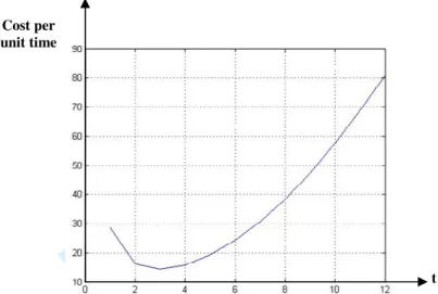
Several policies have been proposed to address this issue, the readers can refer to Wang (2002) for a detailed review of these policies. Initially, in our policy the preventive
maintenance actions are performed at fixed time intervals k (k=1, 2 …), and corrective
maintenance actions are carried out at failures occurs. Then, we have to determine the optimal
length of preventive maintenance period which minimizes the expected maintenance cost
per unit time (example, see figure 1).
Parameters:
: Preventive maintenance cost. : Corrective maintenance cost.
: Preventive maintenance period (periodicity). : Optimal preventive maintenance period.
: Failure rate function.
: Number of preventive maintenance during the horizon.
: Expected number of failures during .
: Expected corrective maintenance cost between [t1, t2]
: Expected maintenance cost for a period t.
: Expected cost per unit time of maintenance Gertsbakh, (2000).
: Expected total cost of maintenance throughout a finite time horizon
.
[Insert figure 1 here]
3 4 5 6 7 8 9 10 11 12 13 14 15 16 17 18 19 20 21 22 23 24 25 26 27 28 29 30 31 32 33 34 35 36 37 38 39 40 41 42 43 44 45 46 47 48 49 50 51 52 53 54 55 56 57 58 59 60
For Peer Review Only
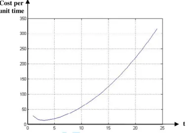
We consider in this paper a finite time horizon of length T. Once, the length of preventive maintenance period is known, we compute the expected total maintenance cost throughout the horizon which is based on the expected maintenance cost per preventive
maintenance period and ( ) (example, see figure 2)1.
[Insert figure 2 here]
The mathematical formulation of the expected total maintenance cost throughout the horizon is given below:
We implement an algorithm to compute preventive maintenance period and all the costs described above including the calculation of the expected total maintenance cost CT in a finite horizon. This cost is important to compare a separate study of the problem with our integrated one in computational results in the following section. The algorithm is stated as follows:
Algorithm
Initialization:
Parameters of the used failure distribution; Preventive maintenance cost;
Corrective maintenance cost; Main program:
for t = 1: to Number_period do
Computation of expected number of failures in each period t (NB(t)).
Computation of expected maintenance (preventive and corrective) cost in each
period t ( ).
Computation of expected maintenance cost per unit time in each period t (equation (1)).
End for
Determination of the optimal result .
Computation of expected maintenance cost per preventive maintenance period
1
Note that if CT will dependent only on . 3 4 5 6 7 8 9 10 11 12 13 14 15 16 17 18 19 20 21 22 23 24 25 26 27 28 29 30 31 32 33 34 35 36 37 38 39 40 41 42 43 44 45 46 47 48 49 50 51 52 53 54 55 56 57 58 59 60
For Peer Review Only
Computation of expected total maintenance cost throughout the horizon (equation (2) or (3))
3.2
Aggregate production planning
A production plan establishes resource requirements to perform processing from raw material to finished products, in order to satisfy customers in the most efficient and most economical possible way. In other words, decisions to produce are made in the best report between the financial objective and the one of customer satisfaction.
The basis of our work is the multi items capacitated lot sizing problems which are the main production planning problems with setups between production lots. Because of these setups, it is often too costly to produce a given product in every period. On the other hand, generating fewer setups by producing large quantities to satisfy future demands results in high inventory holding costs. Thus, the objective is to determine the periods where production should take place, and the quantities to be produced, in order to satisfy demand while minimizing production, setup and inventory holding costs. Other costs might also be considered, examples are backorder cost, backlogging cost, shortage cost etc. In our work, we will consider shortage cost. To our knowledge, there are few works that deal with lots sizing problems with demand shortage. Sandbothe and Thompson (1990) and Aksen and al. (2003) addressed a single item lot sizing problem with constant capacity and shortage cost. Absi and kedad (2008) dealt with a multi item capacitated lot sizing problem with shortage cost, and an extension to a multi-item capacitated lot-sizing problem with setup times , safety stock and demand shortage Absi and kedad (2009). For more information about multi items capacitated lot sizing problems, the reader can refer to a detailed review presented by Karimi and al. (2003).
Let define the parameters and the mathematical formulation of the multi items
capacitated lot sizing problem with demand shortage denoted (MCLSP-SC) below:
Index: P : set of item. T : set of period. i : Items. t : Periods. Model parameters:: Demand of item i to satisfy during period t.
: Set-up cost of producing one unit of item i in period t. : Fixed cost of producing one unit of item i period t.
3 4 5 6 7 8 9 10 11 12 13 14 15 16 17 18 19 20 21 22 23 24 25 26 27 28 29 30 31 32 33 34 35 36 37 38 39 40 41 42 43 44 45 46 47 48 49 50 51 52 53 54 55 56 57 58 59 60
For Peer Review Only
: Variable cost of holding one unit of item i by the end of period t.: Unit cost for requirements not met regarding demand for item i in period t. : Processing time for each item i.
: Capacity consumed by preventive maintenance action in period t. (t) : Capacity consumed by corrective maintenance action in period t.
: Vector of N (Number of period) elements contains the expected number of failures NB(t) in each period t of horizon if we don’t perform any preventive maintenance action (figure 5).
K (t) : Available capacity in period t.
=
Decision variables:
: Binary set up variable of item i in period t. : Quantity of item i produced in period t. : Inventory of item i at the end of period t. : Demand shortage for item i in period t. : Binary preventive maintenance variable.
MCLSP-SC:
Subject to:
3 4 5 6 7 8 9 10 11 12 13 14 15 16 17 18 19 20 21 22 23 24 25 26 27 28 29 30 31 32 33 34 35 36 37 38 39 40 41 42 43 44 45 46 47 48 49 50 51 52 53 54 55 56 57 58 59 60
For Peer Review Only
The objective function (4) minimizes the sum of the set up, holding, production, demand shortage costs over the whole N-period horizon. Constraint (5) is the inventory balance equation. Constraint (6) is the capacity constraint where preventive maintenance actions and expected number of breakdowns in each period are known. Constraint (7) relates the continuous production variables to the binary setup variables. Constraint (8) expresses that quantity lost of item i in period t must be less than demand of item in period t. The constraints (9) and (10) express non-negativity and integrality constraints.
The multi items capacitated lot sizing problem often has been studied in literature. Solution methods of the problem can be classified into three main categories. The first is exact methods e.g Barany et al. (1984), Eppen and Martin (1987), the second category is common-sense or specialized heuristics e.g Maes and Van Wassenhove (1988), Kirca and Kokten (1994,) Karni and Roll (1982) and the third category belong to mathematical programming-based heuristics e.g. Thizy and Van Wassenhove (1985), Trigeiro(1987), Diaby et al. (1992). There are few references dealing with lot-sizing problems with shortage costs. . Absi and kedad (2008) used inequalities within a branch-and-cut framework to find near optimal solutions, and Absi and kedad (2009) developed a Lagrangian relaxation of the capacity constraints to obtain lower and upper bounds for their problem. To the best of our knowledge, there are the first papers that deal with shortage costs for the multi-item capacitated lot-sizing problem.
Let the total cost of maintenance and production in the separate study, it will
be the sum of expected total cost of maintenance throughout a finite time horizon
CT
(determined in section 3.1)
and the optimal cost obtained from MCLSP-SC model .4. Integrated production planning and maintenance problem
Consider a planning horizon H of length covering N periods of fixed length ,
and a set of item to be produced on a capacitated production line. During each
period , a demand of item should be satisfied. Items are produced on a
production line with known capacities given in unit time, and processing time expressed in unit time per item. Furthermore, we allow demand shortage unfulfilled due to insufficient capacity, and we will assign a high unit cost for each item lost in each period.
If in separate study the optimal length of preventive maintenance period is . It
means that preventive maintenance tasks are performed periodically in the beginning of
period’s t =1, +1, 2 +1, 3 +1, +1…Our aim is not to plan these preventive
maintenance actions at the beginning of those periods, but to plan them in time windows
3 4 5 6 7 8 9 10 11 12 13 14 15 16 17 18 19 20 21 22 23 24 25 26 27 28 29 30 31 32 33 34 35 36 37 38 39 40 41 42 43 44 45 46 47 48 49 50 51 52 53 54 55 56 57 58 59 60
For Peer Review Only
. In other words, a preventive maintenance task will be
performed at the earliest in the beginning of the period or at the latest in the
beginning of the period , and will complete within the period in which it
started, with ,
and k is chosen to avoid the overlaps between time windows, so:
Moreover, we assume that each preventive or corrective maintenance action carried out on the production line consumes capacity units, at the beginning of the planning horizon the production line is in «as good as new (AGAN), the production line is considered here as a complex system and the failure rate is an overall rate of the whole line. When a preventive maintenance is carried out, the production line is restored to AGAN status and when a production line fails, a minimal repair is carried out to restore it to “as bad as old” (ABAO) status. Finally we assume that the expected failures increase with elapsed time since the last preventive maintenance. Figure 3 shows an example of integrated production planning and maintenance.
[Insert figure 3 here]
The proposal mathematical program models the problem of determining optimal
integrated production and maintenance plan in a production system. Indeed, the model
determines the optimal production plan and optimal date of preventive maintenance
actions taking into account the reliability of the production line, knowing that the
failure rate increases from the last preventive maintenance task. The mathematical
formulation of our problem denoted (MCLSP-TW-SC) is below. We keep the same
parameters as in Section 3.2, and we add a new binary decision
variable .The variable must equal one when the last preventive maintenance was occurred in period j, and we are now in period t. To ensure this, we define as:
This is a nonlinear expression, but can be solved by introducing the following three linear constraints below: 3 4 5 6 7 8 9 10 11 12 13 14 15 16 17 18 19 20 21 22 23 24 25 26 27 28 29 30 31 32 33 34 35 36 37 38 39 40 41 42 43 44 45 46 47 48 49 50 51 52 53 54 55 56 57 58 59 60
For Peer Review Only
MCLSP-TW-SC:
Subject to:
The objective function (11) minimizes the sum of the set up, holding, production, demand shortage, and maintenance (preventive and corrective) costs over the whole N-period horizon. Constraint (12) is the inventory balance equation. Constraint (13) is the capacity constraint
3 4 5 6 7 8 9 10 11 12 13 14 15 16 17 18 19 20 21 22 23 24 25 26 27 28 29 30 31 32 33 34 35 36 37 38 39 40 41 42 43 44 45 46 47 48 49 50 51 52 53 54 55 56 57 58 59 60
For Peer Review Only
that considers preventive and corrective maintenance. Constraint (14) relates the continuous production variables to the binary setup variables. Constraint (15) expresses that quantity lost of item i in period t must be less than demand of item in period t. The constraint (16)
ensures that one maintenance is carried out in the interval . The
constraint (17) ensures that two preventive maintenance actions cannot be carried out successively. Constraints (18)-(20) force the decision variable to 0 or 1. The constraints (21) and (22) express non-negativity and integrality constraints.
[Insert figure 4, 5 here]
It is time now to define how we calculate cost and capacity consumed when a
preventive maintenance action is planned. From Figure 4, we observe that if a preventive maintenance is performed at a given period t, the maintenance cost in this period t is the sum of preventive and corrective maintenance costs. The corrective maintenance cost in period t is the expected number of failures in that period t multiplied by the cost of one corrective maintenance action. Notice that if no preventive maintenance action was performed, the maintenance cost in period t is the corrective maintenance cost. The same reasoning can be applied for the capacity consumed by maintenance actions in a given period t when preventive maintenance or not was carried out. Let be the expression of maintenance cost and capacity consumed by maintenance action in a given period t:
If preventive maintenance is planned at any period t, the failure rate is renewed. So the expected number of failures in this period t is the first element of vector NB which is NB(1). This justifies equations (23), and (24).
If we eliminate constraints (16)-(20), our problem is reduced to a separate study of multi capacitated lot sizing problem with shortage cost (MCLSP-SC) where preventive maintenance periodicity and expected number of breakdowns in each period are known. Then, we can assimilate the (MCLSP-TW-SC) to one with set-up time (MCLSP-SC-ST) which is NP hard Absi and kedad (2008).
5.
Computational results
In this section, we discuss the results of some computational experiments carried out to test our integrated model. The tests aim to compare our integrated model to separate one. Remind that the separate model is the study done in section 3.1 and 3.2. We created five sets of randomly generated instances. We consider a following planning horizon composed of T
3 4 5 6 7 8 9 10 11 12 13 14 15 16 17 18 19 20 21 22 23 24 25 26 27 28 29 30 31 32 33 34 35 36 37 38 39 40 41 42 43 44 45 46 47 48 49 50 51 52 53 54 55 56 57 58 59 60
For Peer Review Only
production periods of fixed length to produce a set of items on production line each
with an available capacity. The production, set-up, and holding costs are respectively 10, 25, and 5. Four parameters are considered for the analysis:
Problem dimension: The problem dimensions represented by the number of products N and
the number of periods T. We use three different combinations
( )
Production capacity utilization: The capacity required, in each period, is then computed as if lot-for-lot solutions were implemented. The capacity is then obtained by dividing the later result by the target average utilization of capacity . The factor is set to 0.85, 0.95 and 1.1 corresponding respectively to situations with moderately loose, tight and too tight capacity constraints.
Demand pattern: the demand of each product at each period is generated randomly from the interval [20,100].
Shortage cost: the shortage cost is fixed for all products for all periods. It is generated randomly from the interval [50,100].
All problem tests are generated with Weibull distribution of production line. Let be and respectively its probability density and failure rate functions: The shape and the scale
parameters are respectively and .
[Insert table 1 here]
Table 1 shows the expected number of failures as a function of system’s age. The cost of preventive maintenance action is set to , and the cost of minimal repair action is
given by . The capacity lost, when a preventive maintenance task and minimal repair
action are carried out, is respectively , and .
[Insert figure 6 here]
[Insert figure 7 here]
[Insert figure 8 here]
Figures 6, 7, and 8 show the expected total cost of maintenance strategy as a function of the preventive replacement cycle T. We illustrate optimal preventive maintenance cycle and the
3 4 5 6 7 8 9 10 11 12 13 14 15 16 17 18 19 20 21 22 23 24 25 26 27 28 29 30 31 32 33 34 35 36 37 38 39 40 41 42 43 44 45 46 47 48 49 50 51 52 53 54 55 56 57 58 59 60
For Peer Review Only
total expected cost of maintenance for whole planning horizon associated to the optimal cycle in table 2.
[Insert table 2 here]
We got a periodicity n = 3 periods ( ), and k=1. So, we can say that the time
windows are [3p, 3p+2] with p = 1... . We will show computational results in the
tables 3–5 obtained for each set of instances. All tests were run on a Pentium 4 (3 GHz) with 1 Gb of RAM. We used standard MIP software (XpressMP) with the solver default settings.
[Insert table 3 here]
[Insert table 4 here]
[Insert table 5 here]
To assess the quality of our model solved by XpressMP, we considered four parameters: number of products, number of periods, shortage cost, and capacity tightness. For both series of results, we provide:
• #BestSol: it can be instances that could be solved to optimality (*value) and the computational times vary from 0.15 seconds to 5 minutes, or instances which the best integer solution (value) is got after 20 min of computations.
• Gab (%): for the instances that could not be solved to optimality, the average relative gap value obtained between the best integer solution and the best lower bound. • C1: total cost of separate problem.
• C2: total cost of integrated problem.
Now, we compare the results obtained with separated and integrated models. The results show, when capacity is moderately loose, the separate problem gives better result for some instances and same results for others, the reason is that the problem is considered as uncapacitated lot sizing problem. Notice that all instances are solved to optimality, the computational time varies from 0.15 seconds to 10 seconds for all instances. When capacity is tight, the integrated problem provides better or same results. The computational times vary from 2 minutes to 5 minutes to solve to optimality for all instances with (N, T) = (3, 12), see tables 3, 4 and 5, and instances with (N, T) = (6, 18) in separate case when shortage cost equals to 65 and 75, see table 3 and 4. When the capacity is too tight, for all instances the integrated problem gives better results. The computational times vary from 1 to 3 minutes to solve to optimality for all instances with (N, T) = (3, 12) (tables 3, 4 and 5).
3 4 5 6 7 8 9 10 11 12 13 14 15 16 17 18 19 20 21 22 23 24 25 26 27 28 29 30 31 32 33 34 35 36 37 38 39 40 41 42 43 44 45 46 47 48 49 50 51 52 53 54 55 56 57 58 59 60
For Peer Review Only
As a conclusion, the integrated model gives better solution than the separate model for different shortage cost and when the capacity is too tight.
6.
Conclusion
A joint production and maintenance planning model for a production system subject to random failures has been proposed. This model takes, explicitly, into account the reliability parameters of the system and its capacity in the development of the optimal production and maintenance planning. Time windows are added to reduce demand shortage in period of high demand and to give more flexibility to preventive maintenance actions. The computational results show the effectiveness of our model in a more practical and realistic case when the capacity is too tight, which means that the capacity is not sufficient to meet all demands. The Optimization solver Xpress MP can solve to optimality problem with small instances, and for larger ones we observe that it is enable to solve them to optimality, in particular when capacity is too tight. Therefore, we think about solving problem with large instances using relaxation method, and meta-heuristic in future.
Acknowledgements
The authors would like to thank anonymous referees for their careful reading, thorough reviews and valuable comments that helped us improving the quality of the paper.
References
Absi. N and Kedad-Sidhoum. S, (2008). The multi capacitated lot sizing problem with set up time and shortage costs. European journal of operational research, 185, 1351-1374. Absi. N and Kedad-Sidhoum. S, (2009). The multi-item capacitated lot-sizing problem with
setup times, safety stock and demand shortages. European journal of operational
research, 36, 2926-2936.
Aghezzaf. E.H, Jamali. M.A and Ait-Kadi. D, (2007). An integrated production and preventive maintenance planning model. European journal of operational research, 181, 676-685.
Aghezzaf. E.H and Najid. M.N, (2008). Integrated production and preventive maintenance in production systems subject to random failures. Information science, 178, 3382-3392. Aksen. D, Altinkemer. K and Chand. S, (2003). The single-item lot-sizing problem with
immediate lost sales. European Journal of Operational Research, 147, 558–66.
BÄackert. W and Rippin. D, (1985). The determination of maintenance strategies for plants subject to breakdown. Computers and chemical engineering, 9, 113-126.
Budai. G, Dekker. R and Nicolai. R, (2006). A review of planning models for maintenance & production. http://en.scientificcommons.org/17697690 3 4 5 6 7 8 9 10 11 12 13 14 15 16 17 18 19 20 21 22 23 24 25 26 27 28 29 30 31 32 33 34 35 36 37 38 39 40 41 42 43 44 45 46 47 48 49 50 51 52 53 54 55 56 57 58 59 60
For Peer Review Only
Barany. I Van Roy TJ and Wolsey LA, (1984). Strong formulations for multi-item capacitated lot sizing. Management Science, 30(10):1255–61.
Cassady. R.C, Pohl. E and Murdock. W, (2001). Selective maintenance modelling for industrial systems. Journal of quality in maintenance engineering, 7, 104-117.
Charlot. E, Kenné. J.P and Nadeau. S, (2007). Optimal production, maintenance and lockouttagout control policies in manufacturing systems, International journal of
production economics, 107, 435-450.
Chelbi. A. and Ait-Kadi. D, (2004). Analysis of a production /inventory system with random failing production unit submitted to regular preventive maintenance. European journal of
operational research, 156, 712-718.
Chung. K, (2003). Approximations to production lot sizing with machine breakdowns.
Computers & operations research, 30, 1499-1507.
Dekker. R and Van Rijn. C, (1996). Prompt a decision support system for opportunity based preventive maintenance. Reliability and maintenance of complex systems, 154, 530-549. Diaby M Bahl HC Karwan MH, and Zionts S. (1992). Capacitated lot-sizing and scheduling
by Lagrangean relaxation. European Journal of Operational Research, 59(3), 444–58. Dijkstra. M, Kroon. L, Salomon. M, Van Nunen. J and Van Wassenhoven. L, (1994).
Planning the size and organization of KLM's aircraft maintenance personnel. Interfaces, 24, 47-58.
Dhouib. K; Gharbi. A; Ayed. S, (2008), Availability and throughput of unreliable, unbuffered production lines with non-homogeneous deterministic processing times. International
Journal of Production Research, 46 (2), 5651–5677
Eppen. GD and Martin. RK, (1987). Solving multi-item capacitated lot sizing problems using variable redefinition. Operations Research, 35(6), 832–48.
Gertsbakh. I, (2000) Reliability Theory with Applications to Preventive Maintenance. Springer.
Gharbi. A and Kenné. J.P, (2005). Maintenance scheduling and production control of multiple-machine manufacturing systems. Computers & industrial engineering, 48, 693-707.
Groenevelt. H, Pintelon. L and Seidmann. A, (1992). Production batching with machine breakdowns and safety stocks. Operations research, 40, 959-971.
Iravani. S and Duenyas. I, (2002). Integrated maintenance and production control of a deteriorating production system. IIE Transactions, 34, 423-435.
Karimi. B, Fatemi Ghomi. S. M. T and Wilson. J. M, (2003). The capacitated lot sizing problem: a review of models and algorithms. Omega, 31,365-378.
3 4 5 6 7 8 9 10 11 12 13 14 15 16 17 18 19 20 21 22 23 24 25 26 27 28 29 30 31 32 33 34 35 36 37 38 39 40 41 42 43 44 45 46 47 48 49 50 51 52 53 54 55 56 57 58 59 60
For Peer Review Only
Karni. R and Roll. Y, (1982). A heuristic algorithm for the multi-item lot sizing problem with cacapacity constraints. AIIE Transactions, 14(4):249–59.
Kenné. J.P and Boukas. E, (2003). Hierarchical control of production and maintenance rates in manufacturing systems. Journal of quality in maintenance engineering, 9, 66-82. Kenné. J.P and Gharbi. A, (2004). Stochastic optimal production control problem with
corrective maintenance, Computers & industrial engineering, 46, 865-875.
Kirca. O and Kokten. M, (1994). A new heuristic approach for the multi-item dynamic lot sizing problem. European Journal of Operational Research, 75(2), 332–41.
Kyriakidis. E.G and Dimitrakos. T.D, (2006). Optimal preventive maintenance of production system with an intermediate buffer. European journal of operational research, 168, 86-99.
Maes. J and Van Wassenhove. LN, (1988). Multi-item single-level capacitated dynamic lot-sizing heuristics: a general review. Journal of the Operational Research Society, 39(11), 991–1004.
Makis. V and Fung, J, (1995). Optimal preventive replacement, lot sizing and inspection policy for a deteriorating production system. Journal of quality in maintenance
engineering, 1, 41-55.
Marquez. A.C; Gupta. J.N.D and Heguedas.A.S, (2003). Maintenance policies for a production system with constrained production rate and buffer capacity. International
Journal of Production Research, 41(9), 1909 – 1926.
Rahim. M and Ben-Daya. M, (1998). A generalized economic model for joint determination of production run, inspection schedule and control chart design. International journal of
production research, 36, 277-289.
Radhoui. M; Rezg. N; Chelbi. A, (2009), Integrated model of preventive maintenance, quality control and buffer sizing for unreliable and imperfect production systems, International Journal of Production Research, 47 (2), 389 – 402.
Rezg. N; Chelbi. A and Xie. X, (2005), Modeling and optimizing a joint inventory control and preventive maintenance strategy for a randomly failing production unit: analytical and simulationapproaches, International Journal of Computer Integrated Manufacturing, 18 (2), 225 – 235
Rosheil. T.D and Christy. D.P, (1996). Incorporating maintenance activities into production planning; integration at the master schedule versus material requirements level. International Journal of Production Research, 34(2), 421 – 446.
Sandbothe. R.A and Thompson. G.L, (1990). A forward algorithm for the capacitated lot size model with stockouts, Operations Research, 38 (3), 474–486.
3 4 5 6 7 8 9 10 11 12 13 14 15 16 17 18 19 20 21 22 23 24 25 26 27 28 29 30 31 32 33 34 35 36 37 38 39 40 41 42 43 44 45 46 47 48 49 50 51 52 53 54 55 56 57 58 59 60
For Peer Review Only
Srinivasan. M and Lee. H, (1996). Production-inventory systems with preventive maintenance, IIE Transactions, 28, 879-890.
Shenoy. D and Bhadury. B, (1993). MRSRP-a tool for manpower resources and spares requirements planning. Computers and Industrial engineering, 24, 421-439.
Thizy. JM and Van Wassenhove. LN, (1985). Lagrangean relaxation for the multi-item capacitated lot-sizing problem: a heuristic implementation. IIE Transactions, 17(4), 308– 13.
Trigeiro. WW, (1989), A simple heuristic for lot-sizing with setup times. Decision Science, 20, 294–303.
Van der Duyn Schouten. F and Vanneste. S, (1995). Maintenance optimization of a production system with buffer capacity. European journal of operational research 82, 323-338.
Wang. H, (2002). A survey of maintenance policies of deteriorating systems. European Journal of Operational Research, 139(3), 469-489
Weinstein. L and Chung. C, (1999). Integrating maintenance and production decisions in a hierarchical production planning environment. Computers & operations research, 26, 1059-1074.
Xpress MP, http://www.dashoptimization.com/home/index.html
Yan. S, Yang. T and Chen. H, (2004). Airline short-term maintenance manpower supply planning. Transportation research, 38, 615-642.
Zequeira. R.I, Prida. B and Valdes. J.E, (2004). Optimal buffer inventory and preventive maintenance for an imperfect production process. International Journal of Production Research, 42 (5), 959–974 3 4 5 6 7 8 9 10 11 12 13 14 15 16 17 18 19 20 21 22 23 24 25 26 27 28 29 30 31 32 33 34 35 36 37 38 39 40 41 42 43 44 45 46 47 48 49 50 51 52 53 54 55 56 57 58 59 60
For Peer Review Only
0
CostFigure 2: Expected maintenance cost per preventive maintenance period.
Cost
T
Figure 1: Expected maintenance cost per unit time of the system.
t
Cost per unit time 3 4 5 6 7 8 9 10 11 12 13 14 15 16 17 18 19 20 21 22 23 24 25 26 27 28 29 30 31 32 33 34 35 36 37 38 39 40 41 42 43 44 45 46 47 48 49 50 51 52 53 54 55 56 57 58 59 60For Peer Review Only
1 2 3 4 5 6 t Periods Time NB(1) 7 NB(2) NB(3) NB(4) NB(5) NB(6) NB(7) NB(t) Expected number of failure 1 2 3 4 5 6 t NB(1) 7 NB(2) NB(1) NB(2) NB(3) NB(1) NB(2) NB(1) Periods Time Preventive maintenance actionFigure 4: Expected number of failures according to preventive maintenance actions
Figure 5: Expected number of failures without preventive maintenance actions.
Corrective maintenance action Expected number of failure 1 2 3 4 5 6 N Periods Time Demand of item
Preventive maintenance periodicity
Preventive maintenance actions Corrective maintenance actions 3 4 5 6 7 7 Production Line with integrated study Production line with separate study 1 2 k=1
Figure 3: An integrated production and maintenance plan
Time Windows 3 4 5 6 7 8 9 10 11 12 13 14 15 16 17 18 19 20 21 22 23 24 25 26 27 28 29 30 31 32 33 34 35 36 37 38 39 40 41 42 43 44 45 46 47 48 49 50 51 52 53 54 55 56 57 58 59 60
For Peer Review Only
t
18
Figure 7: Average maintenance cost per unit time with T=18
Cost per unit time
t Cost per
unit time
Figure 6: Average maintenance cost per unit time with T=12
3 4 5 6 7 8 9 10 11 12 13 14 15 16 17 18 19 20 21 22 23 24 25 26 27 28 29 30 31 32 33 34 35 36 37 38 39 40 41 42 43 44 45 46 47 48 49 50 51 52 53 54 55 56 57 58 59 60
For Peer Review Only
T= 12 T=18 T= 24 Optimal preventive maintenance periodicity ( ) 3 3 3Expected total cost of
maintenance 57.0318 85.5477 114.0635
Age Expected number of failures Age Expected number of failures
0.0157 0.1095 0.2970 0.5782 0.9532 1.4220 1.9845 2.6407 3.3907 4.2345 5.1720 6.2032 7.3282 8.5470 9.8595 11.2657 12.7657 14.3595 16.0470 17.8282 19.7032 21.6720 23.7345 25.8907
Figure 8: Average maintenance cost per unit time with T=24
Cost per unit time
t
Table 1: Expected number of failures of the system for T= 12, 24.
Table 2: Expected total cost of maintenance of the system for T= 12, 18, 24.
3 4 5 6 7 8 9 10 11 12 13 14 15 16 17 18 19 20 21 22 23 24 25 26 27 28 29 30 31 32 33 34 35 36 37 38 39 40 41 42 43 44 45 46 47 48 49 50 51 52 53 54 55 56 57 58 59 60
For Peer Review Only
Item Period Total cost
Shortage cost = 65 Capacity tightness
Moderately loose Tight Too tight #BestSol Gap (%) #BestSol Gap (%) #BestSol Gap (%)
3 12 C1 C2 *22527 0 *24265 0 *40822 0 *22621 0 *22436 0 *39071 0 6 18 C1 C2 *62367 0 *79652 0 129797 0.017 *62367 0 79652 0.15 129687 0.09 12 24 C1 C2 *174927 0 220042 0.04 346727 0.04 *175012 0 219977 0.12 346697 0.1
Item Period Total cost
Shortage cost = 75 Capacity tightness
Moderately loose Tight Too tight #BestSol Gap (%) #BestSol Gap (%) #BestSol Gap (%)
3 12 C1 C2 *23447 0 *24982 0 *47802 0 *23541 0 *23046 0 *46784 0 6 18 C1 C2 *67297 0 *84652 0 136222 0.035 *67297 0 84652 0.11 135911 0.21 12 24 C1 C2 *173227 0 217387 0.02 371422 0.03 *173312 0 217387 0 370986 0.1
Table 5: Summary solution with shortage cost equals to 95.
Item Period Total cost
Shortage cost = 95 Capacity tightness
Moderately loose Tight Too tight #BestSol Gap (%) #BestSol Gap (%) #BestSol Gap (%)
3 12 C1 C2 *22947 0 *28092 0 *51647 0 *23041 0 *26145 0 *48231 0 6 18 C1 C2 * 64097 0 86132 0.03 160427 0.025 *64097 0 86132 0.1 160034 0.23 12 24 C1 C2 *172737 0 223212 0.025 428437 0.05 *172822 0 223212 0.1 427724 0.16
Table 3: Summary solution with shortage cost equals to 65.
Table 4: Summary solution with shortage cost equals to 75.
3 4 5 6 7 8 9 10 11 12 13 14 15 16 17 18 19 20 21 22 23 24 25 26 27 28 29 30 31 32 33 34 35 36 37 38 39 40 41 42 43 44 45 46 47 48 49 50 51 52 53 54 55 56 57 58 59 60