Analyse des param`etres atmosph´eriques des ´etoiles naines blanches dans le voisinage solaire
par
Noemi Giammichele D´epartement de physique Facult´e des arts et des sciences
M´emoire pr´esent´e `a la Facult´e des ´etudes sup´erieures en vue de l’obtention du grade de
Maˆıtre `es sciences (M.Sc.) en physique
D´ecembre, 2010
c
Facult´e des ´etudes sup´erieures
Ce m´emoire intitul´e:
Analyse des param`etres atmosph´eriques des ´etoiles naines blanches dans le voisinage solaire
pr´esent´e par:
Noemi Giammichele
a ´et´e ´evalu´e par un jury compos´e des personnes suivantes:
Gilles Fontaine, pr´esident-rapporteur Pierre Bergeron, directeur de recherche Ren´e Doyon, membre du jury
Ce m´emoire pr´esente une analyse homog`ene et rigoureuse de l’´echantillon d’´etoiles naines blanches situ´ees `a moins de 20 pc du Soleil. L’objectif principal de cette ´etude est d’obtenir un mod`ele statistiquement viable de l’´echantillon le plus repr´esentatif de la population des naines blanches. `A partir de l’´echantillon d´efini par Holberg et al. (2008), il a fallu dans un premier temps r´eunir le plus d’information possible sur toutes les candidates locales sous la forme de spectres visibles et de donn´ees photom´etriques. En utilisant les mod`eles d’atmosph`ere de naines blanches les plus r´ecents de Tremblay & Bergeron (2009), ainsi que diff´erentes tech-niques d’analyse, il a ´et´e permis d’obtenir, de fa¸con homog`ene, les param`etres atmosph´eriques (Teff et log g) des naines blanches de cet ´echantillon. La technique spectroscopique, c.-`a-d. la
mesure de Teff et log g par l’ajustement des raies spectrales, fut appliqu´ee `a toutes les ´etoiles de
notre ´echantillon pour lesquelles un spectre visible pr´esentant des raies assez fortes ´etait dis-ponible. Pour les ´etoiles avec des donn´ees photom´etriques, la distribution d’´energie combin´ee `
a la parallaxe trigonom´etrique, lorsque mesur´ee, permettent de d´eterminer les param`etres at-mosph´eriques ainsi que la composition chimique de l’´etoile. Un catalogue r´evis´e des naines blanches dans le voisinage solaire est pr´esent´e qui inclut tous les param`etres atmosph´eriques nouvellement determin´es. L’analyse globale qui en d´ecoule est ensuite expos´ee, incluant une ´etude de la distribution de la composition chimique des naines blanches locales, de la distri-bution de masse et de la fonction luminosit´e.
Mots cl´es: ´etoiles : param`etres fondamentaux - naines blanches - voisinage solaire - analyse
statistique - distribution de masse - fonction luminosit´e - techniques: photom´etrique et spec-troscopique
We present improved atmospheric parameters of nearby white dwarfs lying within 20 pc of the Sun. The aim of the current study is to obtain the best statistical model of the least-biased sample of the white dwarf population. A homogeneous analysis of the local population is performed combining detailed spectroscopic and photometric analyses based on improved model atmosphere calculations for various spectral types including DA, DB, DQ, and DZ stars. The spectroscopic technique is applied to all stars in our sample for which optical spectra are available. Photometric energy distributions, when available, are also combined to trigonometric parallax measurements to derive effective temperatures, stellar radii, as well as atmospheric compositions. A revised catalog of white dwarfs in the solar neighborhood is presented. We provide for the first time a comprehensive analysis of the mass distribution and the chemical distribution of white dwarf stars in a volume-limited sample.
Subject headings: stars : fundamental parameters - white dwarfs - solar neighborhood -
Sommaire i
Abstract ii
Table des mati`eres iii
Liste des figures v
Liste des tableaux viii
Remerciements ix
1 Introduction 1
2 Atmospheric Parameters of Nearby White Dwarfs 6
2.1 Abstract . . . 7
2.2 Introduction . . . 7
2.3 Definition of the Local Sample . . . 10
2.4 Observations . . . 11
2.4.1 Spectroscopic Observations . . . 11
2.4.2 Photometric Observations . . . 14
2.4.3 Trigonometric Parallax Measurements . . . 15
2.5 Atmospheric parameter determinations . . . 16
2.5.1 Theoretical Framework . . . 16
2.5.2 Photometric Technique . . . 17
2.5.3 Photometric Analyses of DQ and DZ White Dwarfs . . . 20
2.5.4 Spectroscopic Technique . . . 21
2.5.5 Adopted Atmospheric Parameters . . . 24
2.6 Results . . . 25
2.6.1 Distances . . . 25
2.6.2 Mass Distributions . . . 25
2.6.3 White Dwarf Luminosity Function . . . 31
2.7 Summary and Conclusion . . . 33
2.8 References . . . 35
2.9 Tables . . . 39
2.10 Figures . . . 56
3 Conclusion 112
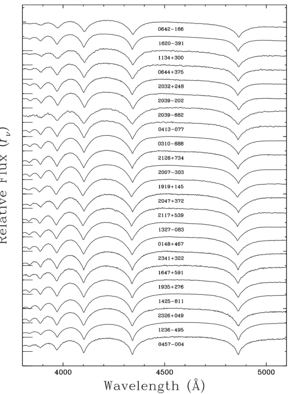
2.1 (a) Optical spectra of DA and DAZ white dwarfs . . . 57
2.1 (b) - continued. . . 58
2.1 (c) - continued. . . 59
2.2 Optical spectra of cool DA white dwarfs . . . 60
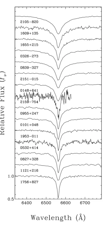
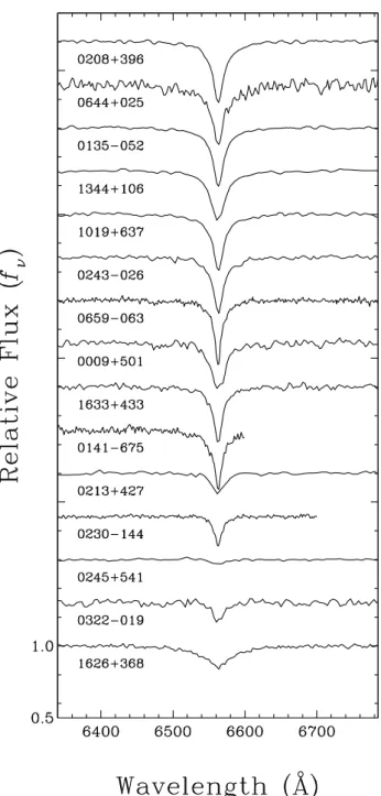
2.3 (a) Optical spectra of halpha from DA and DAZ white dwarfs . . . 61
2.3 (b) - continued. . . 62
2.3 (c) - continued. . . 63
2.3 (d) - continued. . . 64
2.4 (a) Optical spectra of DC White dwarfs . . . 65
2.4 (b) - continued. . . 66
2.4 (c) - continued. . . 67
2.5 (a) Optical spectra of DQ White dwarfs . . . 68
2.5 (b) - continued. . . 69
2.6 Optical spectra of DZ White dwarfs . . . 70
2.7 (V − I, V − K) two-color diagram . . . 71
2.8 MV vs. (V − I) color-magnitude diagram . . . 72
2.9 (a) Fits to the energy distributions . . . 73
2.9 (b) - continued. . . 74
2.9 (c) - continued. . . 75
2.9 (d) - continued. . . 76
2.9 (e) - continued. . . 77
2.9 (f) - continued. . . 78 2.9 (g) - continued. . . 79 2.9 (h) - continued. . . 80 2.9 (i) - continued. . . 81 2.9 (j) - continued. . . 82 2.9 (k) - continued. . . 83 2.9 (l) - continued. . . 84 2.9 (m) - continued. . . 85 2.9 (n) - continued. . . 86 2.9 (o) - continued. . . 87 2.9 (p) - continued. . . 88 2.9 (q) - continued. . . 89
2.10 (a) Fits to the energy distributions . . . 90
2.10 (b) - continued. . . 91
2.10 (c) - continued. . . 92
2.10 (d) - continued. . . 93
2.10 (e) - continued. . . 94
2.10 (f) - continued. . . 95
2.11 (a) Fits to the energy distributions of DQ stars . . . 96
2.11 (b) - continued. . . 97
2.11 (c) - continued. . . 98
2.12 (a) Fits to the energy distributions of DZ stars . . . 99
2.12 (b) - continued. . . 100
2.13 (a) - Fits to the optical spectra of the DA stars . . . 101
2.13 (b) - continued. . . 102
2.13 (c) - continued. . . 103
2.13 (d) - continued. . . 104
2.14 log g correction : fit through SDSS stars. . . 105
2.16 log g correction : spectroscopic vs. photometric masses. . . 107
2.17 Mass distribution vs. effective temperature. . . 108
2.18 Histogram of the ratio of helium- to hydrogen-rich WDs. . . 109
2.19 Mass distributions . . . 110
2.1 OBSERVATIONAL RESULTS . . . 40 2.1 continued. . . 41 2.1 continued. . . 42 2.1 continued. . . 43 2.1 continued. . . 44 2.1 continued. . . 45
2.2 RESULTS FROM PHOTOMETRIC FITS . . . 46
2.2 continued. . . 47
2.2 continued. . . 48
2.3 RESULTS FROM SPECTROSCOPIC FITS . . . 49
2.3 continued. . . 50
2.4 ADOPTED ATMOSPHERIC PARAMETERS OF NEARBY CANDIDATES . 51 2.4 continued. . . 52
2.4 continued. . . 53
2.4 continued. . . 54
2.4 continued. . . 55
Je tiens en premier lieu a remercier mon directeur de recherche Pierre Bergeron pour m’avoir accueillie dans son groupe et m’avoir fourni un sujet de recherche dans un domaine passionnant. J’aimerais ´egalement le remercier pour le temps et les efforts qu’il a fournis pour mon apprentissage et la r´ealisation de ma maˆıtrise.
Je tiens par la suite `a remercier ”les gars” du groupe : Alexandros, Patrick et Pier-Emmanuel (en ordre alphab´etique, bien sˆur!), pour avoir r´epondu `a toutes mes questions, pallier `a tous mes probl`emes dans ma recherche, pour l’aide constante `a la programmation en fortran, et pour les nombreuses sorties au pub et au Bar Lounge. Je ne peux aller plus loin sans remercier ma co-chambreuse Marie-Mich`ele, pour sa joie de vivre et son soutien moral quotidien, et surtout pour qui Saskatchewan et Espagne est toujours une bonne blague.
Un remerciement particulier `a Luc Turbide pour m’avoir sortie du p´etrin de nombreuses fois lors des diff´erentes r´ebellions de mon compte astro ou de mon ordinateur.
Un remerciement vraiment sp´ecial aux ”filles du bureau” : Am´elie (oui, tu y as une place honorifique), Cassandra, Marie-`Eve, Marilyn et Sandie. C’est un environnement de travail des plus agr´eables, dans lequel c’est un plaisir de travailler et de faire des pauses ”salon de th´e” aux heures les plus incongrues de la journ´ee (selon les voisins).
Je ne pourrais conclure ces remerciements sans parler du support exceptionnel de ma famille et belle-famille qui me soutient au quotidien (et lors de mes nuits au t´elescope!), et m’entoure chaleureusement. Merci `a Ben, V´ero (et Marilou), Louis- ´Etienne, Mikhail et Nadim pour toutes ces soir´ees endiabl´ees qui m’ont permis de bien d´ecompresser. Antoine, merci de m’avoir appris que ”seule une personne m´ediocre peut atteindre le summum de ses capacit´es”, et que ”brebis enrag´ee est pire que loup”, avec ¸ca je ne peux que r´eussir dans la vie.
Introduction
Les naines blanches repr´esentent le dernier stade ´evolutif de pr`es de 97 % des ´etoiles de la s´equence principale, incluant notre Soleil. En effet, une naine blanche r´esulte de l’effondrement gravitationnel du cœur d’une ´etoile g´eante rouge. Ce cœur restant, d´eg´en´er´e, qui a ´epuis´e son carburant nucl´eaire, se refroidit inexorablement pendant des milliards d’ann´ees. Leur faible brillance et le fait que celle-ci ne cesse de diminuer, rendent les naines blanches des cibles tr`es difficilement d´etectables du point de vue observationnel. Le fait mˆeme de leur existence n’a ´et´e d´ecouvert qu’au milieu du XIXesi`ecle, et il a fallu attendre le d´ebut du XXesi`ecle pour pouvoir d´ecrire th´eoriquement ces objets `a l’aide, en grande partie, des nouveaux d´eveloppements dans le domaine de la m´ecanique quantique.
Malgr´e cela, il est d’un int´erˆet majeur de comprendre dans ses moindres d´etails la popu-lation de naines blanches car ces ´etoiles forment une classe unique de la population stellaire globale, et sont de ce fait un marqueur important de l’´evolution de la Galaxie. La distribu-tion de masse, la densit´e spatiale et la composition chimique, entre autres, sont des indices importants permettant de mieux retracer et contraindre ces chemins ´evolutifs. La fonction de luminosit´e des naines blanches, qui est une mesure de la densit´e spatiale en fonction de la luminosit´e intrins`eque, est un outil des plus pr´ecieux pour estimer l’ˆage du disque Galactique. Mais afin de pouvoir extraire des informations pertinentes de ces diagnostics, l’´echantillon d’´etoiles utilis´e se doit d’ˆetre le plus complet possible pour ˆetre statistiquement viable.
lumi-nosit´e qui sont difficiles `a ´etudier d`es que l’on s’´eloigne un tant soit peu du Soleil. Il n’existe pas de grands relev´es exclusifs aux naines blanches, `a proprement parler. La d´etection de naines blanches est souvent r´ealis´ee par le biais de relev´es limit´es par la magnitude ou par le mouvement propre. Les relev´es caract´eris´es par les grands mouvements propres, tels que les relev´es du NLTT (New Luyten Two-Tenths), du LSPM (L´epine-Shara Promper Motion) et du SuperCOSMOS-RECONS (Research Consortium on Nearby Stars), se basent sur le d´eplacement relatif de certaines ´etoiles par rapport aux ´etoiles distantes (et immobiles en apparence), `a deux ´epoques distinctes. En couplant ces mouvements propres `a des indices de couleur, on peut ainsi distinguer les naines blanches d’autres populations stellaires. Malgr´e le fait que cette technique soit couramment utilis´ee dans un grand nombre de relev´es, il reste que les inconv´enients sont majeurs. Les relev´es `a grand mouvement propre sont grandement biais´es par la cin´ematique des ´etoiles. De plus, les r´egions dens´ement peupl´ees, tel que le plan galactique, sont g´en´eralement ´evit´ees, dˆu aux limites de la m´ethode de d´etection.
Des contributions majeures sur la connaissance actuelle de la population des naines blanches ont ´et´e ´egalement r´ealis´ees `a l’aide de relev´es mesurant l’exc`es de rayonnement ultraviolet (UV), une technique majoritairement employ´ee parmi les relev´es photom´etriques permettant l’identification de candidates naines blanches chaudes. Les ´etudes bas´ees sur les relev´es `a exc`es dans l’UV permettent de construire la partie chaude de la fonction luminosit´e, comme celles r´ecemment d´etermin´ees `a partir des relev´es Palomar Green (PG; Liebert et al. 2005) et Kiso (Limoges & Bergeron 2010). L’identification de candidates naines blanches par l’exc`es d’UV comporte par contre des restrictions importantes, en ne ciblant uniquement que les objets les plus bleus, et par le fait mˆeme des objets chauds. Il est difficile de g´en´erer un ´echantillon complet `a l’aide de cette m´ethode, et il ne nous est pas permis d’obtenir de l’information sur la partie froide de la fonction luminosit´e.
Les relev´es bas´es sur le mouvement propre et la colorim´etrie mentionn´es pr´ec´edemment ne s’entrecoupent pas, et sont par le fait mˆeme incomplets. La seule possibilit´e d’obtenir un ´echantillon statistiquement repr´esentatif est d’utiliser un ´echantillon complet limit´e par le volume, centr´e autour du Soleil. Un tel ´echantillon permet d’obtenir un mod`ele statistique-ment pr´ecis tant que le compromis entre la compl´etude et la taille de l’´echantillon est bien
respect´e. On veut principalement ´eviter de se retrouver avec un ´echantillon enti`erement connu mais ayant un nombre trop limit´e d’´etoiles. Avec un ´echantillon complet, il est ainsi possible d’extrapoler notre connaissance de la population locale `a celle des naines blanches dans leur ensemble, tels que la densit´e de masse ou la densit´e spatiale des naines blanches dans le disque galactique, ou mˆeme dans le halo.
De nombreuses ´etudes ayant pour cible la compl´etude et la caract´erisation de l’´echantillon de naines blanches dans le voisinage solaire ont ´et´e r´ealis´ees. La premi`ere ´etude enti`erement d´edi´ee `a la d´efinition d’un relev´e complet de naines blanches proches a ´et´e r´ealis´e par Holberg et al. (2002). La limite de distance de 20 pc a ´et´e choisie pour correspondre au volume d´efini par le relev´e de NSTARS, une banque de donn´ees regroupant l’information disponible sur tous les objets pr´esents aux alentours du Soleil. En se basant sur l’´etude de Holberg et al. (2002), le volume d´efini par la limite arbitraire de 20 pc semble raisonnable en ce qui a trait `a la compl´etude. La d´etermination de candidates probables est enti`erement bas´ee sur les magni-tudes photom´etriques tir´ees du Villanova White Dwarf Catalog. Deux crit`eres de s´election ont ´et´e utilis´es afin de d´eterminer les naines blanches confin´ees `a l’int´erieur d’un volume de 20 pc de rayon. La priorit´e a ´et´e donn´ee aux objets ayant une parallaxe trigonom´etrique π≥ 0.”05, les pla¸cant ainsi directement `a l’int´erieur de la limite voulue. Pour les ´etoiles n’ayant pas de parallaxes disponibles, le deuxi`eme crit`ere de s´election employ´e utilise des estim´es de distance photom´etrique bas´e sur le calcul de V − MV ≤ 1.505. Une attention particuli`ere a ´et´e port´ee sur la d´etection d’anomalies notoires parmi les ´etoiles s´electionn´ees, qui ont ´et´e retir´ees de l’´echantillon. Comme Holberg et al. (2002) le mentionne, la qualit´e des donn´ees ainsi retrac´ees est loin d’ˆetre uniforme, et pr´esente surtout de grandes inhomog´en´eit´es. Afin d’ˆetre plus sou-cieux de la qualit´e des donn´ees, un ordre hi´erarchique a ´et´e adopt´e, en priorisant les indices de couleurs Johnson B − V , Str¨omgren b − y et multichannel g − r, autant que possible. L’effet direct de cette s´election m`ene `a de grandes inhomog´en´eit´es dans le calcul des magni-tudes absolues et, par propagation, sur l’estimation des distances. L’analyse r´ealis´ee avec cet ´echantillon nouvellement d´etermin´e ´etait enti`erement concentr´ee sur le calcul de la densit´e spatiale locale et sur l’estimation de la compl´etude de cet ´echantillon. En se basant sur l’hy-poth`ese d’un ´echantillon `a 13 pc connu dans son int´egralit´e, Holberg et al. (2002) estime alors
que l’´echantillon local est complet `a 65%. Mis `a part les diff´erents types spectraux, aucuns d´etails concernant les param`etres atmosph´eriques des naines blanches dans le voisinage solaire ne sont pr´esent´es.
La recherche de naines blanches dans l’´echantillon local de 109 candidates tir´e de Holberg et al. (2002) s’est poursuivie par le travail de Vennes & Kawka (2003), Kawka et al. (2004) et Kawka & Vennes (2006), en utilisant le catalogue NLTT r´evis´e de Salim & Gould (2003), un relev´e bas´e sur le mouvement propre des ´etoiles. En combinant des diagrammes couleur-couleur `
a des diagrammes de mouvement propre r´eduit, ainsi qu’en effectuant un suivi spectroscopique des candidates naines blanches, il a ´et´e possible de faire une mise `a jour de l’´echantillon local de Holberg et al. (2002), plusieurs ´etoiles ayant ´et´e rajout´ees et d’autres retir´ees de l’´echantillon. Mentionnons, en particulier, la contribution importante de Kawka & Vennes (2006) `a cette recherche, en identifiant spectroscopiquement 8 naines blanches se situant `a moins de 20 pc du Soleil. Farihi et al. (2005), Subasavage et al. (2007) et Subasavage et al. (2008) ont ´egalement contribu´e `a l’augmentation de l’´echantillon local connu avec les d´ecouvertes de quelques autres candidates.
Holberg et al. (2008) et Sion et al. (2009) ont par la suite repris l’´etude des naines blanches dans le voisinage solaire de Holberg et al. (2002) en rassemblant les d´ecouvertes r´ecentes men-tionn´ees ci-dessus, pour former un nouvel ´echantillon de 132 ´etoiles. Ce faisant, les candidates locales ayant de nouveaux estim´es de distance `a plus de 20 pc ont ´et´e ´elimin´ees de l’´echantillon. Les param`etres atmosph´eriques des naines blanches de l’´echantillon local ont ´et´e compil´es par Holberg et al. (2008) `a partir de nombreuses sources diff´erentes. `A l’aide de ces donn´ees, la masse moyenne de l’´echantillon ainsi qu’une nouvelle estimation de la densit´e spatiale ont pu ˆetre calcul´ees en utilisant une vari´et´e d’estimations de distance, combinant parallaxes tri-gonom´etriques, analyses spectroscopiques et photom´etriques. De son cˆot´e, l’´etude de Sion et al. (2009) est enti`erement ax´ee sur les propri´et´es cin´ematiques ainsi que la distribution des diff´erents types spectraux des naines blanches `a moins de 20 pc du Soleil.
Ce manque de coh´erence entre les diff´erents mod`eles d’atmosph`ere et les techniques d’ana-lyse repr´esente le talon d’Achille des ´etudes de l’´echantillon local r´ealis´ees jusqu’`a pr´esent. Les analyses qui en ont d´ecoul´e sont donc teint´ees d’incertitudes, et les propri´et´es de l’´echantillon
local qui en ont ´eman´e sont peu fiables. La quˆete d’un ´echantillon complet de naines blanches dans le voisinage solaire est encore une pr´eoccupation actuelle (voir les travaux de Limoges et al. 2010, entres autres), alors que jusqu’`a aujourd’hui, toute analyse compl`ete `a partir d’un mˆeme ensemble de donn´ees fut laiss´ee de cˆot´e. Il est donc tout `a fait appropri´e de reconsid´erer la population locale d’´etoiles naines blanches en proc´edant `a une analyse rigoureuse, r´ealis´ee de mani`ere homog`ene, de chaque ´etoile de cet ´echantillon.
Le chapitre 3 pr´esente, sous la forme d’une publication qui sera ´eventuellement soumise `
a l’Astrophysical Journal, l’int´egralit´e de l’´etude r´ealis´ee sur l’´echantillon des naines blanches dans le voisinage solaire. On pr´esente dans un premier temps la s´election de l’´echantillon local ainsi que les donn´ees spectroscopiques et photom´etriques utilis´ees, suivi d’une description d´etaill´ee des mod`eles d’atmosph`ere et des techniques d’analyse employ´ees dans notre ´etude. L’analyse globale r´ealis´ee `a partir des param`etres atmosph´eriques nouvellement d´etermin´es est ensuite expos´ee, incluant une ´etude de la distribution de la composition chimique, de la distribution de masse et de la fonction luminosit´e des naines blanches dans le voisinage solaire.
Know Your Neighborhood: A
Detailed Model Atmosphere
Analysis of Nearby White Dwarfs
N. Giammichele1, P. Bergeron1, & P. Dufour1
To be submitted to The Astrophysical Journal December 2010
1. D´epartement de Physique, Universit´e de Montr´eal, C.P. 6128, Succ. Centre-Ville, Montr´eal, Qu´ebec H3C 3J7, Canada.
2.1
Abstract
We present improved atmospheric parameters of nearby white dwarfs lying within 20 pc of the Sun. The aim of the current study is to obtain the best statistical model of the least-biased sample of the white dwarf population. A homogeneous analysis of the local population is performed combining detailed spectroscopic and photometric analyses based on improved model atmosphere calculations for various spectral types including DA, DB, DQ, and DZ stars. The spectroscopic technique is applied to all stars in our sample for which optical spectra are available. Photometric energy distributions, when available, are also combined to trigonometric parallax measurements to derive effective temperatures, stellar radii, as well as atmospheric compositions. A revised catalog of white dwarfs in the solar neighborhood is presented. We provide for the first time a comprehensive analysis of the mass distribution and the chemical distribution of white dwarf stars in a volume-limited sample.
2.2
Introduction
It is of major interest to fully understand the white dwarf population as it is a significant part of the global stellar population and a major indicator of the evolutionary history of the Galaxy. Mass distribution, space density, and chemical composition are most valuable pieces of information to better constrain their evolutionnary history. The luminosity function of the white dwarf population, defined as the number of white dwarfs as a function of their intrinsic luminosity, can be a precious tool to narrow down the age of the Galactic disk. But in order to take the greatest advantage of these indications, the white dwarf population sampled must be as close as possible to a statistical completion.
The white dwarf population is composed mainly of low-luminosity stars that are rather difficult to study as we get further away from the Sun. Candidates are mainly discovered from either proper-motion-limited or magnitude-limited surveys. Proper-motion surveys are characterized by the finding of high-proper motion stars through a comparison of identical fields observed at two different epochs. By further combining these proper motions with color indices, white dwarfs can be successfully distinguished from other objects. Despite its wide use
in the building of major surveys, important flaws remain. Proper-motion surveys naturally present a high kinematic bias. Moreover, high density regions, such as the galactic plane, are usually avoided.
Major contributions to the knowledge of the white dwarf population were made through ultraviolet excess surveys, a technique primarily used among photometric surveys to identify hot white dwarf candidates. Studies based on ultraviolet excess surveys lead to the building of the bright end of luminosity function, like those recently derived from the Palomar Green (PG; Liebert et al. 2005) and the Kiso surveys (Limoges & Bergeron 2010). However, the restriction to the detection of only bluer and thus hotter objects represents a major bias in the case of ultraviolet excess surveys. Therefore, building a complete sample is highly compromised and does not allow us to obtain essential information on the faint end of the luminosity function. Proper-motion-limited and magnitude-limited surveys are not cross-correlated and are both incomplete. The one possibility to get a less biased sample is to use a complete volume-limited sample, centered around the Sun. Such a sample can provide an accurate statistical model as long as the right balance of high completeness and small number statistics is achieved. A precise picture of the local sample can reliably be extended to the rest of the Galaxy to get important details on the white dwarf population, such as the mass density and the space density of white dwarfs within the galactic disk.
Numerous studies were performed aiming to complete and to characterize the sample of nearby white dwarfs. The first study dedicated to building a complete census of the local sample of white dwarfs was performed by Holberg et al. (2002). The distance of 20 pc was chosen to correspond to the volume of the NSTARS database, a program aimed at compiling information on possibly all stellar sources near the Sun, and at better understanding the local stellar population. As Holberg et al. (2002) further discussed in their work, the volume then defined by the 20 pc limit was assumed to be reasonably complete. The determination of the possible candidates was entirely based on photometric magnitudes collected from the Villa-nova White Dwarf Catalog. Two main selection criteria were used to determine white dwarfs within 20 pc. First, the WD catalog was searched for objects with trigonometric parallaxes
de-termined distances based on V − MV ≤ 1.505. Careful attention was paid to remove manually obvious known anomalies. As Holberg et al. (2002) reported, data retrieved in this manner were far from uniform in quality and not homogeneous in any way. A priority scheme was adopted to cope with the different data sources, giving a higher priority to Johnson B− V , Str¨omgren b− y, and multichannel g − r color indices, when possible. The direct effect of this selection led to major inhomogeneities in the calculations of absolute visual magnitudes and resulting distances. The analysis made afterwards based on this local sample was uniquely drawn towards the calculation of the local space density and the estimation of the complete-ness of the sample. Based on the assumption that the 13 pc sample is entirely known, Holberg et al. (2002) estimated the 20 pc sample to be 65% complete. Few details showing the at-mospheric properties of the white dwarfs in the solar neighborhood were presented at that time.
The quest for completeness of the local sample of white dwarfs based on the 109 candidates determined by Holberg et al. (2002) was pursued by the contributions of Vennes & Kawka (2003), Kawka et al. (2004), and Kawka & Vennes (2006) who surveyed the revised NLTT catalog of Salim & Gould (2003). By using color-color and reduced proper motion diagrams, as well as a spectroscopic follow-up of white dwarf candidates, several stars were added to the original local sample, while some others were removed. In particular, Kawka & Vennes (2006) extended the search for possible candidates by spectroscopically identifying 8 new white dwarfs lying within 20 pc. Other contributions from Farihi et al. (2005), Subasavage et al. (2007), and Subasavage et al. (2008) are also worth mentioning in the finding of new local candidates.
Holberg et al. (2008) and Sion et al. (2009) reanalyzed the white dwarfs in the solar neighborhood by updating the local sample of Holberg et al. (2002) with the recent discoveries mentioned above, to form a sample composed of 132 stars. Holberg et al. (2008) gathered atmospheric parameters of the local sample candidates, collected from numerous sources, to calculate the mean mass of the sample, and used a variety of spectroscopic, photometric, and trigonometric distances to better estimate the local space density. Sion et al. (2009) strictly focused on the kinematical properties and the distribution of spectroscopic subtypes of the
white dwarf population within 20 pc.
The lack of consistency from the different model atmospheres and methods used makes previous analyses of the ensemble properties of the local white dwarf sample quite uncertain, and may lead to erroneous estimates. Obviously, the quest for the local sample completeness is still a central preoccupation, while proper analysis of such a sample has been left aside, as up to now, there is no detailed study regrouping all available data. Given these restrictions, it is appropriate to revisit the nearby white dwarf population by performing a rigorous analysis, in an homogeneous fashion, of every star in the sample.
In this paper, we present improved atmospheric parameters of all possible nearby white dwarfs lying within 20 pc of the Sun. A homogeneous and complete analysis of the local population is performed combining detailed spectroscopic and photometric analyses based on improved model atmosphere calculations for various spectral types including DA, DC, DQ, and DZ stars. Our photometric and spectroscopic observations are presented in Section 2.4, while the theoretical framework and fitting techniques are exposed in Section 2.5. The global properties of our sample, including the mass distribution and luminosity function are examined in Section 2.6. Our conclusions follow in Section 2.7.
2.3
Definition of the Local Sample
Our sample is composed of spectroscopically identified white dwarfs that lie in the solar neighborhood, within the approximate 20 pc defined limit. It is mostly drawn from the com-plete list presented in Sion et al. (2009), an updated version of the local population defined by Holberg et al. (2002, 2008). As mentioned earlier, significant additions to this initial sample have been made by Kawka et al. (2004), Kawka & Vennes (2006), and Subasavage et al. (2007, 2008), with some contributions from other studies (see references in Sion et al. 2009). We increased the sample size by taking into account all possible white dwarfs that could lie within the error limit inside the 20 pc region, which means including all objects presented in Table 5 of Holberg et al. (2008). We include here the peculiar DQ star LHS 2229 (1008+290) since a new trigonometric parallax made available to us by H. C. Harris. (2010, private com-munication) places the star inside the 20 pc region. Also, we include the DC star LHS 1247
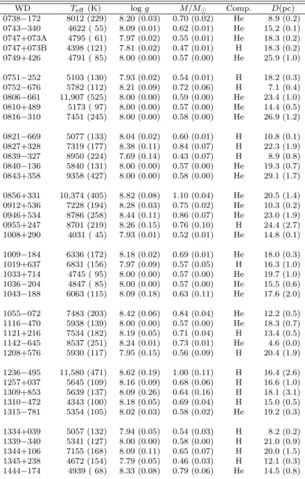
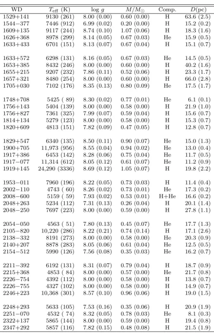
(0123−262) since its distance, estimated from the photometric observations of Bergeron, Ruiz, & Leggett (1997, hereafter BRL97), places this candidate inside our region of interest, within the uncertainties. Finally, an initial sample of 167 white dwarf stars has been retained for this analysis. The complete list of objects is presented in Table 2.1 where we give for each star the WD number from the Villanova White Dwarf Catalog as well as an alternate name; whenever possible we used the LHS or the Giclas names unless the object is better known under another name in the literature. The additional entries for each object are described in the next section.
2.4
Observations
2.4.1 Spectroscopic Observations
One of the original goals of this project was to characterize the best we could the white dwarf population in the solar neighborhood, which implies at first to provide a spectroscopic snapshot of this population in the form of an atlas similar to that published by Wesemael et al. (1993). Spectroscopic observations at high signal-to-noise ratio were thus secured for 136 objects in our sample. Most of the blue spectra (λ ∼ 3700 − 5200 ˚A) for the DA white dwarfs were already available to us from of our numerous studies of these stars (see, e.g., Liebert et al. 2005), while several spectra covering the region near Hα, required to constrain the atmospheric composition of the coolest degenerates, were taken from the studies of BRL97 and Bergeron, Leggett, & Ruiz (2001, hereafter BLR01).
New optical spectra for 23 objects in our sample were acquired for the specific purpose of this project during several observing runs at the Steward Observatory 2.3 m telescope equipped with the Boller & Chivens spectrograph and a Loral CCD detector. The 4.”5 slit together with the 600 l mm−1 grating in first order provided a spectral coverage from about 3200 to 5300 ˚A at an intermediate resolution of ∼ 6 ˚A FWHM. Spectra were also obtained with the Kitt Peak National Observatory 2.1 m and 4 m telescopes equipped with the RC and Goldcam spectrographs, respectively. Both used a 2.”0 slit with a resolution of ∼ 6 ˚A FWHM, but different gratings of 316 l mm−1 and 500 l mm−1, respectively. Further details
on the observing and reduction procedure can be found in Saffer et al. (1994).
The spectral types of each white dwarf in our nearby sample are reported in Table 2.1. Otherwise noted in the last column, all spectral types have been confirmed from our own spectroscopic observations. In summary, this sample breaks down into the following spectral types: 111 DA, 26 DC, 19 DQ, 10 DZ and 1 DBQA. Strangely enough, there is not a single warm (Teff > 13, 000 K) DB star in this nearby sample. According to our ongoing spectroscopic
analysis of relatively bright DB stars (Bergeron et al. 2010), the closest DB stars lies at∼ 30 pc.
Figure 2.1(a-c) presents the DA and DAZ spectra in our sample in order of decreasing effective temperatures (determined below using the spectroscopic technique, see Section 2.5.4). The DAZ stars are easily recognized by the presence of the Ca ii H and K lines, the most notable DAZ star in this sample being GD 362 (1729+371) whose spectrum also shows spectral lines from Ca i, Mg i, and Fe i (Gianninas et al. 2004). The spectrum of LHS 1660 (0419−487) is also contaminated by the presence of an M dwarf companion. GR 431 (0939+071), also known as PG 0939+072, is a problematic object. Classified DC7 in the PG catalog, it was not included in the spectroscopic analysis of DA white dwarfs in the PG survey of Liebert et al. (2005), despite the fact that it had been reclassified as DA2 in Holberg et al. (2002). However, it appeared again as DC7 in Table 4 of Holberg et al. (2008), a list of possible white dwarfs within 20 pc. Our spectrum, presented in Figure 2.1(c), shows that GR 431 is not a white dwarf. Our spectroscopic fit for this star yields Teff ∼ 6800 K and log g = 6.9, too low
for a white dwarf; this star is therefore excluded from our analysis.
The blue spectra for the DA and DAZ stars too cool to be analyzed using line profile fitting techniques are displayed in Figure 2.2. In some cases, these objects are completely featureless in the spectral region shown here, which implies that only Hα can be detected spectroscopically.
The DA stars in our sample for which spectra at Hα are also available are presented in Figure 2.3(a-d) as a function of decreasing equivalent widths. The Zeeman triplet in the magnetic white dwarf LHS 1734 (0503−174) is clearly visible. The presence of Hα in the coolest white dwarfs is crucial to better constrain the atmospheric parameters using the photometric
method described in Section 2.5.2. The coolest DA stars in which Hα can be detected in our sample have photometric temperatures around Teff ∼ 5000 K.
Our set of DC white dwarfs, with featureless spectra, as well as the spectrum for LDS 678A (1917−077), the only DBQA star, are displayed in Figure 2.4(a) in order of right ascension. For clarity the spectra have been normalized to a continuum set to unity. Subsets of DC stars with only blue and red spectral coverage are also displayed in Figure 2.4(b-c). Spectroscopic data of some DQ stars in our sample are displayed in Figure 2.5(a). Because of the spectral classification scheme devised by McCook & Sion (1999), DQ white dwarfs may have carbon features detectable only in the ultraviolet, hence some spectra shown here appear featureless in the optical; note the presence of the CH band in the spectrum of G99-37 (0548−001), one of the only two such stars known. Additional DQ stars are shown in Figure 2.5(b). At the top of the figure is shown a normal DQ stars with very strong C2 Swan bands. Note how these
molecular bands in the other objects shown in this figure appear shifted and more symmetrical with respect to this normal DQ star, with the extreme case of LHS 2229 (1008+290) displayed at the bottom. This phenomenon has recently been explained by Kowalski (2010) as a result of pressure shifts of the carbon bands that occurs in cooler, helium-dominated atmospheres. The presence of a very strong magnetic field has also been reported in the bottom two objects (see, e.g., Schmidt et al. 1999). These stars are now being classified as DQpec.
Finally, our DZ spectra, showing the presence of metal lines, mainly the Ca ii H & K doublet, are displayed in Figure 2.6. Both L745-46A (0738−172) and Ross 640 (1626+368) are actually DZA stars with very shallow Hα absorption lines (shown in Fig. 2.3), resulting from the presence of a trace of hydrogen in a helium-dominated atmosphere.
It is interesting to note that the local population of white dwarfs includes some of the strangest stars we know, including those mentioned above which are unique objects, but also GW+70 8247 (1900+705), a heavily magnetic white dwarf; G47-18 (0856+331), a unique DQ star that shows both C2 Swan bands and C i atomic lines; BPM 27606 (2154−512), one
of the DQ stars with the strongest C2 Swan bands; G240-72 (1748+708) whose spectrum
is characterized by a deep yellow sag in the 4400-6300 ˚A region (see Fig. 2.5(a) and also Wesemael et al. 1993); LP 701-29 (2251−070), a heavily blanketed DZ star, the only known
case where Ca i λ4226 appears stronger than the Ca II doublet. Definitely, we live in strange neighborhood.
2.4.2 Photometric Observations
Optical BV RI and infrared J HK photometric data were retrieved for 82 cool white dwarfs in our sample, taken mainly from the detailed studies of BRL97 and BLR01. Complete details of the observing procedure and data reduction are provided in these references. For 26 addi-tional cool degenerates remaining with no available data, optical V magnitudes were obtained from different sources, mainly from the online version of the Villanova White Dwarf Catalog, while infrared J HKS photometry was extracted from the online version of the Two Micron All Sky Survey (2MASS) survey. The optical and infrared photometric data are reported in Table 2.1; references for the adopted photometry are provided in the last column. Typical photometric uncertainties are 3% at V , R, and I, and 5% elsewhere (BLR01). Uncertainties for the V magnitudes retrieved from the White Dwarf Catalog vary widely and we simply assume 5% for simplicity.
The (V − I, V − K) two-color diagram is displayed in Figure 2.7 for 71 white dwarfs in our sample. DA and non-DA stars are represented by filled and open circles, respectively. Also shown are the predictions from pure hydrogen and pure helium cooling sequences at log g = 8.0 using the photometric calibration of Holberg & Bergeron (2006). DA and non-DA stars form two distinct narrow sequences in this diagram, which follow closely the behavior of the model sequences. Worth mentioning here is a complete absence of non-DA stars in a particular range of V−K colors between ∼1.2 and 1.7, which corresponds to the so-called non-DA gap first discussed by BRL97. There are also several outliers in this diagram, identified in the figure, all of the non-DA type: BPM 27606 (2154−512) is a DQ star with very strong C2 Swan bands (see Figure 2.5) that affect the V magnitude; LHS 1126 (0038−226) shows a
strong infrared flux deficiency which has been interpreted by Bergeron et al. (1994) in terms of the H2-He collision-induced absorptions in a mixed H/He atmosphere; ER 8 (1310−472)
is the coolest and oldest white dwarf identified in the analysis of BRL97, and it has a pure hydrogen atmospheric composition despite its non-DA nature; G195-19 (0912+536) is a∼ 100
MG magnetic white dwarf with some unidentified spectroscopic features (Schmidt & Smith 1994) that affect the I magnitude.
Data sets appropriate for a photometric or spectroscopic analysis could not be found for 3 remaining stars (0208−510, 0415−594, and 1132−325), the first two of which are Sirius-like systems. These objects had to be left aside in the present analysis.
2.4.3 Trigonometric Parallax Measurements
BRL97 found that even though the model energy distributions are somewhat sensitive to surface gravity, it is practically impossible to determine log g from the observed photometry alone. Only for stars with available trigonometric parallax measurements is it possible to determine the stellar radius, and thus the mass through the mass-radius relation. In our sample, 109 stars have trigonometric parallax measurements taken from the Yale parallax catalog (van Altena et al. 1994, hereafter YPC) and the Hipparcos parallax catalog (Perryman & ESA 1997), with the exception of LHS 1044 (0011−134; Bergeron et al. 1992b), vB 3 (0743−340; Ruiz et al. 1989), — LHS 1243, SCR 0753−2524, SCR 0821−6703, LEHPM 2− 220, L104−2, L40−116 and SCR 2012−5956 (0121−429, 0751−252, 0821−669, 1009−184,
1223−659, 1315−781 and 2008−600; Subasavage et al. 2009)— , GD 362 (1729+371; Kilic et
al. 2008), LEHPM 4466 (2211-392; Ducourant et al. 2007), and LHS 2229 (1008+290; H. C. Harris, private communication); these values and corresponding uncertainties are reported in Table 2.1.
The MV versus (V − I) color-magnitude diagram obtained using these trigonometric pa-rallaxes is displayed in Figure 2.8 for 74 stars in our sample, with available V and I colors. Again, white dwarfs are distinguished in terms of their DA or non-DA spectral types, and the predictions from pure hydrogen and pure helium cooling sequences at log g = 8.0 are superimposed on the observed data.
As mentioned by BLR01, DA and non-DA stars form well-defined narrow sequences in this diagram, although not as narrow as those observed in the previous figure, most likely because the trigonometric parallax measurements come from inhomogeneous parallax samples. In general, non-DA stars appear less luminous than DA stars, a result that can be explained
if non-DA stars are more massive, and thus possess smaller radii, than their DA counterpart. Also, all overluminous white dwarfs are of the DA spectral type. As discussed in BRL97, most, if not all, of these objects are unresolved binaries — e.g., L870-2 (0135−052) — and their luminosity is the contribution of two white dwarfs with probably normal masses.
2.5
Atmospheric parameter determinations
2.5.1 Theoretical Framework
Our synthetic spectra are built from the new LTE model atmosphere code described at length in Tremblay & Bergeron (2009) and references therein, which uses improved calcu-lations for the Stark broadening of the hydrogen line profiles. The theoretical spectra are calculated within the occupation formalism of Hummer & Mihalas (1988), with the inclusion of nonideal perturbations from protons and electrons directly inside the unified theory of Stark broadening of Vidal et al. (1970). Models take into account convective energy transport and hydrogen molecular opacity up to an effective temperature at which non-local thermodynamic equilibrium (NLTE) effects are still negligible and the atmospheres are completely radiative (Teff = 40, 000 K). Above this temperature, the TLUSTY and SYNSPEC packages are used
to deal with NLTE effects present in hotter stars. The resulting homogeneous model grid thus consistently includes NLTE effects, as well as convective energy transport following the revised ML2/α = 0.8 prescription of the mixing-length theory (see Bergeron et al. 1995 and Tremblay & Bergeron 2009 for details). For helium-dominated stars, model atmospheres and synthetic spectra include the improved Stark profiles of neutral helium of Beauchamp et al. (1997). Additional models for DQ and DZ stars are described below.
Our model grid covers a range of effective temperature between Teff = 1500 K and 45,000 K
by steps of 500 K for Teff < 15, 000 K, 1000 K up to Teff = 18, 000 K, 2000 K up to Teff = 30, 000
K, and by steps of 5000 K above. The log g ranges from 6.5 to 9.5 by steps of 0.5 dex, with additional models at log g = 7.75 and 8.25. Additional models, in particular for cool stars, have been calculated with mixed hydrogen and helium compositions of log (H/He) =−1.0 to 3.0 (in steps of 0.5).
2.5.2 Photometric Technique
Atmospheric parameters, Teff and log g, and chemical compositions of cool white dwarfs can
be measured accurately using the photometric technique developed by BRL97. We first convert optical BV RI and infrared J HK (or J HKS from 2MASS) photometric measurements into observed fluxes and compare the resulting energy distributions with those predicted from our model atmosphere calculations. To accomplish this task, we first transform every magnitude
m into an average flux fλm using the equation
m =−2.5 log fλm+ cm , (2.1) where fλm= ∫∞ 0 fλSm(λ)λ dλ ∫∞ 0 Sm(λ)λ dλ , (2.2)
and where Sm(λ) is the transmission function of the corresponding bandpass, fλ is the mo-nochromatic flux from the star received at Earth, and cm is a constant to be determined. The transmission functions are taken from Landolt (1992a,b) for the BV RI filters on the Johnson-Kron-Cousins CTIO photometric system, and from Bessell & Brett (1988) for the
J HK filters on the Johnson-Glass system. Infrared magnitudes on the CIT system taken
from BRL97 and BLR01 first need to be transformed on the Johnson-Glass system using the equations given by Leggett (1992). For J HKS, we used the transmission functions from the 2MASS set defined by Cohen et al. (2003).
The constants cm for each passband are determined using the improved calibration fluxes from Holberg & Bergeron (2006), defined with the Hubble Space Telescope (HST) absolute flux scale of Vega. The calculations yield cB =−20.45645, cV =−21.06067, cR=−21.64393,
cI =−22.38477, cJ =−23.75551, cH =−24.84898, and cK =−25.99941. For the 2MASS set,
we find instead cJ =−23.76771, cH =−24.86404, and cKS =−25.92455.
For each star in Table 2.1, a minimum set of four average fluxes fλm is obtained that can be compared with model fluxes. Since the observed fluxes correspond to averages over given bandpasses, the monochromatic fluxes from the model atmospheres need to be converted
into average fluxes as well, Hm
λ , by substituting fλ in equation 2.2 for the monochromatic Eddington flux Hλ. We can then relate the average observed fluxes fλm and the average model fluxes Hλm — which depend on Teff, log g, and He/H — by the equation
fλm= 4π(R/D)2Hλm (2.3)
where R/D defines the ratio of the radius of the star to its distance from Earth. We then minimize the χ2 value defined in terms of the difference between observed and model fluxes
over all bandpasses, properly weighted by the photometric uncertainties. Our minimization procedure relies on the nonlinear least-squares method of Levenberg-Marquardt (Press et al. 1986), which is based on a steepest decent method. Only Teff and the solid angle π(R/D)2 are
considered free parameters, and the uncertainties of both parameters are obtained directly from the covariance matrix of the fit. For white dwarfs with no parallax measurement, we simply assume a value of log g = 8.0.
Our results for the analysis of optical and J HK photometric data sets are presented in Figure 2.9(a-q), and in Figure 2.10(a-f) for the 2MASS J HKSdata sets. Observed fluxes in the left panels are represented by error bars, while model fluxes are shown as open or filled circles depending on the atmospheric composition. The atmospheric parameters of each solution are indicated in the panel. On the right panels are shown the spectroscopic observations near Hα compared to the model atmosphere predictions assuming the pure hydrogen solution; these only serve as an internal check of our photometric solutions and are not used in the fitting procedure. For instance, cases where an Hα absorption feature is predicted but is not observed clearly suggest that the pure helium solution is more appropriate. In cases where the star is too cool to show Hα (Teff . 5000 K), however, one has to rely on the predicted energy
distributions to decide which atmospheric composition best fit the photometric data. Based on our inspection of these fits, we adopt the solutions shown in red in the left panels.
In general, the fits to the energy distributions, and the internal consistency with the ab-sence or preab-sence of Hα, are excellent. Several objects in Figure 2.9 are worth discussing, however. LHS 1008 (0000−345) belongs to this strange class of objects reported by BRL97 whose energy distributions are better fit with pure hydrogen models, yet their spectra are
fea-tureless near the Hα region. There are three weakly magnetic white dwarfs shown here — LHS 1044 (0011−134), LHS 1734 (0503−174), and G99-47 (0553+053), all three of which exhibit the Zeeman triplet; the predicted Hα profiles shown here do not include the magnetic field. For LHS 1126 (0038−226), a mixed abundance of He/H ∼ 100 was required to reproduce the infrared flux deficiency, as discussed above. Some of the strongest DZ stars, vMa 2 (0046+051) for instance, show a small disagreement for the B bandpass where the Ca ii H & K doublet depresses the observed flux significantly. Such DZ stars will be analyzed in greater detail in the next section. Some DA stars — L587-77A (0326−273) and L532-81 (0839−327) — show a strong discrepancy between the observed and predicted profiles; since they are also low surface gravity objects, these are most likely unresolved double degenerate systems composed of two DA stars. Note that the absorption feature seen in G47-18 (0856+331) is a neutral carbon line and not Hα. Also, the predicted Hα profiles for L745-46A (0738−172) and Ross 640 (1626+368) both assume a pure hydrogen composition while these stars contain only a trace of hydrogen of the order of H/He∼ 10−4−10−3. Our fit to LHS 1660 (0419−487) is obviously contaminated by the presence of the M dwarf companion (see spectrum in Fig. 2.1) and our photometric solution is thus unreliable. Similarly, the photometry for L481-60 (1544−377) is contaminated by the presence of a bright companion and cannot be trusted. These last two objects have good spectroscopic fits, however (see below). Finally, GD 184 (1529+141; also know as NLTT 40489), shown in Figure 2.10(e), was discovered by Kawka & Vennes (2006) who assigned a temperature of Teff = 5250 K based on fits to the weak hydrogen lines.
However, the energy distribution suggests a much higher temperature of Teff ∼ 9100 K, in
sharp disagreement with the predicted Hα absorption feature. This object is most certainly an unresolved degenerate binary composed of a DA and a DC white dwarf.
Table 2.2 summarizes the atmospheric parameters and adopted chemical compositions obtained from our photometric analysis. Also given for each star are the stellar mass and the photometric distance, the latter derived from the value of the fitted solid angle π(R/D)2; white dwarfs with no parallax measurements, and for which a value of log g = 8.0 was assumed, have corresponding log g and mass uncertainties of 0.00 in this table. The stellar mass and radius of each star are obtained from evolutionary models similar to those described in Fontaine et
al. (2001) but with C/O cores, q(He) ≡ log MHe/M⋆ = 10−2 and q(H) = 10−4, which are representative of hydrogen-atmosphere white dwarfs, and q(He) = 10−2 and q(H) = 10−10, which are representative of helium-atmosphere white dwarfs2.
2.5.3 Photometric Analyses of DQ and DZ White Dwarfs
Even though the photometric fits to the DQ and DZ white dwarfs discussed in the previous section appear reasonable, they still require an improved treatment when analyzed with the photometric method since strong carbon or other metallic features may affect the flux in some photometric bands. Moreover, the presence of heavier elements in helium-rich models provides enough free electrons to affect the atmospheric structure significantly, and thus the predicted energy distributions. To circumvent these problems we rely on the LTE model atmosphere calculations developed by Dufour et al. (2005) and Dufour et al. (2007) for the study of DQ and DZ stars, respectively, based on a modified version of the code described at length in Bergeron et al. (1995). The main addition to the models is the inclusion of metals and molecules in the equation of state and opacity calculations.
The approach for analyzing the DQ stars in our sample is fully described in Dufour et al. (2007). The method used to fit the energy distributions is similar to the photometric technique described above with the exception that a third fitting parameter, the carbon abundance, is also taken into account. Spectroscopic observations are used to determine the carbon abun-dance by fitting the C2 Swan bands at the values of Teff and log g obtained from a first fit
to the energy distribution with an arbitrary carbon abundance. This improved carbon abun-dance is then used to obtain new estimates of the atmospheric parameters from the energy distribution, and so forth. This iterative procedure is repeated until Teff, log g, and the carbon
abundance converge to a consistent photometric and spectroscopic solution. We have to em-phasize that, in the particular case of peculiar DQ stars (DQpec) whose absorption features have been successfully interpreted as pressure-shifted C2 Swan bands by Kowalski (2010), we
rely on the previous photometric analysis performed under the assumption of a pure helium composition since our models do not include these improved molecular opacity calculations
yet.
The fitting procedure for DZ stars is similar in every aspect to the method previously described for the DQ analysis, as outlined in Dufour et al. (2005). The only difference is that spectroscopic observations of the Ca ii H & K doublet are used to determine the metal abundance. For the abundance of other heavier elements, not visible spectroscopically, we assume solar ratios for relative abundances with respect to calcium. Also, since invisible traces of hydrogen may affect the predicted metallic absorption features (see Dufour et al. 2005 for details), we study the influence of this additional parameter by using model grids calculated with hydrogen abundances of log (H/He) =−3, −4, and −5, and −30.
We present the results for the DQ and DZ stars in our sample in Figures 2.11(a-c) and 2.12(a-b), respectively. As before, observed fluxes are represented by error bars, while model fluxes are shown as filled circles corresponding to the pure helium atmospheric composition. The atmospheric parameters of each fit are indicated in each panel. The spectroscopic ob-servations used in the fitting procedure to determine the metal abundances are shown in the right panels.
2.5.4 Spectroscopic Technique
The atmospheric parameters of DA stars with well-defined Balmer lines (Teff & 6000 K) can
be determined precisely from the optical spectra using the so-called spectroscopic technique developed by Bergeron et al. (1992a). A similar approach can of course be used for (hot) DB stars, although none have been identified in our nearby sample. The technique relies on detailed fits to the observed normalized Balmer line profiles with model spectra, convolved with the appropriate Gaussian instrumental profile. We use the same Levenberg-Marquardt nonlinear least-squares fitting method described above. In this case the χ2 minimization procedure uses all Balmer lines simultaneously to determine the atmospheric parameters Teff and log g. In
the case of contamination by an unresolved main-sequence companion, usually an M dwarf, we simply exclude from the fit the absorption lines that are contaminated (usually Hβ but occasionally Hγ as well). Figure 2.13(a-d) presents the entire set of our spectroscopic fits, while the spectroscopic values of Teff and log g are reported in Table 2.3.
The spectroscopic fits are in general excellent. There is an obvious contamination at Hβ in LHS 1660 (0419−487) from the M dwarf companion, and this line has been omitted from our fit. Also, the blue wings of Hϵ in G74-7 (0208+396), G180-63 (1633+433), and GD 362 (1729+371), are affected by the blue component of the Ca ii H & K doublet (the red component overlaps with Hϵ), but because of our efficient normalization procedure, this contamination does not affect the atmospheric parameter determination significantly, with the exception of GD 362 with its very strong calcium lines. Since GD 362 has actually a mixed hydrogen and helium atmosphere, which affects the log g value inferred from pure hydrogen models, we simply use below the atmospheric parameters determined by Tremblay et al. (2010) using more appropriate models for this star. We finally note that the discrepancy observed in the line cores of LP 907-37 (1350−090) is due to the presence of a relatively weak (∼ 100 kG) magnetic field (Schmidt & Smith 1994).
Even though the spectroscopic technique is arguably the most accurate method for mea-suring the atmospheric parameters of DA stars, it has an important drawback at low effective temperatures (Teff . 13, 000 K) where spectroscopic values of log g are significantly larger
than those of hotter DA stars. This so-called high-log g problem has been discussed at length in Tremblay et al. (2010) and references therein. A first solution proposed for this problem was a mild and systematic helium contamination from convective mixing that would confusingly mimic the high log g values inferred from the spectroscopic technique (Bergeron et al. 1990). However, this suggestion was refuted by Tremblay et al. (2010), and as up to now, there is no alternative explanation that has been proven satisfactory. Since spectroscopic distances3 are sensitive to log g values, it is important to obtain reliable measurements of surface gravities.
If we recall that the local population is mainly composed of cool stars, the high-log g problem becomes increasingly problematic for the ongoing analysis. Out of the 167 white dwarfs in our nearby sample, 51 DA stars with optical spectra available are in the 5000− 13, 000 K temperature range. Unfortunately, photometry is available for only 22 of these objects, and we must thus rely on spectroscopic estimates of log g to measure distances. Since spectroscopic temperatures are not believed to be affected significantly by the particular 3. Spectroscopic distances are obtained by combining V magnitudes with absolute visual magnitudes cal-culated from model atmospheres at the spectroscopic values of Teff and log g.
choice of log g, we use here a procedure aimed at correcting independently all spectroscopic log g values for all DA stars below 13,000 K.
To do so, we apply an empirical correction based on a statistically large and representative sample of DA white dwarfs. The best characterization of the high-log g problem can be found in the recent analysis of Tremblay et al. (2011) for the DA stars identified in the Data Release 4 of the Sloan Digital Sky Survey. In particular, the mass distribution as a function of effective temperature shown in their Figure 18 (reproduced here in the top panel of Figure 2.15) shows a significant increase in the log g distribution at low temperatures, with a distinctive triangular shape (see Section 4.2 of Tremblay et al. 2011 for a more elaborate discussion). We next fit in the Teff-log g diagram a third order polynomial through the SDSS data points
at low temperatures using average bins of 500 K in temperature. The result of this fit is displayed in Figure 2.14. A low order polynomial was preferred in order to ensure a certain smoothness in our correction procedure, and to get rid of any possible large variations due to the inhomogeneous distribution of stars between consecutive bins. Careful attention was also given to remove all stars outside one standard deviation from the mean log g value in each bin. By doing so, we want to make sure that we eliminate any possible bias that could result from any excess of high- or low-mass stars in a given bin. Also shown in Figure 2.14 is the evolutionary track for a mass of 0.61 M⊙, taken from Fontaine et al. (2001), which corresponds to the mean mass of DA stars determined by Tremblay et al. (2011, see their Table 4). Finally, the correction we apply to our spectroscopic log g values below 13,000 K is simply given by the difference between the black and red curves in Figure 2.14 at a given temperature.
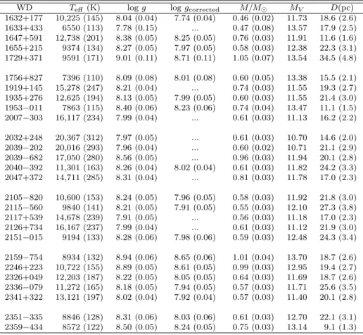
The spectroscopic log g values for the DA stars in the SDSS corrected in this fashion are displayed as a function of temperature in the bottom panel of Figure 2.15. The continuity of the log g distribution observed here through the entire temperature range suggests that our correction procedure appears reasonably sound. The corrected log g values for the cool DA stars in our local sample are reported in Table 2.3. Also given for each star are the corresponding stellar mass, absolute visual magnitude, and spectroscopic distance obtained from the distance modulus (V − MV = 5 log D− 5), where the V magnitudes are taken from
Table 2.1 and the MV values are calculated from model atmospheres at the spectroscopic values of Teff and (corrected) log g. All these quantities rely on the same evolutionary models
as before.
An external check of our correction procedure can be obtained by comparing the inferred masses for DA stars for which both photometric and spectroscopic estimates are available. This comparison is displayed in Figure 2.16 for spectroscopic masses derived for uncorrected as well as corrected log g values. We see that, overall, the photometric and corrected spectroscopic masses are in much better agreement, although in some cases the agreement is worse. There are also three objects at low photometric masses whose mass difference remains large. These are most likely unresolved double degenerates for which the inferred photometric masses are underestimated since the radius of these objects has been determined from the photometric technique under the assumption of a single star.
We finally point out that our log g correction procedure directly results in larger spectro-scopic distances, and as such, the number of stars in our local sample, defined within a given volume of space, might eventually be reduced.
2.5.5 Adopted Atmospheric Parameters
The final parameters for all white dwarfs in our sample are selected using the following criteria. For stars with Teff > 13, 000 K, spectroscopic solutions were systematically
pri-vileged over photometric solutions, when available. To avoid the high-log g problem below
Teff = 13, 000 K, photometric solutions were adopted, when available, and in the last resort, spectroscopic solutions corrected for log g were used. Since photometric analyses of stars with no trigonometric parallax measurements assume a value of log g = 8.0, these are only taken into account in the calculation of the luminosity function presented below, but not in the analysis of the mass distributions. All suspected or confirmed double degenerate systems are considered as single objects in what follows.
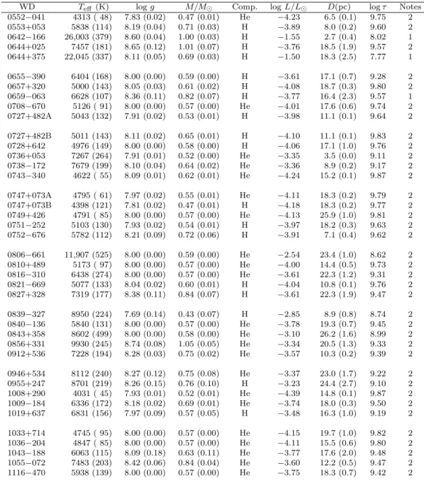
Our final results are presented in Table 2.4 where we give for each object the effective temperature (Teff), surface gravity (log g), stellar mass (M/M⊙), atmospheric composition
white dwarf cooling time (log τ ), and the method adopted to obtain these parameters.
2.6
Results
2.6.1 Distances
Based on the adopted photometric or spectroscopic distances presented in Table 2.4, we obtain a list of 133 objects for our final D < 20 pc sample, within the uncertainties. Before excluding from our sample any object beyond 20 pc, we make sure that the alter-nate distance estimate — either photometric or spectroscopic, when available — also places this object outside the 20 pc limit. A comparison of this final local sample with that defi-ned by Sion et al. (2009) reveals that 9 white dwarfs have been removed from the sample (0108+277, 0457−004, 0749+426, 0806−661, 0955+247, 1124+595, 1653+385, 1655+215, and 2336−079), while 16 have been included (0101+048, 0236+259, 0243−026, 0419−487, 0532+414, 0810+489, 0856+331, 1008+290, 1208+576, 1242−105, 2039−202, 2039−682, 2126 +734, 2248+293, 2347+292, and 2351−335). Note that the 3 white dwarfs without analyzable data (0208−510, 0415−594, and 1132−325) are not included in our analysis below but these are not necessarily excluded from the local sample. From this point on, when we refer to the local sample, we restrict ourselves to this list of 133 objects that have distance estimates inside the 20 pc region, within the quoted uncertainties.
2.6.2 Mass Distributions
The mass distribution as a function of effective temperature for each star in our sample is displayed in Figure 2.17. Atmospheric compositions and spectral types are indicated with different symbols. In particular, filled and open symbols represent hydrogen- and helium-rich compositions, respectively. For the hydrogen-rich stars, we also indicate which of the spectro-scopic or photometric method has been used (helium-rich stars all rely on the photometric method since there are no hot DB stars in our sample). Also superposed in this figure are the theoretical isochrones for our C/O core evolutionary models with thick hydrogen layers, as well as the corresponding isochrones with the main sequence lifetime added to the white
dwarf cooling age (for τ ≥ 2 Gyr isochrones only); here we simply assume (Leggett et al. 1998) tMS = 10(MMS/M⊙)−2.5 Gyr and MMS/M⊙ = 8 ln[(MWD/M⊙)/0.4]. As can be seen
from these results, white dwarfs with M . 0.48 M⊙cannot have C/O cores, and yet have been formed from single star evolution within the lifetime of the Galaxy. Some of these low-mass objects must either be unresolved double degenerates, or single white dwarfs with helium cores. In the former case, the stellar masses inferred from these figures are underestimated — especially if the unresolved components have comparable luminosities, and the corresponding cooling ages derived here become meaningless. The second possibility corresponds to single (or binary) helium-core degenerates whose core mass was truncated by Case B mass transfer before helium ignition was reached.
The objects displayed in red in Figure 2.17 are double degenerate binaries confirmed from radial velocity measurements: G1-45 (0101+048; Zuckerman et al. 2003), L870-2 (0135−052; Saffer et al. 1988), and L587-77A (0326−073; Zuckerman et al. 2003). The typical photometric masses inferred here for these systems are the order of∼ 0.3 M⊙, a direct consequence of the fact that we assumed that these stars are single objects, and thus overestimated their stellar radius by a factor of√2 (see equation 2.3), if both components are identical. Had we assumed two stars instead of one, a simple calculation yields photometric masses of∼ 0.58 M⊙, right in the bulk of normal white dwarfs. A good example of this calculation is for L870-2 (0135−052) with an extremely low photometric mass of 0.24 M⊙ (at Teff = 7260 K). Assuming two
identical DA stars yields instead 0.46 M⊙ for both components, in excellent agreement with the (corrected) spectroscopic mass of 0.48 M⊙ given in Table 3; the spectroscopic mass is not affected by the presence of two DA stars if they have comparable atmospheric parameters (see Fig. 1 of Liebert et al. (1991)). It turns out, indeed, that the two DA components in the L870-2 system are virtually identical (Bergeron et al. 1989). Hence, most, if not all low-mass stars observed in Figure 2.17 are probably unresolved double degenerates. However, a simple mass redetermination as prescribed above is not so simple. For instance, L532-81 (0839−327) with a spectroscopic mass of 0.43 M⊙ (at Teff = 8950 K) is already in perfect agreement with
its spectroscopic mass of 0.42 M⊙. In this particular case, assuming two DA stars would be the wrong thing to do, as this object appears to be a single DA star. We note, however, that