1. Goals of the SAPES project

(1)

Smart EMI monitoring of thin composites structures

Iccs16, Porto

Pierre Selva, Olivier Cherrier, Valérie Budinger , Frédéric Lachaud and Joseph Morlier

(2)

Overview

1. Goals of the SAPES project

2. Short focus on … our Multilevel approach and EMI experimental setup

3. Piezo properties identification by solving 3. Piezo properties identification by solving

inverse problem

4. Damaged zone localisation (Probabilistic Neural Networks)

5. Conclusion and future works

(3)

1.Goals

(4)

Structural Health Monitoring (SHM) method for in-situ damage detection and localization in Carbon Fibre Reinforced Plates (CFRP).

Impact detection in composites thin structures: in aeronautic Problem of Birdstrike, ice etc...

The detection is achieved using the ElectroMechanical Impedance (EMI) technique employing piezoelectric transducers as high-frequency modal sensors.

Goals

Numerical simulations based on the Finite Element (FE) method are carried out so as to simulate more than 100 damage scenarios.

Simple damage model is used in order to limit computation time (high discretization, high frequency bandwith) and from exploring all domain with few points (100) we construct an approximation (surrogate model using ANN) of damage localization versus selected (pertinent) indicators from EMI analysis.

Damage metrics are then used to quantify and detect changes between the

electromechanical impedance spectrum of a pristine and damaged structure

(5)

2.Short Focus on…

(6)

Short Focus on… Multilevel approach

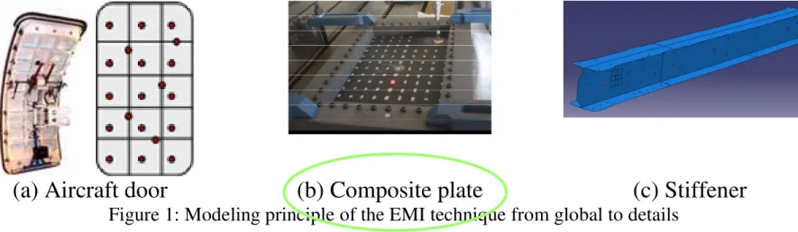
The main goal of his paper is to develop a multiscale localisation method that can be applied to a global structure (e.g. aircraft door), a subpart (composite plate) or a structural detail (stiffener).

The amount of data that needs to be generated to ensure a good generalization depends on the structure under study. For instance, if a global structure is considered, a large database of E/M impedance signatures relative to different localized single damage is ultimately required.

Simulations will be utilized so as to construct a significant database relative to the subpart problem in order that PNN well generalized (supervised approach)

(a) Aircraft door (b) Composite plate (c) Stiffener

Figure 1: Modeling principle of the EMI technique from global to details

ICCS16

(7)

Short Focus on… Modeling principle of the EMI

In order to generate a significant dataset relative to different damage localization

, a coupled-field finite-element (FE) model of the EMI technique is developed in Abaqus [8]

The FE model permits to compute electrical reaction charges over each sensor electrode,

which are then imported into Matlab [9] to derive the corresponding E/M impedance signature.

(8)

Short focus on … EMI measurement

PZT 2

Experimental setup

• 3 PZT mounted on composite plateT700 M21 (PI : PIC 151) : 10x10x0.5mm

• bi composants Epoxy/Argent (EPO-TEK® E4110) : thickness 0.3 mm

• Measurement system: Impedancemeter PsimetriQ N4L modèle 1700 + Active Head (integrated shunt

)

EMI principle:

→ Broadband excitation

- voltage measurement PZT

Plaque Composite

1 0

PZT 1 PZT 2

PZT 3

shunt shunt

PZT

R

I V ( )

)

( ω

ω =

) ( (

ω ω

PZT PZT

PZT

I

Z ) = V

- voltage measurement shunt - PZT intensity :

- Impedance estimation:

R_shunt

PZT

V_shunt

V_PZT

PSM 1700 PSM 1700

(9)

3.Piezo updating

(10)

Piezoceramics properties exhibit statistical fluctuations within a given batch and a variance of the order of 5-20% in properties

Therefore it becomes really important to accurately identify the behavior of the piezoelectric sensors as we solely depend upon these transducers to predict the mechanical impedance of the structure

Identification of piezo material properties solving inverse problem From experimental data

Fit Analytical model (Bhalla & Soh, 2004 & 2008)

Piezo updating (1)

Fit Analytical model (Bhalla & Soh, 2004 & 2008)

[ ]















=

T T T

T

33 11 11

0 0

ε ε ε

ε

[ ]

















=

0 0 0

0 0

0 0 0

33 31 31

15 15

d d d

d d

d ^η

Coef. diélectric Constants piezo. Structural

Damping )

1

33(

33^T ε^T δ i

ε = −

Coef.

Dielectric loss

Coef.

correction

C

Low freq ID(<10kHz) Around resonant

frequency ID (≈200kHz)

(11)

Impedance of a free PZT is :

Piezo updating (2)

Low Frequencies

¹

Bhalla & Soh (2004, 2008)

Exp measurements

2 linear functions of f

Identification of:

ε

₃₃^T

et δ

(12)

Example : PZT n°1

Piezo updating (2: results)

Résults for 3 PZT : Impedance Re(Z) of PZT n°1

bias due to non implemented dielectric losses in abaqus

(13)

Parameters to be identified:

Piezo updating (3)

C et d₃₁, η

Nonlinear quadratic function to be minimized

Analytic model

Exp

measurements

(14)

PZT n°1

Piezo updating (3: results)

Excellent numerical experimental correlation

It exists important difference between PZT manufacturer’s material data and identified data

(15)

4.0. The idea behind supervised ANN: generalization

(16)

Damaged zone identification

• Supevised ANN (previous studies) : discrete prediction (x,y) induce sometimes large errors

Pristine/damaged Plate

EM Impedance Abaqus or exp

Database of indicators.

ANN/PNN Detection

Localization -learning

-Test

Generalization is the process of recognize unknown cases from database of indicators (inputs) versus damage localisation (outputs)

• ICCS studies: Damaged zone prediction (classification problem well adapted to industrial constraints and multilevel approach)

Classification Problem PNN

(17)

PNN A simple example: 1 database of 4 examples (learning vectors)

weights

Z1 Z2

Z3 Z4

Plate divided in 4 zones

A¹ A² A³ A⁴

Radial Basis Layer Competitive Layer

















1 3 1 2 1 1

E E E

















=

3 ) / (

2 . 0 ) / (

5 . 1 ) / (

1 . 0 ) / (

4 3 2 1

A E d

r r r r

r r

































































4 3 4 2 4 1

3 3 3 2 3 1

2 3 2 2 2 1

1 3 1 2 1 1

A A A

A A

A Weights=learning

vectors A¹ A² A³ A⁴

d0 output¹









=

= 9 . 0

3 . 0

95 . 0

2 1

a a a

































































































0 0 1 0

0 0 0 1

0 1 0 0

0 0 0 1

A¹ A² A³ A⁴ Z1

Z2 Z3 Z4









=

= 3 . 0

1 . 0

63 . 0

2 1

b b b

Max probability predicted zone

y=Z1 x

Unknown case

E

r Classification

Matrix

Competitive Layer

(18)

4.1. Parametric approach (The big Picture)

(19)

Example : PZT n°1

4.1. Parametric approach (The big Picture)

PZT actuators/sensors

Damage of

Composite plate

PZT n°1 PZT n°2

PZT n°3

A finite-element model consisting of three piezoceramic patches (designation

PIC151) of dimensions 10x10x0.5mm

³

bonded onto a composite plate

(200x290mm

²

) .

The composite layup is composed of 12

plies of carbon/epoxy prepreg T700/M21

for a total thickness of 3mm.

(20)

Parametric approach (2)

Real (Z) (Oh ms) Real

(Z) (Oh ms)

UD D80%

D90% UD D90%

D80%

Damage surface of 255mm² Damage surface of 600mm²

(a) (b)

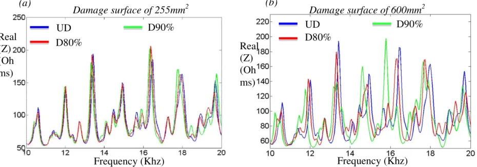
Figure 6. Comparison of impedance spectra predicted by the FE model at the PZT n°1 terminals between undamaged (UD) and damaged (D80% or D90%) composite plates. (a) and (b) Plots corresponding to a damage

surface of 225mm² and 600mm² respectively.

Frequency (Khz) Frequency (Khz)

(21)

• 3 damage zone surfaces: 100, 225, 600mm² 3 independant database

• 2 severities: decrease of 80% ou 90% de E

₂

/E

₃

/G

₁₂

/G

₁₃

/G

₂₃

• Border zones deleted from database

• Generation of database (learn 80%)

• Test of 100 networks (Results: mean of 5 best)

PNN Strategy : Mapping

• Cross (random) validation 20%

?

Pertinent indicators

Damage

localization

(x,y or zone)

(22)

PNN Preliminary tests

Inputs are defined from comparison of impredance spectrums (2 successive states :damaged/pristine)

• Corrélation Coef. (Re(Z))

• Area substraction (Re(Z) & Im(Z))

• Quadratic mean (Re(Z) & Im(Z))

• Root mean square deviation (Re(Z) & Im(Z))

Inputs choice is predominant in the classification results

1 2 2 2

[ ]

∑

⁻

=

N

i N

i

Z Z Zi

RMSD ₂

0 0 2

) Re(

)

Re( 7 indicators from

Bibliography for each PZT

21 indicators

Using only these indicators 47% of the networks are able to well classifiying 90% of the new damages

When we add 22 new indicators (frequency shifts)

85% of the networks are able to well classifiy 90% of the new damages

(23)

• As it can be expected, the higher the surface of damage, the higher the RMSD index is. The same conclusion can be drawn as regard the damage severity.

PNN Preliminary tests

Example of pertinent indicator RMSD

(24)

4.2. Database creation from numerical analysis

(Damage scenarii on Abaqus)

(25)

High damage area: 600mm²

Learning base 118 damages, no frequency shifts as input vectors

Test base 20 unlearned (new) cases

PNN

Random discrete location of damages

(26)

High damage area: 600mm²

PNN

69% of the networks can predict 90% of the unknonw (new) damage location

Dommages 600mm², sévérité d’endommagement 80%

90% f the networks can predict 80% of the unknown (new) damage location

10 new damages example

Very High variation of 21 indicators: can we reduce the input vector size ???

1/4 plate clustering

90% f the networks can predict 80% of the unknown (new) damage location

(27)

High damage area: 600mm²

PNN

PCA : reduced input vector containing RMSD Area diffrence of Re(Z) –

dimension 6 – has the same performance than the all vector : For High damage

area some indicators are correlated

(28)

Learning base 245 damages

Test base 20 unknown (new) cases

Medium damage area: 225mm²

PNN

Histogram (X and Y )

(29)

85% of the networks are able to predict 80% of the 20 new unknown damages

Medium damage area: 225mm²

PNN

85% of the networks are able to predict 80% of the 20 new unknown damages 61% of the networks are able to predict 90% of the 20 new unknown damages

Some examples

1/4 plate 20 examples

1/8 plate 20/20

(30)

Low damage area

Damages 100mm²

Learning base165 damages , Test base 20 unknown (new) cases

PNN

lower performance of the networks only of 35% of the networks are able to localize Indicators shifts are too small, database too small, local effects ?

PCA answers that all indicators are

needed …

(31)

4.3. Experimental results (unknown cases)

(32)

• Plate n°3:

Damage Localization

3 EMI curves

8,46%

7,34%

3,93%

PZT1 PZT2 PZT3

PZT 1 PZT 2

PZT 3

150

145

Défaut : S=277.63mm²

4.3. Experimental EMI

RMSD

Damage Localization

US and : Cscan resolution 0.3mm

Amplitude Profondeur

Données d’impact E=20J

Max

Déplacement

(mm) Effort (N) Temps d'impact (ms)

-5,63 6067,33 5,28

PZT1 PZT2 PZT3

20,00%

22,00%

21,00%

PZT1 PZT2 PZT3

Shift in frequency

(33)

4.4. Final Results of classification

Experimental constraints: central zone for impact drop test machine

So we only have 5 experimtal points

(unknown cases) to be recognized by the PNN

Plate n° Damage center (x,y)

US Surface Real zone Predicted zone

1 (150,145) ≈280mm² 2 2

2 (116,52) ≈381mm² 5 4

3 (110,87) ≈399mm² 5 5

4 (145,95) ≈380mm² 5 5

5 (177 ,105) ≈ 366mm² 2 4

(34)

5. Concluding remarks

EMI is able to detect and localize damage in composites plates, Our coupled FEM approach is interesting for exp/num EMI correlation

Piezo updating is an important phase in the monitoring process

3 surface of damages : 100, 225, 600mm² 3 different database, and 3 performances of PNN Supervised ANN x,y location prediction with reliability close to half damage size

PNN Damaged zones localization(1/4 ou 1/8 of plate)

Ability to predict correct zone for all kind of damages Good generalization for medium and large damage area

Futur works Increase of damage scenarii for better generalization (small damage area) Clustering of optimal zone (a priori information)

From ISO SURFACE NETWORKS to ISO ENERGY of IMPACT …

we need to know the predicted damage area versus location for each type of impact.