HAL Id: hal-00717366
https://hal.archives-ouvertes.fr/hal-00717366
Submitted on 12 Jul 2012
HAL is a multi-disciplinary open access
archive for the deposit and dissemination of
sci-entific research documents, whether they are
pub-lished or not. The documents may come from
teaching and research institutions in France or
abroad, or from public or private research centers.
L’archive ouverte pluridisciplinaire HAL, est
destinée au dépôt et à la diffusion de documents
scientifiques de niveau recherche, publiés ou non,
émanant des établissements d’enseignement et de
recherche français ou étrangers, des laboratoires
publics ou privés.
Semi-supervised NMF with time-frequency annotations
for single-channel source separation
Augustin Lefèvre, Francis Bach, Cédric Févotte
To cite this version:
Augustin Lefèvre, Francis Bach, Cédric Févotte. Semi-supervised NMF with time-frequency
annota-tions for single-channel source separation. ISMIR 2012 : 13th International Society for Music
Infor-mation Retrieval Conference, Oct 2012, Porto, Portugal. �hal-00717366�
SEMI-SUPERVISED NMF WITH TIME-FREQUENCY ANNOTATIONS
FOR SINGLE-CHANNEL SOURCE SEPARATION
Augustin Lef`evre
INRIA team SIERRA
Francis Bach
INRIA team SIERRA
C´edric F´evotte
LTCI/Telecom ParisTech
ABSTRACT
We formulate a novel extension of nonnegative matrix fac-torization (NMF) to take into account partial information on source-specific activity in the spectrogram. This infor-mation comes in the form of masking coefficients, such as those found in an ideal binary mask. We show that state-of-the-art results in source separation may be achieved with only a limited amount of correct annotation, and further-more our algorithm is robust to incorrect annotations. Since in practice ideal annotations are not observed, we propose several supervision scenarios to estimate the ideal mask-ing coefficients. First, manual annotations by a trained user on a dedicated graphical user interface are shown to provide satisfactory performance although they are prone to errors. Second, we investigate simple learning strate-gies to predict the Wiener coefficients based on local in-formation around a given time-frequency bin of the spec-trogram. Results on single-channel source separation show that time-frequency annotations allow to disambiguate the source separation problem, and learned annotations open the way for a completely unsupervised learning procedure for source separation with no human intervention.
1. INTRODUCTION
During the past decade, nonnegative matrix factorization (NMF) has become the core algorithm in single-channel source separation. A rich literature has been developed to adapt NMF to difficult scenarios in which sources are highly synchronized, and little or no development data is available.
In the past years, intensive research on Bayesian mod-elling and parameterized methods have been conducted to improve the identifiability of basis elements by restricting the complexity of the estimated model. More recently, an-other category of contributions consider incorporating in-formation that is directly relevant to the data at hand, and specified by the user. In [2], time activation of the sources is used to specify direct constraints on the activation coeffi-cients of the decomposition. Pitch estimates [5] were used
Permission to make digital or hard copies of all or part of this work for personal or classroom use is granted without fee provided that copies are not made or distributed for profit or commercial advantage and that copies bear this notice and the full citation on the first page.
© 2012 International Society for Music Information Retrieval.
for lead voice extraction. In [8], detailed score information is provided so that each individual note can be separated. While these contributions may use different NMF models, a common trait is that user information is used to spec-ify the support of decomposition coefficients at the coding stage. A quite different line of work is proposed in [1, 3], where isolated signals are used as proxy for the source sig-nals, so that information on both the basis functions and the activation coefficients can be used to constrain the fac-torization.
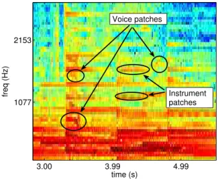
In this paper, we propose to annotate directly the time-frequency representation that is used to perform source separation. We assume that we are given recordings where a large fraction of time-frequency bins of the spectrogram may be assigned unambiguously to one dominant source. This hypothesis holds as long as there are not too many sources, and post-processing of the recording does not in-volve heavily non-linear effects. As illustrated in Figure 1, some patches in the spectrogram are cues for source-specific activity, which may be exploited as information on the optimal binary mask.
time (s) freq (Hz) 3.00 3.99 4.99 1077 2153 Instrument patches Voice patches
Figure 1: Cues from computational audio source analysis may be used as information on the optimal masking coef-ficients
In this article we make three contributions : we propose in Section 2 a novel modification of NMF (semi-supervised NMF) to take into account time-frequency annotations of the spectrogram, that is robust to errors in the annotations. In Section 2.3, we present a graphical user interface to re-trieve such time-frequency annotations. In Section 3, we
propose supervised learning algorithms to automatize an-notations, and explain how to combine them with semi-supervised NMF. Finally, we illustrate our contributions on publicly available source separation databases in Section 4.
2. SEMI-SUPERVISED NMF 2.1 Model and interpretation
In this section we propose a novel modification of NMF to incorporate annotations in the spectrogram. Let us first briefly summarize our NMF model and introduce mathe-matical notations, before proceeding to the main part of the contribution.
Given the short time Fourier transform of a signalX ∈ CF ×N
(in the followingf indexes frequency and n time), we assume thatX =PgS(g), whereS(g)∈ C
F ×N
is the spectrogram of each source signal forg ∈ {1, . . . , G}. De-fine the power spectrograms of the sourcesVf n(g)= |S(g)|2.
They are assumed to follow a linear model : Vf n(g)= PKg k=1W (g) f kH (g) kn, whereW(g)∈ R F ×Kg + ,H(g)∈ RKg×N. DefineK =P gKg,W = (W(1), . . . , W(G)) ∈ RF ×K + and H ⊤ = ((H(1))⊤ , . . . , (H(G))⊤ ) ∈ RK×N+ .
Then, depending on the assumed distribution of S(g),
es-timation ofW and H amounts to minimizing d(V, W H) whered is a measure of fit between data and the under-lying model. In this article we will use the Itakura-Saito divergence, but actually anyβ-divergence may be used.
Given estimates ˆVf n(g)of the power spectrogram of each source, time domain estimates of the sources are then com-puted by Wiener filtering, where the Wiener coefficients of the source in the time-frequency domain are given by : Mf n(g)=
ˆ Vf n(g)
ˆ Vf n.
The key idea in our contribution is the following : sup-pose we have at hand a setL of annotated time-frequency bins and a set of time-frequency masksMf n(g) such that :
Mf n(g)∈ [0, 1], and P gM (g) f n = 1 if (f, n) ∈ L, P gM (g) f n = 0 otherwise.
For annotated time-frequency bins, we define target val-ues for each source spectrogram : ˜Vf n(g)= M
(g) f nVf n.
The remaining, un-annotated entries of ˆV are then com-puted so as to fit the observed spectrogram. This idea trans-lates into the following optimization problem :
minX (f,n) dIS(Vf n, ˆVf n) + λ X (f,n)∈L g=1,...,G µf ndIS( ˜Vf n(g), ˆV (g) f n ) , (1) wheredIS(x, y) = xy−logxy−1 is the Itakura-Saito
diver-gence1, and optimization is subject to the constraints that W ≥ 0 (point-wise nonnegativity), H ≥ 0, andPfWf k =
1 to avoid scaling ambiguity. We interpret the second term in Eq. (1) as a relaxed version of the constraints that ˆVf n(g)
be equal to their target value Mf n(g)Vf n, for all annotated
bins(f, n) ∈ L.
1Given that some values are set to zero, we replace the IS divergence
dI S(x, y) by dI S(ǫ + x, ǫ + y) (where ǫ = 10−7) in our optimization
problem, in order to deal with ill-conditioning of the objective function.
We may tune the relative importance of annotation by varying parameterλ, from λ = 0 (standard NMF), to λ → +∞ (in which case (W H)f n = Vf n(g)is enforced exactly
if there are any feasible solutions). Thus, robustness to uncertainty in the annotations is introduced by replacing hard constraints by penalty terms in the NMF optimization problem. Note that since annotations dictate the assign-ment of components to sources, there is no need to group components by hand. We will discuss the role ofµf n in
the next section : in the case of user annotations,µf n= 1.
Let us discuss two cases :
(a) M(g)fn ∈ {0, 1}: this is the case of user annotations, where time-frequency bins are labelled by hand. In this case, there can be only one active source at each time-frequency bin, since PgMf n(g) = 1. This is a strong as-sumption, which is verified for a large fraction of the mix-tures that are found in blind source separation.
(b) M(g)fn ∈ [0, 1]: this general case is relevant to the
learn-ing procedures we introduce in the next section, since they output decision values in[0, 1].
Discussing the algorithm is beyond the scope of this pa-per : we used a multiplicative updates algorithm with ap-propriate modifications to deal with the additional terms in Eq. (1) [6].
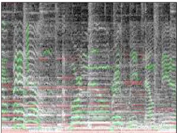
Figure 2: Example of user annotations in a ten seconds’ audio track: green regions are assigned to voice, and red regions to accompaniment (best seen in color).
2.2 Relation with previous work
As in [2, 8, 5], annotations are used to constraint some sources to be inactive. In fact, time annotations are a spe-cial case of our model, where annotations are such that Mf n(g)= M
(g)
f′nfor all(f, f ′
) (i.e., zeroes come in columns). Our model deals with that case when there are two sources. The only difference between our model and [2] is that in-stead of enforcingHkn = 0 as a hard constraint, we
in-troduce a soft penalty to enforceWf kHkn = 0, with the
added benefit that incorrect annotations are dealt with in a robust fashion. The case of more than two sources is dealt with a simple extension of Eq. (1), which we omit here for lack of space.
2.3 A graphical user interface for time-frequency annotation of spectrograms
In this section, we investigate manual annotation of the spectrogram. A GUI was designed in Matlab to anno-tate spectrograms (see Figure 2), with some extra sound functionalities to help the user. It takes sound files as in-put, applies some basic preprocessing (re-sampling at user-specified rate, down-mixing to mono), computes a time-frequency representation via user-specified parameters, and displays the spectrogram. Zooming and slide-rule navi-gation are enabled for better visualization. Annotation of sources is done with a simple rectangle drawing utility : one color for each source, as illustrated in Figure 2. An-notations are stored in an annotation mask of dimension F × N × G (where (F, N ) is the size of the spectrogram andG the number of sources). Several annotation masks may be loaded into memory and displayed alternatively, so the user can compare, for instance, manual annotations with the output of a blind source separation algorithm. An-notation masks may be exported to .mat format for further processing. Finally, we implemented playback functional-ities to help the user annotate the spectrogram.
We designed the GUI to make the annotation process easier and faster : indeed, in our experience, while time an-notations are easy and require only listening once or twice to the mix, time-frequency annotations are hard even for trained users : it takes up to one hour to annotate20% of a twenty seconds track.
3. TOWARDS A SUPERVISED ALGORITHM FOR ANNOTATION
Research in computational audio scene analysis (CASA) has emphasized the role of frequency tracks in source iden-tification : indeed by looking at a spectrogram, it is easy to assign a significant number of frequency tracks either to a voiced source or a musical source (see Figure 1). In previ-ous works, such cues have been used to compute a similar-ity matrix that would then be used to perform clustering see [9, 4]. We propose here a supervised learning procedure to predict annotations automatically. At train stage, we have at hand separate sources so that we observe not only the mix, but also the Wiener coefficientsMf n(g) computed on
the ground truth, while at test stage we only observe V . Thus, the goal is to predict E(M(g)|V ). In order to
allevi-ate the computational burden2, we make two restrictions
on the learning procedure : each vector(Mf n(1), . . . , M (G) f n )
for a given time-frequency bin (f, n) is predicted inde-pendently of the others, and based only on the values of patches centered at that time-frequency bin.
We now introduce the features and algorithms used to train our predictor.
3.1 Features
The basic input to our learning algorithms consists in rect-angular time-frequency blocks extracted from the input power
2indeed even for ten seconds’ excerpts, there are more than500 ×
1000 time-frequency bins for standard STFT parameters
100 101 102 103 10−1 100 101 102 103 104 105 106
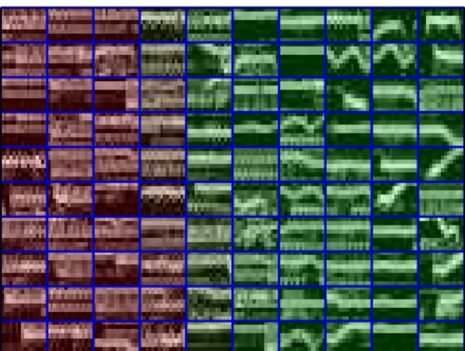
Figure 3: Samples of patches extracted from the SISEC database. Intensity reflects amplitude, patches which are labeled as accompaniment are in red, while patches which are labeled as voice are in green. Patches in brown have mixed Wiener coefficients (best seen in color).
spectrogram. The size of the rectangular blocks is fixed as a parameter of the algorithm. They are then normalized to have unitℓ1-norm so the features are scale invariant. We
also considered taking the log of patches, adding coordi-nates of the patch as additional information, and taking a Gabor transform of the patches. The Gabor transform in particular was introduced so that correlations between pix-els in each time-frequency blocks is taken into account. Finally, we also tried averaging the ground truth Wiener coefficients before learning, so that predicted regression surfaces are smoother in time-frequency space.
3.2 Learning algorithms
Due to space limitation, we restrict ourselves to naming the algorithms we chose and highlighting the key parame-ters to tune. We refer the reader to standard textbooks on machine learning for more details (e.g., [7]).
K-nearest neighbors (knn): for each test pointx(test)i , the
C nearest points x(train)j ,j ∈ {1, . . . , C} from the train set
are used to predictMi(g)= 1/C
P
jM (g) j .
Quantized knn (km): We learnC clusters from the train set using K-means; for each cluster, we compute average prediction coefficientsMc(g). For each test point, we
pre-dictMc(g)from the nearest clusterc.
Random Forests (rf): We learnC regression trees of depth d from the train set and average over the C predictions for each test point.
We will refer to this supervised learning procedure as automatic annotations, no matter which algorithm is used. 3.3 Computation ofµf nfor automatic annotations
While the learning algorithms presented above predict Wie-ner coefficients, output values near0.5 reflect uncertainty in the Wiener coefficients rather than prediction of mixed volumes. For this reason we introduce an additional tun-ing parameterµf nin Eq. (1), so that output values near0.5
are less taken into account than values near{0, 1}. As a rule, we chooseµf n = 1 −G−1G P gM (g) f n(1 − M (g) f n), so
that 0 ≤ µf n ≤ 1 and µf n = 0 if all Mf n(g)are equal.
Moreover, when annotations are in{0, 1}, we always have µf n = 1.
4. EXPERIMENTAL RESULTS 4.1 Description of music databases
We used two publicly available databases in our experi-ments: the QUASI database3 and the SISEC database for
Professionally Produced Music Recordings4. All source tracks were down-sampled from 44100 Hz to 16000 Hz, and down-mixed to mono by taking the average of left and right channels. A voice track and accompaniment track are then created by aggregating the various source files, and then a final mix is created by summing the two tracks. Sine-bell windows of size1024 with 512 overlap were used to compute short time Fourier transforms. The QUASI database contains longer tracks that are amenable to time annotations. The SISEC database contains short tracks where only time-frequency annotations can be used. Al-though detailed instrumental tracks are provided for most of the mixtures, we work only on single-channel signals. Since we are dealing with under-determined mixtures, we restrict ourselves to separating voice from accompaniment in each track, in order to alleviate the difficulty of the prob-lem.
4.2 Ideal performance of semi-supervised NMF and robustness to wrong annotations
SDR1 SDR2 SIR1 SIR2 SAR1 SAR2 0.1 % -0.02 -0.60 5.15 5.16 3.62 2.33
1 % 0.70 0.24 4.59 6.25 4.39 2.85 10 % 6.71 6.68 13.57 16.53 7.95 7.40 100 % 10.40 10.41 19.88 20.88 11.00 10.88
Table 1: Mean results on the SISEC database, as the pro-portion of annotation increases.
Table 1 displays source separation results achieved by semi-supervised NMF on the SISEC database when fed with the actual Wiener coefficients computed from the ground truth sources. Source separation performance is measured by Source to Distortion Ratio (SDR), Source to Interfer-ence Ratio (SIR), and Source to Artefact Ratio (SAR). Higher values indicate better performance. As we can see, sat-isfactory results are obtained with as little as10% of an-notations. When 100% of annotations are given, NMF does nothing and the computed masks are simply the ideal Wiener coefficients computed from the sources.
We study the robustness of our NMF routine by replac-ing part of the ideal annotations by noise to simulate hu-man errors. Table 2 displays average SDRs obtained when fixing the annotation rate to10% and varying either the rate
3www.tsi.telecom-paristech.fr/aao/ 4sisec.wiki.irisa.fr
wrong annotationsp or the optimization parameter λ. As expected, for fixedλ the average SDR drops as p increases. Whenp is fixed, there is an optimal value of λ that trades off the benefits and drawbacks of annotations. Fixing the target annotation rate to10%, satisfactory results are ob-tained with up to10% of wrong annotations (i.e.1% of the spectrogram). λ p = 0 p = 0.05 p = 0.1 p = 0.2 p = 0.5 10−1 0.11 -0.08 -1.76 -1.47 -1.47 100 5.59 4.10 3.50 2.29 1.20 101 7.59 6.53 5.32 3.43 0.59 102 7.07 5.66 4.54 3.15 0.77
Table 2: Mean SDR value as λ and the proportion of wrong annotations vary. The proportion of annotations is set to0.1
4.3 Automatic annotation : comparison of algorithms and experimental results
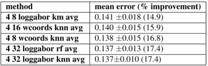
method mean error (% improvement) 4 8 loggabor km avg 0.141±0.018 (14.9)
4 16 wcoords knn avg 0.140±0.015 (15.9) 4 8 wcoords knn avg 0.138±0.015 (16.8) 4 32 loggabor rf avg 0.137±0.013 (17.4) 4 32 loggabor knn avg 0.137±0.010 (17.4)
Table 3: Mean error on Wiener coefficient predictions on the SISEC database (% improvement over random predic-tion), for various learning strategies .
Learning algorithms were trained by dividing the SISEC database in two sets of tracks. For each set, we train detec-tors and test them on the other set. Thus we may compute annotations and run semi-supervised NMF for all tracks without the risk of overfitting. We emphasize the fact that each track is annotated with a detector that has never seen the spectrogram before : our method is purely supervised with no adaptation to test data. Parameters of the learning algorithms were selected at train stage by cross-validation. Time-frequency patches of size in{4, 8}×{8, 16, 32} were extracted. Out of each track we extract5 × 103patches at
train time, and105patches a test time, so approximately
10% of the track is annotated at test time when semi-super-vised NMF is called.
We display in Table 3 the results of the best 5 detec-tors, in terms of mean prediction error (first column) and in terms of relative improvement over a purely random predictor. Detectors are named after the following rule : {patch size} {feature} {learning method} {averaging or identical}. For instance, the tag loggabor corresponds to taking log then Gabor transform of patches, and wcoords adding frequency coordinates of the patches as side infor-mation. Note that we used exact Wiener coefficients to compute errors, so that all detectors can be compared even when averaging was used at train stage. The improvement over a random predictor is consistent across the features and the algorithms that were used. Figure 4 compares an-notations provided by the best detectors from Table 3 with
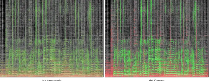
(a) Automatic (b) Correct
Figure 4: Comparison of automatic annotations and correct annotations (at the same time-frequency bins). Gray-scale time-frequency bins are not annotated, red bins are annotated as accompaniment, green bins as voice(best seen in color). ideal annotations at the same points were automatic
anno-tations were made. Red time-frequency bins correspond to accompaniment, and green to voice. The most strik-ing observation is that, while ideal annotations are in very bright colors (few Wiener coefficients are different from0 or 1), automatic annotations, on the other hand, are gen-erally biased towards 0.5. This is to be expected since predicting0.5 incurs a risk of losing at most 0.25 (since we use a regression loss), while predicting 0 or 1 incurs a maximum loss of 1. The main asset of automatic an-notations is that pitch tracks with varying frequency are successfully predicted as voice. Automatic annotations are biased towards predicting voice in the higher frequencies : however the learning algorithm in this example did not have the information of frequency. This might be because transients “look” a lot like patches of unvoiced speech. Fi-nally, one may spot inconsistencies in the predictions in the sense that points belonging to the same pitch tracks are sometimes classified incoherently, which is not surpris-ing since the learnsurpris-ing algorithms we have proposed predict time-frequency bins independently.
To sum up, predictions of Wiener coefficients from lo-cal patches are not perfect but provide a good starting point for further modelling of the spectrogram. We expect that better performance could be obtained by using more ad-vanced cues from CASA, such as pre-clustering the spec-trogram into pitch tracks and transient tracks, before learn-ing5.
4.4 Overall results
We now turn to results obtained by semi-supervised NMF combined with various annotation methods. On the SISEC database, manual time-frequency annotations were done with the GUI presented in Section 2.3. On the QUASI database, tracks were amenable to significant time
anno-5This is very similar to what is done in vision, where super-pixels
help deal with consistency in prediction and alleviate the computational burden of predicting all pixel values.
tations, so by comparing results on both databases we can compare the respective benefits of time-frequency annota-tions VS time annotaannota-tions.
In both scenarios, we compare five methods :
auto : Automatic annotations and semi-supervised NMF. The best detector from Table 3 was chosen.
user : User annotations and semi-supervised NMF (time-frequency annotations for SISEC, manual annotations for QUASI). We triedK ∈ {5, 10, 20} for the SISEC database and{10, 20, 50} for the QUASI database, as well as λ ∈ {1, 10, 100}, and selected parameters yielding highest SDR for fair comparison with the baseline.
baseline : Run NMF and permute factors to obtain op-timal SDR. We setK = 8 because it already takes a 10 times as long to evaluate SDRs for all permutation on a single track as it takes to run semi-supervised NMF. self : sets(g)= 1
Gx as estimates for the sources, it serves
to estimate the difficulty of the source separation problem for a given database.
oracle : results obtained with Wiener coefficients com-puted from the ground truth. In addition we display track by track annotation accuracy for user annotations, for com-parison with Table 2. For each method, we ran NMF three times for 1000 iterations to avoid local minima, and kept the run with the lowest objective cost value.
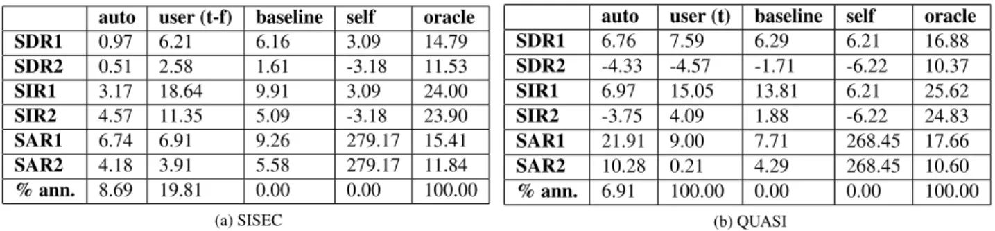
Tables 5a and 5b display average evaluation metrics for each source (source 1 is always the accompaniment, and source 2 is always the voice), on two different databases :
% annotated % correct track 1 0.23 0.91 track 2 0.10 0.89 track 3 0.29 0.91 track 4 0.17 0.81 track 5 0.22 0.95
Table 4: Evaluation of user annotations on the SISEC database.
auto user (t-f) baseline self oracle SDR1 0.97 6.21 6.16 3.09 14.79 SDR2 0.51 2.58 1.61 -3.18 11.53 SIR1 3.17 18.64 9.91 3.09 24.00 SIR2 4.57 11.35 5.09 -3.18 23.90 SAR1 6.74 6.91 9.26 279.17 15.41 SAR2 4.18 3.91 5.58 279.17 11.84 % ann. 8.69 19.81 0.00 0.00 100.00 (a) SISEC
auto user (t) baseline self oracle SDR1 6.76 7.59 6.29 6.21 16.88 SDR2 -4.33 -4.57 -1.71 -6.22 10.37 SIR1 6.97 15.05 13.81 6.21 25.62 SIR2 -3.75 4.09 1.88 -6.22 24.83 SAR1 21.91 9.00 7.71 268.45 17.66 SAR2 10.28 0.21 4.29 268.45 10.60 % ann. 6.91 100.00 0.00 0.00 100.00 (b) QUASI
Table 5: Results on the evaluated databases: (a) time-frequency annotations, (b) time annotations.
on the SISEC database, we experimented with time-fre-quency annotations since the tracks were too short for time annotations. Overall, results on the SISEC database are better than those on QUASI. Our interpretation is that since most of the time the accompaniment is active, the dictio-naries tend to overfit the accompaniment and underfit the voice. Time-frequency annotations on SISEC yield SDRs that are a few points below that predicted by our bench-mark from Table 2 : indeed human errors are not dis-tributed randomly as was the case in our benchmark. Time-frequency annotations outperform the baseline by1 point in SDR, which is significant because in semi-supervised NMF there is no manual grouping of the components. Time annotations loose to the baseline by−1 in SDR, but they are still significantly correlated with the true sources when compared with the baseline.
On the SISEC database, automatic annotations are also below the baseline, however they are also significantly cor-related with the true sources, when compared with the “self” column. Signal to Interference Ratios are even comparable with those of the baseline on the SISEC database. Auto-matic annotations do not perform as well on the QUASI database since we trained detectors only on tracks from SISEC, so that more supervision would significantly im-prove those figures.
To conclude, we have shown that time-frequency anno-tations can improve significantly over NMF with ideally grouped components. On longer tracks, time only anno-tations yield reasonable results, but even when 100% of the track is annotated, the estimated sources contain strong interferences. Automatic annotations yield similar results, but leave considerable room for improvement, since with time-frequency annotations there will always be a point where enough annotations with limited errors will provide audible estimates of the sources.
5. CONCLUSION
We have proposed a novel formulation of semi-supervised NMF that successfully takes into account annotations to enhance the discriminative power of NMF. Semi-supervised NMF is defined so that when a certain amount of annota-tions is reached, source separation quality is near that of ideal binary masks. Manual annotations retrieved with our graphical user interface yield satisfactory results. We are
investigating ways to define annotations independently of the particular time-frequency representation that is used.
Finally, semi-supervised NMF opens the way for inter-action with methods from computational audio scene anal-ysis. As such, the simple features and textbook pattern matching algorithms we have presented show promising results.
6. REFERENCES
[1] P. Smaragdis and G. Mysore. “Separation by “hum-ming”: User-guided sound extraction from mono-phonic mixtures.”, WASPAA, 2012.
[2] B. Wang. “Musical Audio Stream Separation”, Msc Thesis, 2009.
[3] D. Fitzgerald. “User Assisted Source Separation using Non-negative Matrix Factorisation”, Irish Signals and Systems Conference, 2011.
[4] F. Bach and M.I. Jordan. “Blind one-microphone speech separation: a spectral learning approach.” NIPS, 2004.
[5] J.-L. Durrieu and J.-P. Thiran. ”Musical audio source separation based on user-selected f0 track.” (LVA/ICA), 2012.
[6] C. F´evotte, N. Bertin, and J.-L. Durrieu. ”Nonnegative matrix factorization with the Itakura-Saito divergence: With application to music analysis.” Neural Computa-tion, 2009.
[7] T. Hastie, R. Tibshirani, and J. Friedman. The elements of statistical learning. Springer, 2nd edition edition, 2009.
[8] R. Hennequin, B. David, and R. Badeau. ”Score in-formed audio source separation using a parametric model of non-negative spectrogram.” ICASSP, 2011. [9] M. Lagrange, L.G. Martins, J. Murdoch, and G.
Tzane-takis. ”Normalized cuts for predominant melodic source separation.” TASLP, 2008.