HAL Id: hal-01074090
https://hal.archives-ouvertes.fr/hal-01074090
Submitted on 12 Oct 2014
HAL is a multi-disciplinary open access
archive for the deposit and dissemination of sci-entific research documents, whether they are pub-lished or not. The documents may come from
L’archive ouverte pluridisciplinaire HAL, est destinée au dépôt et à la diffusion de documents scientifiques de niveau recherche, publiés ou non, émanant des établissements d’enseignement et de
Combining Face Averageness and Symmetry for
3D-based Gender Classification
Baiqiang Xia, Boulbaba Ben Amor, Hassen Drira, Mohamed Daoudi,
Lahoucine Ballihi
To cite this version:
Baiqiang Xia, Boulbaba Ben Amor, Hassen Drira, Mohamed Daoudi, Lahoucine Ballihi. Combining Face Averageness and Symmetry for 3D-based Gender Classification. Pattern Recognition, Elsevier, 2015, 48 (3), pp.746-758. �hal-01074090�
Combining Face Averageness and Symmetry for
3D-based Gender Classification
Baiqiang Xia, Boulbaba Ben Amor, Hassen Drira, Mohamed Daoudi, and Lahoucine Ballihi.
Abstract
Although human face averageness and symmetry are valuable clues in so-cial perception (such as attractiveness, masculinity/femininity, healthy/sick, etc.), in the literature of facial attribute recognition, little consideration has been given to them. In this work, we propose to study the morphologi-cal differences between male and female faces by analyzing the averageness and symmetry of their 3D shapes. In particular, we address the following questions: (i) is there any relationship between gender and face average-ness/symmetry? and (ii) if this relationship exists, which specific areas on the face are involved? To this end, we propose first to capture densely both the face shape averageness (AVE) and symmetry (SYM) using our Dense Scalar Field (DSF), which denotes the shooting directions of geodesics be-tween facial shapes. Then, we explore such representations by using classical machine learning techniques, the Feature Selection (FS) methods and Ran-dom Forest (RF) classification algorithm. Experiments conducted on the FRGCv2 dataset show a significant relationship exists between gender and facial averageness/symmetry when achieving a classification rate of 93.7% on the 466 earliest scans of subjects (mainly neutral) and 92.4% on the whole
FRGCv2 dataset (including facial expressions). Keywords:
3D Face, Gender Classification, Face averageness, Face symmetry, Dense Scalar Field, Feature selection, Random Forest.
1. Introduction
1
Human gender perception is an extremely reliable and fast cognitive
pro-2
cess since the face presents a clear sexual dimorphism [1]. In human face
3
analysis using machines [3], automatic gender classification is an active
re-4
search area. Developed solutions could be useful in human computer
in-5
teraction (intelligent user interface, video games, etc.), visual surveillance,
6
collecting demographic statistics for marketing (audience or consumer
pro-7
portion analysis, etc.), and security industry (access control, etc.). Research
8
on automatic gender classification using facial images goes back to the
begin-9
ning of the 1990s. Since then, significant progress has been reported in the
10
literature [4, 5, 6, 7, 8]. Fundamentally, proposed techniques differ in (i) the
11
format of facial data (2D still images, 2D videos or 3D scans); (ii) the choice
12
of facial representation, ranging from simple raw 2D pixels or 3D cloud of
13
points to more complex features, such as Haar-like, LBP and AAM in 2D,
14
and shape index, wavelets and facial curves in 3D; and (iii) the classifiers,
15
for instance Neural Networks, SVM, and Boosting methods [4].
16
1.1. Related work on 3D-based gender classification
17
Statistically, the male and the female faces present different morphological
18
characteristics in geometrical features, such as in the hairline, the forehead,
19
the eyebrows, the eyes, the cheeks, the nose, the mouth, the chin, the jaw, the
neck, the skin and the beard regions [13]. Usually, the female brow tends to be
21
more arched than that of the male (which is more horizontal), the noses and
22
chins in male faces are more prominent than those in female faces [27], and
23
men have a more acute nasolabial angle than women [26]. The 3D face scans,
24
which capture the spatial structure of the facial surfaces, allow to capture
25
these differences between male and female faces more easily compared to 2D
26
texture images. Thus, the goal of 3D-based gender classification is to develop
27
a fast and automatic approach which yields high classification performance
28
compared to the 2D-based approaches.
29
In [9], Liu et al. analyze the relationship between facial asymmetry and
30
gender. They impose a 2D grid on each 3D face to represent the face with
31
3D grid points. With the selected symmetry plane, which equally separates
32
the face into right and left halves, the distance difference between each point
33
and its corresponding reflected point is calculated as height differences (HD).
34
In addition, the angle difference between their normal vectors is calculated
35
as orientation differences (OD). The approach based on HD-face achieves
36
91.16% and the approach based on OD-face achieves 96.22%. However, these
37
performances are reported on a private dataset of 111 full 3D neutral face
38
models of 111 subjects, and 3D face manual landmarks are needed.
39
In [12], Lu et al. use Support Vector Machine (SVM) to classify ethnicity
40
(Asian and Non-Asian) and gender (Male and Female). A merging of two
41
frontal 3D face databases (UND and MSU databases) is used for the
exper-42
iments. The best gender classification results using 10-fold cross-validation
43
reported is 91%. However, this approach is based on six landmarks (inside
44
and outside corners of the eyes, the nose tip, and the chin point) manually
labeled. Moreover, the results are obtained only on neutral faces.
46
In [15], Wu et al. use 2.5D facial surface normals recovered with Shape
47
From Shading (SFS) from intensity images for gender classification. The
48
best average gender recognition rate reported is 93.6% with both shape and
49
texture considered. However, seven manual landmarks are needed and a
50
small dataset of neutral scans has been used to perform the experiments.
51
In [16], Hu et al. propose a fusion-based gender classification method
52
from 3D frontal faces. Each 3D face shape is separated into four face regions
53
using face landmarks. With the extracted features from each region, the
54
classification is done using SVM on a subset of the UND dataset and another
55
database captured by themselves. Results show that the upper region of
56
the face contains the highest amount of discriminating gender information.
57
Fusion is applied to the results of four face regions and the best result reported
58
is 94.3%. Their experiments only involve neutral faces. In this study, no
59
attention is given to facial expressions.
60
In [3], Toderici et al. employ MDS (Multi-Dimensional Scaling) and
61
wavelets on 3D face meshes for gender classification. They use the 4007
62
3D scans of the 466 subjects from the FRGCv2 dataset for gender
classifi-63
cation. Experiments are carried out subject-independently with no common
64
subject used in the testing stage of 10-fold cross validation. With polynomial
65
kernel SVM, they achieve 93% gender classification rate with the
unsuper-66
vised MDS approach, and 94% classification rate with the wavelets-based
67
approach. Both approaches significantly outperform the kNN and
kernel-68
kNN approaches.
69
In [17], Ballihi et al. extract facial curves (26 level curves and 40 radial
curves) from 3D faces for gender classification. The features are extracted
71
from lengths of geodesics between facial curves from a given face to the Male
72
and Female templates computed using the Karcher Mean Algorithm. The
73
Adaboost algorithm is then used to select salient facial curves. They obtained
74
a classification rate of 84.12% with the nearest neighbor classifier when using
75
the 466 earliest scans of the FRGCv2 dataset as the testing set. They also
76
performed a standard 10-fold cross-validation for the 466 earliest scans of
77
FRGCv2, and obtain 86.05% with Adaboost.
78
Compared to [17], in the current paper, we represent mathematically
fa-79
cial bilateral symmetry and averageness for gender classification using Dense
80
Scalar Fields. The DSFs denoting the shooting directions for geodesics
be-81
tween facial shapes, are both novel and interesting. We view this
representa-82
tion for gender classification as the main contribution of this paper. The set
83
of facial deformations is a nonlinear space while the set of Dense Scalar Field
84
(DSF) is a vector space. The only remaining challenge is the large
dimen-85
sionality of DSF, which is handled using a feature-selection-based dimension
86
reduction, followed by a Random Forest classifier. In terms of experimental
87
performances, the present approach have achieved higher classification rates
88
compared to [17]. In summary, the novelty of this paper is in
represent-89
ing bilateral symmetry and face averageness using DSF and its successful
90
application to the gender classification problem.
91
1.2. Methodology and contributions
92
From the above analysis, existing works on 3D-based gender classification
93
are based on local or global low-level feature extraction (see table 2 for a
94
complete summary) followed by classical classification methods. To the best
of our knowledge, no work has been done considering high-level cues, such as
96
face averageness and bilateral face symmetry, except the study in [9] which
97
investigates the relationship between facial symmetry and gender. Using
98
sparse measures of height differences (HD), and orientation differences (OD)
99
on a defined grid imposed on full 3D face models, their process requires
100
manual landmarks on the face and the experiments are performed on a small
101
dataset. The main contributions of this work are as follows :
102
☞ We introduce two high-level features, face averageness (AVE) and
bilat-103
eral face symmetry (SYM), for 3D-based gender classification. These
104
primary facial perception features are rarely considered in the literature
105
of facial attribute recognition.
106
☞ We provide an interesting mathematical tool, named Dense Scalar
107
Field (DSF) [18], to capture densely and quantitatively the
average-108
ness/symmetry differences on the face surface. The DSFs grounding on
109
Riemanniann shape analysis are capable to densely capture the shape
110
differences in 3D faces (such as averageness/symmetry differences).
111
☞ We propose a fully-automatic gender classification without any
hu-112
man interaction. We achieve competitive results compared to the
113
approaches in the state-of-the-art on a challenging dataset, FRGCv2.
114
Also, we provide a comprehensive study of the robustness of the
pro-115
posed approach against age, ethnicity and expression variations.
116
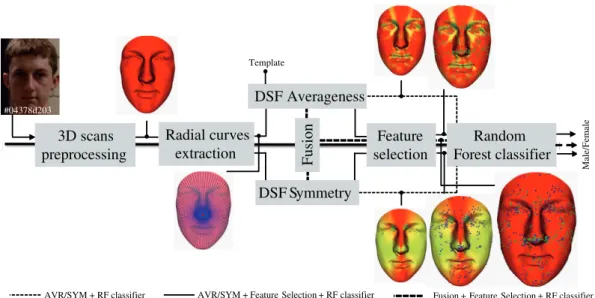
An overview of the proposed approach is shown in Figure 1. Firstly,
dur-117
ing the first step an algorithm commonly used for facial scans preprocessing is
118
applied. Its includes hole filling, facial part cropping and 3D mesh smoothing
3D scans preprocessing Radial curves extraction DSF Averageness Feature selection Random Forest classifier DSF Symmetry F u si on M al e/ F em al e Template #04378d203
AVR/SYM + RF classifier AVR/SYM + Feature Selection + RF classifier Fusion + Feature Selection + RF classifier Figure 1: Flow chart of the proposed gender classification approach. There are various pipelines for gender classification. Namely, the pipelines are, (1) the symmetry DSF features (SYM-Original), (2) the selected features of symmetry DSF features (SYM-Selection), (3) the averageness DSF fea-tures (AVE-Original), (4) the selected feafea-tures of averageness DSF feafea-tures (AVE-Selection), (5) the fusion of symmetry and averageness DSF features by concatenation (FUS-Original), and (6) the selected features of the fusion of symmetry and averageness DSF features (FUS-Selection).
applied to each scan, together with nose tip detection and pose
normaliza-120
tion, as proposed in [17] or [12]. We denote the preprocessed face as S. The
121
plane which equally separates the preprocessed face S into right and left
122
halves is picked up as the middle plane. This plane P (t, −n→h) passes through
123
the detected nose tip t and has a horizontal normal −n→h from the frontal view.
124
Secondly, a DSF extraction step goes after the preprocessing. Here, the
pre-125
processed face S is approximated by a collection of radial curves defined over
126
the facial region and stemming from the nose tip. Then, the Dense Scalar
127
Field (DSF) features are computed, pair-wisely, to capture the shape
ferences (averagenesss/symmetry differences) between corresponding radial
129
curves on each indexed point. Thus, we obtain two DSFs for each scan, an
130
averageness DSF and a symmetry DSF. A fusion descriptor is then obtained
131
for each scan by concatenating its averageness DSF and symmetry DSF.
132
Thirdly, after DSF extraction, we investigate the two following classification
133
pipelines. In the first pipeline, Random Forest classifier is applied directly
134
on the obtained feature vectors - averageness DSFs, symmetry DSFs and
135
fusion DSFs. In the second pipeline, we first apply a supervised feature
se-136
lection (FS) algorithm on the averageness, symmetry and their fusion DSFs,
137
then the Random Forest (RF) classifier is applied on the selected features for
138
gender classification.
139
This work relates closely to the work previously published in [17], in terms
140
of face representation by an indexed collection of radial curves, which is one
141
of the first steps of our approach’s pipeline. However, while this face
param-142
eterization is in common, the feature extraction step is completely different.
143
Indeed, in [17], the features are extracted from lengths of geodesics
be-144
tween facial curves from a given face to the Male and Female templates. In
145
contrast, this work considers the shooting vectors on the geodesics
be-146
tween facial curves to capture shape differences. The DSFs are computed to
147
describe densely the Symmetry and Averageness of a given face. This allows
148
to compute densely and and locally the facial features on each point of the
149
face.
150
The rest of the paper is organized as follows: in section 2, we
high-151
light our methodology for extracting features that contain 3D facial
avera-152
geness/symmetry difference; in section 3, we detail the classifier, the feature
selection method, and the fusion method for gender classification;
experimen-154
tal results and discussions are presented in section 4 while section 5 concludes
155
the work.
156
2. Feature Extraction Methodology
157
As mentioned earlier, after the preprocessing, the next step of our
ap-158
proach is to extract densely the averageness and symmetry features from
159
faces. Both of them are based on a Riemannian shape analysis of 3D face.
160
2.1. Background on Dense Scalar Field Computation
161
The idea to capture locally and densely face asymmetry and its
average-162
ness is to represent facial surface S by a set of parameterized radial curves
163
emanating from the nose tip t. Such an approximation can be seen as a
so-164
lution to facial surface parameterization which approximates the local shape
165
information. Then, a Dense Scalar Field (DSF), based on pairwise shape
166
comparison of corresponding curves, is computed along these radial curves
167
on each point. A similar framework has been used in [18] for 4D face
ex-168
pression recognition by quantifying deformations across 3D face sequences
169
followed by a classification technique. More formally, a parametrized curve
170
on the face, β : I → R3, where I = [0, 1], is represented mathematically
171
using the square-root velocity function [19], denoted by q(t), according to:
172
q(t) = √β(t)˙
k ˙β(t)k. This specific parameterization has the advantage of capturing
173
the shape of the curve and providing simple calculus [19].
174
Let us define the space of such functions: C = {q : I → R3, kqk = 1} ⊂
175
L2(I, R3), where k · k implies the L2 norm. With the L2 metric on its tangent
176
spaces, C becomes a Riemannian manifold. Given two curves q1 and q2, let ψ
denote a path on the manifold C between q1 and q2, ˙ψ ∈ Tψ(C) is a tangent
178
vector field along the path ψ ∈ C. In our case, as the elements of C have a
179
unit L2 norm, C is a hypersphere of the Hilbert space L2(I, R3). The geodesic
180
path ψ∗ between any two points q
1, q2 ∈ C is simply given by the minor arc
181
of great circle connecting them on this hypersphere, ψ∗ : [0, 1] → C, given
182
by:
183
ψ∗(τ ) = 1
sin(θ)(sin((1 − τ)θ)q1+ sin(θτ )q2) (1) and θ = dC(q1, q2) = cos−1(hq1, q2i). We point out that sin(θ) = 0 if the
184
distance between the two curves is null, in other words q1 = q2. In this case,
185
for each τ , ψ∗(τ ) = q
1 = q2. The tangent vector field along this geodesic
186 ˙ ψ∗ : [0, 1] → T ψ(C) is given by (2): 187 ˙ ψ∗ = dψ ∗ dτ = −θ
sin(θ)(cos((1 − τ)θ)q1− cos(θτ)q2) (2) Knowing that on a geodesic, the covariant derivative of its tangent vector
188
field is equal to 0, ˙ψ∗is parallel along the geodesic ψ∗ and we shall represent it
189
with ˙ψ∗|
τ=0. This vector ˙ψ∗|τ=0 represents the initial velocity of the geodesic
190
path connecting q1 to q2 and called also the shooting vector for this geodesic.
191 Accordingly, (2) becomes: 192 ˙ ψ∗|τ=0 = θ sin(θ)(q2− cos(θ)q1) (3) with θ 6= 0. Thus, ˙ψ∗|
τ=0 is sufficient to represent this vector field; the
193
remaining vectors can be obtained by parallel transport of ˙ψ∗|
τ=0 along the
194
geodesic ψ∗. with the magnitude of ˙ψ α
∗
at each point, located in curve βS α
with index k, we build a Dense Scalar Field (DSF) on the facial surface S,
196
Vk
α = | ˙ψα∗|(τ =0)(k)|. This Dense Scalar Field quantifies the shape difference
197
between corresponding curves on each indexed point.
198
2.2. Face symmetry description
199
The idea of the face symmetry description is to capture the bilateral
200
symmetry difference in the face by DSF. Symmetry difference is defined as
201
the deformation from a face point to its corresponding symmetrical point
202
on the other side of face. In practice, symmetry DSF is calculated on each
203
indexed point of the corresponding symmetrical curves in the preprocessed
204
face S. Let βα denote the radial curve that makes an angle α with the
205
middle plane PS(t, −→nh) from the frontal view of S, and β2π−α denotes the
206
corresponding symmetrical curve that makes an angle (2π−α) with PS(t, −→nh).
207
The tangent vector field ˙ψα ∗
that captures the deformation from βα to β2π−α
208
is then calculated. With the magnitude of ˙ψα ∗
at each point, located in the
209
curve βα with index k, we build a symmetry Dense Scalar Field (symmetry
210
DSF) on the facial surface.
211
This Dense Scalar Field quantifies the shape difference between
corre-212
sponding symmetrical curves on each point of the preprocessed face S. Some
213
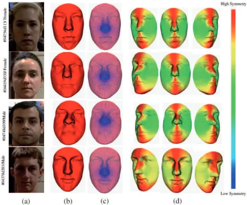
examples illustrating this symmetry descriptor are shown in Figure 2. For
214
each subject, face in column (a) shows the 2D intensity image; column (b)
215
illustrates the preprocessed 3D face surface S; column (c) illustrates the the
216
3D face S with extracted curves; column (d) shows the symmetry degree as
217
a color-map of the DSF mapped on S. The color bar is shown in the
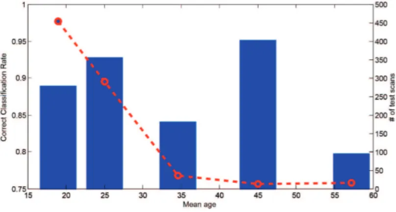
up-218
right corner. The hot colors mean the minimum difference (i.e. maximum
219
symmetry) and cold colors signify the maximum difference (i.e. minimum
Figure 2: Illustrations of the symmetry DSFs on faces. (a) 2D intensity image; (b) preprocessed 3D face S; (c) 3D face S with extracted curves; (d) color-map of symmetry DSF mapped on S with three poses. While the cold colors reflect lower symmetrical regions, the warm colors represent higher symmetrical parts of the face.
symmetry). The hotter the color, the higher is magnitude of the bilateral
221
symmetry. In this work, the symmetry DSFs are generated with 200 radial
222
curves extracted from each face and 100 indexed points on each curve. Thus,
223
the size of each DSF is 20000. The average time consumed for extracting
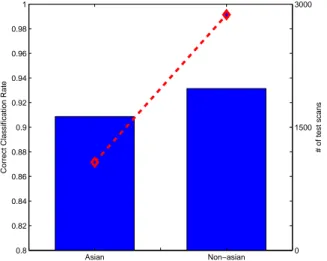
224
all 200 curves for each face is 1.048 seconds, and for generating the bilateral
225
symmetry descriptor (symmetry DSF) on all the 200 × 100 points of each
226
face is 0.058 seconds. The average preprocessing time consumed for each
Source face
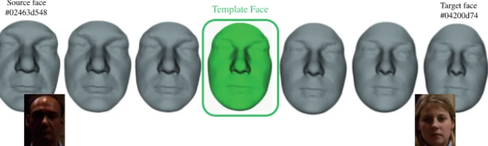
#02463d548 Template Face Target face#04200d74
Figure 3: The averageness face template is defined as the middle point of the geodesic path between two representative faces randomly taken from the male and female classes in the FRGCv2 dataset.
scan is 0.116 seconds. The total computation time (including preprocessing)
228
for each scan is less than 1.25 seconds. All our programs are developed in
229
C++ and executed on Intel Core i5 CPU 2.53 GHZ with 4Go of RAM.
230
2.3. Face averageness description
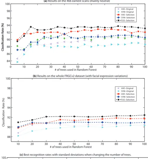
231
As mentioned earlier, generally, male faces have more prominent features
232
(forehead, eyebrows, nose, mouth, etc.) in comparison with female faces.
233
Here, our aim is to capture the morphologcial sexual differences between
234
male and female faces by comparing their shape differences to a defined face
235
template. We assume that such differences change with the face gender.
236
Thanks to DSF, presented in subsection 2.1, we are able to capture densely
237
such shape differences as long as a face template is defined.
238
As shown in Figure 3, the face template is defined as the middle point
239
of the geodesic path which connects a male face (ID: 02463d548; Age: 48;
240
White) to a female face (ID: 04200d74; Age: 21; White) taken from the
241
FRGCv2 dataset. With the two faces represented by collections of radial
242
curves, we compute pair-wisely the geodesic path between corresponding
curves using equation (1). By interpolation, we have the middle point of the
244
geodesic which we take as the face template T.
245
For a preprocessed face S, let βSα denote the radial curve that makes
246
an angle α with the middle plane PS(t, −→nh) from the frontal view of S, and
247
βT
α denotes the curve that makes the same angle α with PT(t, −→nh) in the
248
averageness face template T. The tangent vector field ˙ψα ∗
that represents the
249
projection of the deformation between the given face and the template face,
250
in the tangent space associated with the template face, is then calculated on
251
each point. Similar to the symmetry descriptor, with the magnitude of ˙ψα ∗
at
252
each point, located in curve βS
α with index k, we build an averageness Dense
253
Scalar Field (averageness DSF) on the facial surface, Vk
α = | ˙ψ∗α|(τ =0)(k)|. This
254
Dense Scalar Field quantifies the shape difference between corresponding
255
curves of S and T on each indexed point.
256
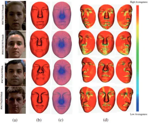
Figure 4 shows this averageness descriptor. For each subject, the face in
257
column (a) shows the 2D intensity image; column (b) illustrates the
prepro-258
cessed 3D face surface S; column (c) shows the 3D face S with extracted
259
curves; column (d) shows color-map of the Averageness DSF mapped on S
260
with three poses. The hot colors mean the minimum difference (i.e.
maxi-261
mum averageness) and cold colors signify the maximum difference (i.e.
min-262
imum averageness). The hotter the color, the higher is the magnitude of the
263
averageness.
264
3. Gender classification
265
In this work, face averageness and symmetry are different types of
infor-266
mation in the 3D facial shapes. Each of them provides a perspective (maybe
Figure 4: Illustrations of the averageness DSFs on faces. (a) 2D intensity image; (b) preprocessed 3D face surface S; (c) the 3D face S with extracted curves; (d) color-map of the Averageness DSF mapped on S with three poses. While the cold colors reflect lower averageness, the warm colors represent higher averageness on the face.
correlated perspectives) in face perception. Thus, we first study
individu-268
ally their relationship with gender, then we combine them to find out if it
269
enhances the gender classification results, which means that they contribute
270
to gender classification in different ways. In practice, we use an early fusion
271
method which consist in concatenating the averageness DSF and symmetry
272
DSF features of each scan, to form the fusion DSF description. Then, we
273
explore the performance of the Random Forest algorithm with the
geness DSF, the symmetry DSF and the fusion DSF in different scenarios,
275
in combination of Feature Selection methods. It has been demonstrated by
276
Perez et al. in [29], that different types of information (such as gray scale
277
intensity, range image and LBP texture) contributes to face based gender
278
classification differently, and the fusion of multi-information yields a better
279
classification performance.
280
3.1. Feature Selection
281
The size of the features is another important characteristic of the
ap-282
proach. As pointed out by Bekios-Calfa et al. in [28], in limited
computa-283
tional resource contexts, such as the mobiles, the development of
resource-284
limited algorithms is important for applications of computer vision and
pat-285
tern recognition. In their work, they make use of LDA techniques to reduce
286
feature size. In our work, we use feature selection methods to select a much
287
smaller set of the features to reduce the computational cost. Compared with
288
LDA techniques, feature selection methods do not tranferm the meaning and
289
values of feature, thus they allow to track back to the corresponding point
290
on the face.
291
Feature subset selection is the process of identifying and removing as
292
much irrelevant and redundant information as possible [22]. It is a central
293
problem in machine learning. The earliest approaches for feature selection
294
were the filter methods. These algorithms use heuristics based on general
295
characteristics of the data to evaluate the merit of feature subsets. Another
296
school of approaches argues that the bias of a particular induction algorithm
297
should be taken into account when selecting features. This method, called
298
the wrapper [23], uses an induction algorithm along with a statistical
sampling technique such as cross-validation to estimate the final accuracy of
300
feature subsets. The filter methods operate independently of any learning
301
algorithm. The undesirable features are filtered out of the data before the
302
learning begins. They are generally much faster than wrapper methods,
es-303
pecially on data of high dimensionality. Since the averageness, symmetry and
304
fusion DSFs are really dense and possibly redundant after DSF extraction, we
305
use a feature selection procedure on the DSFs to get rid of the irrelevant and
306
redundant features. For the merits of filter methods, we chose a filter, named
307
Correlation-based-Feature-Selection (CFS) [22]. It is an algorithm that
cou-308
ples the evaluation formula based on an appropriate correlation measure and
309
a heuristic search strategy. The central hypothesis of CFS is that good
fea-310
ture sets should contain features that are highly correlated with the class,
311
yet uncorrelated with each other. The feature evaluation formula (Pearsons
312
correlation coefficient), based on ideas from test theory, provides an
opera-313
tional definition of this hypothesis. Within CFS, we try two heuristic search
314
strategies, the Best-First search strategy and the Greedy-Step-Wise search
315
strategy. The Best-First search strategy [24] is an AI search strategy that
al-316
lows back-tracking along the search path. It moves through the search space
317
by greedy hill-climbing augmented with a back-tracking facility. When the
318
path being explored becomes non-improving, the Best-First search will
back-319
track to a more promising previous subset and continue the search from there.
320
The stopping criterion is the number of consecutive non-improving nodes (5
321
in our experiments) that result in no improvement. For Greedy-Step-Wise, it
322
performs a greedy forward or backward search through the space of attribute
323
subsets. It stops when the addition/deletion of any remaining attributes
results in a decrease in evaluation.
325
Selected Features for SYM (Symmetry)
(a) (b) (c) (d) (e) # 0 4 9 2 0 d 0 6 / F em al e # 0 4 2 3 7 d 1 5 3 /M al e High Symmetry Low Symmetry High Symmetry Low Symmetry High Averageness Low Averageness High Averageness Low Averageness
Selected Features for AVE (Averageness)
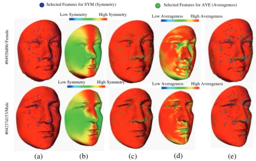
Figure 5: Feature selection. (a) selected points of symmetry DSF in the face; (b) color-map of original symmetry DSF; (c) selected points of averageness DSF in the face; (d) color-map of original averageness DSF; (e) selected points of both averageness DSF and symmetry DSF in face.
After Feature selection, we retain 301 salient points for averageness DSF,
326
271 salient points for symmetry DSF, and 365 salient points for the fusion.
327
The feature selection procedure significantly reduces the size and complexity
328
of original DSF description. Figure 5 shows the selected features of
aver-329
ageness DSF and symmetry DSF in faces. Column (a) maps the selected
330
features of symmetry DSF in the face; Column (b) shows the color-map of
331
original symmetry DSF on the face ; Column (c) maps the selected points
332
of averageness DSF in the face ; Column (d) shows the original averageness
333
DSF on the face; Column (e) maps the selected points of both averageness
334
DSF and symmetry DSF in the face. For both averageness DSF and
metry DSF, we observe dense distribution of salient points around the nose
336
and eyes regions. More salient points exist in forehead regions in
average-337
ness DSF, and more salient points exist in cheek regions in symmetry DSF.
338
These observations show that averageness DSF and symmetry DSF share
339
both similarities and differences. In other words, they are complementary in
340
face description.
341
3.2. Gender classification based on Random Forest
342
Face-based gender classification is a binary classification problem which
343
estimates the gender c of a given test face into Male or Female c ∈ {Male, F emale}.
344
We carry out gender classification experiments with the well-known machine
345
learning algorithm, Random Forest. Random Forest is an ensemble learning
346
method that grows many classification trees t ∈ {t1, .., tT} [25]. To classify a
347
new face from an input vector (DSF-based feature vector v = Vk
α), each tree
348
gives a classification result and the forest chooses the classification having
349
the most votes. In the growing of each tree, firstly, N instances are sampled
350
randomly with replacement from the original data, to make the training set.
351
Then, if each instance comprises of M input variables, a constant number m
352
(m<<M) is specified. At each node of the tree, m variables are randomly
353
selected out of the M and the best split on these m variables is used to split
354
the node. The process goes on until the tree grows to the largest possible
355
extent, without pruning.
356
The performance of the forest depends on the correlation between any
357
two trees, and the strength of each individual tree. The forest error rate
358
increases when the correlation decreases, or the strength increases. Reducing
359
m reduces both the correlation and the strength. Increasing it increases both.
Thus, an optimal m is needed for the trade-off between the correlation and
361
the strength. In Random Forest, the optimal value of m is found by using the
362
oob-error rate (out-of-bag-error rate). It is reported that face classification
363
by Random Forest achieves a lower error rate than some popular classifiers,
364
including SVM [20]. As far as we know, there is no reported work in the
365
literature of face-based gender classification using Random Forest.
366
4. Experiments
367
The FRGCv2 database was collected by researchers from the University
368
of Notre Dame [21] and contains 4007 3D face scans of 466 subjects with
369
differences in gender, ethnicity, age and expression. For gender, there are
370
1848 scans of 203 female subjects and 2159 scans of 265 male subjects. The
371
ages of subjects range from 18 to 70, with 92.5% in the 18 − 30 age group.
372
When considering ethnicity, there are 2554 scans of 319 White subjects,
373
1121 scans of 99 Asian subjects, 78 scans of 12 Asian-southern subjects, 16
374
scans of 1 Asian and Middle-east subject, 28 scans of 6 Black-or-African
375
American subjects, 113 scans of 13 Hispanic subjects, and 97 scans of 16
376
subjects subjects whose ethnicity are unknown. About 60% of the faces have
377
a neutral expression, and the others show expressions of disgust, happiness,
378
sadness and surprise. All the scans in FRGCv2 are near-frontal. With this
379
dataset, we conducted two experiments. The first one is to examine the
380
robustness of our approach to age and ethnicity variations. It uses the 466
381
earliest scan of each subject in FRGCv2, of which more than 93% are
neutral-382
frontal. The second one extends to examine the robustness of our approach
383
to variations of expression. It considers all the 4007 scans in FRGCv2, about
40% of which are expressive faces. For these experiments, the results are
385
generated in a subject-independent fashion, using a 10-fold cross-validation
386
setup.
387
4.1. Data preprocessing
388
The 3D face models present some imperfections, such as the holes (caused
389
by the absorption of the laser in the dark areas like eyebrows and eyes and
390
by the self-occlusions), the hair, and the spikes (caused by acquisition noise).
391
Thus, a preprocessing step is needed to limit their influence. Firstly, through
392
boundary detection, link-up and triangulation, holes are filled in each scan.
393
Secondly, since the scans in FRGCv2 are all near-frontal, the nose tip is
de-394
tected with a simple algorithm. The nose tip is detected by analyzing the
395
peak point of the face scan in the depth direction. Then, the mesh is cropped
396
with a sphere centered at the nose tip to discard the hair and the neck
re-397
gions. Finally, a smoothing filter is used to distribute evenly the 3D vertices
398
which capture the original 3D shape. We next perform the well-known
Iter-399
ative Closest Point (ICP) algorithm to normalize the poses of the obtained
400
meshes according to a reference mesh (frontal). The symmetry plane is then
401
picked up as the plane that has as origin the nose tip and has an horizontal
402
normal. In practice, the preprocessing step is performed automatically on
403
the whole FRGCv2 dataset without any manual intervention. We obtained
404
4005 well preprocessed scans after preprocessing. The failed two scans (with
405
scan id 04629d148 and 04815d208) were resulted from wrong nose tip
detec-406
tion. Considering the ratio of failure is rather tiny (2/4007<0.0005), we omit
407
the influence of the two failed scans for the results generation.
0 10 20 30 40 50 60 70 80 90 100 84 86 88 90 92 94 96 98 100
# of trees used in Random Forest
Classification Rate (%)Classification Rate (%)Classification Rate (%)
SYM−Original SYM−Selection AVE−Original AVE−Selection FUS−Original FUS−Selection 60 65 70 75 80 85 90 95 100 105
Best Classification Rate (%)
Earliest scans from FRGC−2.0 All scans from FRGC−2.0
(a) Results on the 466 earliest scans (mainly neutral)
(c) Best recognition rates with standard deviations when changing the number of trees.
10 20 30 40 50 60 70 80 90 100 88 90 92 94 96 98 100
# of trees used in Random Forest
Classification Rate (%) AVE−Original SYM−Original AVE−Selection SYM−Selection FUS−Selection (b) Results on the whole FRGCv2 dataset (with facial expression variations)
AVE−Original SYM−Original AVE−Selection SYM−Selection FUS−Selection
Figure 6: The reported results of the proposed methods1using Random Forest
4.2. Robustness to variations of age and ethnicity
409
Among the 466 earliest scans, 431 scans are neutral-frontal and 35 are
410
expressive-frontal. In our 10-fold cross validation setup, the 466 scans are
411
randomly partitioned into 10 folds with each fold containing 46 − 47 scans.
412
In each round, 9 of the 10 folds are used for training while the remaining
413
fold is used for testing. The average recognition rate and standard
devia-414
tion for 10 rounds then give a statistically significant performance measure.
415
The relationship between the gender classification result and the number of
416
trees used in the Random Forest is depicted in Figure 6(a). It demonstrates
417
that a significant relationship exists between gender and facial averageness
418
and facial symmetry considered separately. We note also that both the
fu-419
sion and the feature selection improve the gender classification results. In
420
fact, the fusion descriptor outperforms individual averageness and symmetry
421
descriptor. This implies that facial averageness and symmetry relate to
gen-422
der in different ways. At the same time, results after the feature selection
423
always override the results without feature selection. This means that the
424
original averageness DSF and symmetry DSF contain redundant information.
425
Gender-related features are distributed unequally in the facial regions. The
426
best gender classification rate is 93.78%, achieved by 80-Tree Random Forest
427
with the fusion descriptor after feature selection. This result is detailed in
428
the confusion matrix in Table 1. The recognition rate for females (92.02%) is
429
1Methods as described in Figure 1 : (1) the symmetry DSF features (SYM-Original),
(2) the selected features of symmetry DSF features (SYM-Selection), (3) the averageness DSF features Original), (4) the selected features of averageness DSF features (AVE-Selection), (5) the fusion of symmetry and averageness DSF features by concatenation (FUS-Original), and (6) the selected features of the fusion of symmetry and averageness DSF features (FUS-Selection).
slightly lower than for male ones (95.44%). It is probably due to the fact that
430
more male faces were used for training. We also performed a 10-fold
100-431
repetition experiment with Random Forest under the same setting, which
432
resulted at an average classification rate of 92.84% with a standard deviation
433
of 3.58%.
434
Table 1: Confusion matrix of RF-based classification.
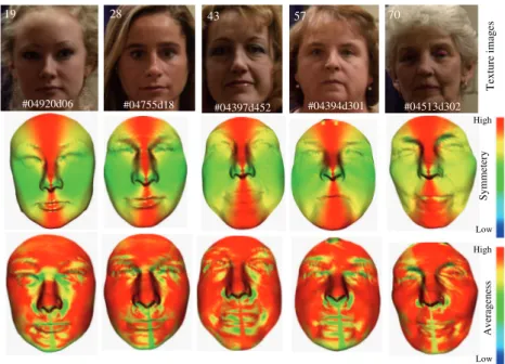
% Female Male Female 91.63 8.37 Male 4.56 95.44 Recognition Rate =93.78 ± 4.29% #04920d06 19 57 #04397d452 #04394d301 43 70 #04513d302 28 #04755d18 T ex tu re i m ag es Low High S y m m et er y A v er ag en es s Low High
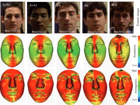
#04237d153 As-An #04428d241 As-As #04505d330 WH BA #04433d180 HI #04447d157 Low High S y m m et er y A v er ag en es s T ex tu re i m ag es Low High
Figure 8: DSFs on faces with different Ethnicity.
Figure 7 illustrates the color-maps of symmetry DSF and averageness
435
DSF on female faces with age differences and Figure 8 illustrates the
color-436
maps of symmetry DSF and averageness DSF on male faces with differences
437
in ethnicity. The information related to age, ethnicity and identity of scans
438
are presented in the 2D images in the upper row of each figure. Based on
439
the middle rows of Figure 7 and Figure 8, we can observe that the bilateral
440
symmetry of both genders convey a visually symmetrical pattern, where the
441
color-map of left-face is globally in symmetry with the right-face, although
442
subtle local asymmetry exists. Low-level deformations (red color) are usually
443
located near the middle plane and high-level deformations (yellow and green
444
colors) happen more frequently in further areas. The asymmetry, in female
445
faces, change obviously more smoothly than in male faces. On the other
hand, with the lower rows of Figure 7 and Figure 8, we observe that female
447
faces exhibit more deformations in mouth, nose and eye regions to deform
448
from the averageness face template. More subtly, in cheek and forehead
449
regions, the color is more consistent in male faces. All of these observations
450
above stay relatively consistent with changes of age and ethnicity. We believe
451
that these common patterns contribute to the robustness of our approach to
452
variations of age and ethnicity to some extent.
453
Figure 9: Gender classification results of different age group (the blue bars show the average recognition rate of each age group, and the red line shows the number of scans in this age group).
As it is well known that face perception is strongly affected by age [30],
454
we provide Figure 9 to analyze gender classification performance for different
455
age groups. In this figure, the blue bars show the average recognition rate for
456
each age group, and the red line shows the number of scans in the same age
457
group. We could confirm that gender classification is strongly influenced by
458
the age. Generally, although the gender classification results decrease from
459
above 90% to about 80% when increasing the age, all these results are near or
above 80%. That is to say the performance of our approach stays relatively
461
high with age variation. Moreover, due to unbalanced age distribution of
462
scans in FRGCv2 dataset, we see the number of scans decreased significantly
463
when the age is increased. We assume that this is also a reason for the
464
decrease of the gender classification results.
465 Asian Non−asian 0.8 0.82 0.84 0.86 0.88 0.9 0.92 0.94 0.96 0.98 1
Correct Classification Rate
0 1500 3000
# of test scans
Figure 10: Gender classification results of different ethnicity group (the blue bars show the average recognition rate of each age group, and the red line shows the number of scans in this ethnic group).
Figure 10 analyzes the relationship between the obtained classification
466
rate when varying the ethnicity. Here, the whole FRGCv2 dataset is
sepa-467
rated into Asian and Non-Asian groups. We can see that the gender
clas-468
sification rates, shown by the blue bars, stay above 90% when varying the
469
ethnicity. The classification rate of Non-Asian group is 3 − 4 percent higher
470
than that of the Asian group. This is probably due to a more sufficient
train-471
ing step has been involved with Non-Asian group, since it contains more than
two times of the number of the scans of the Asian group, as shown in the
473
figure by the red line.
474
4.3. Robustness to expression variations
475
In this experiment, with all the preprocessed scans of FRGCv2, we first
476
performed the DSF extraction for averageness, symmetry and fusion
descrip-477
tors, and then did the 10-fold subject-independent cross-validation with
Ran-478
dom Forest. For each round, the scans of 46 subjects are randomly selected
479
for testing, and the scans of the remaining subjects are dedicated to the
480
training. For all the 10 rounds of experiments, no common subjects are used
481
in training/testing. The relationship between the classification result and
482
the number of trees used in Random Forest is shown in Figure 6(b). We note
483
again that both fusion and feature selection improve the results. The best
484
result achieved with the fusion and feature selection is 92.46% ± 4.79 with
485
100-Tree Random Forest. We argue this result by the fact that the majority
486
of the selected features are located on the facial areas which are less affected
487
by the expressions in particular the nose, the eyebrows, and the forehead as
488
illustrated in Figure 5. Considering the FRGCv2 dataset is a challenging
489
dataset which contains as many as 4007 scans with various changes in age,
490
ethnicity and expression, we claim even more confident that a significant
re-491
lationship exists between gender and 3D facial averageness/symmetry, and
492
our method is effective and robust to ethnicity and expression variations.
#02463d550 #02463d552 #02463d556 #02463d558 #02463d562 T ex tu re i m ag es Low High S y m m et er y A v er ag en es s Low High
Figure 11: DSFs on faces with different expressions.
Figure 11 shows color-maps of DSFs generated for a subject with
differ-494
ent expressions. Similar to the observations in Figure 7 and Figure 8, we
495
perceive again in the middle row of Figure 11 that the symmetry
deforma-496
tions on both sides of the face are globally in symmetry, although tiny local
497
asymmetry exists in areas like eye corners and lips. Low-level deformations
498
(red) always locate near the middle plane and high-level deformations
(yel-499
low and green) occur more frequently in farther areas. With the lower rows
500
of Figure 7 and Figure 11, we observe again that female faces require more
501
deformation in mouth, nose and eye regions to deform from the averageness
502
face template. In cheek and forehead regions, the color is more consistent in
503
male faces. All these visible patterns do not change significantly with
expres-504
sion variations. We assume that these patterns contribute to the robustness
of our approach to expression changes. Figure 6(c) shows the best gender
506
recognition results (shown as bars) and their standard deviation (shown as
507
black lines) in our experiment. It shows that the gender recognition rate
508
increases with both fusion and feature selection, and the performances of all
509
the approaches change little between the 466 earliest scans protocol and the
510
whole FRGCv2 dataset protocol. It means our approach is even relatively
511
robust to the size of the training set.
512 0.7 0.75 0.8 0.85 0.9 0.95 1
Correct Classification Rate
Open mouth Closed mouth 0
2000 3500
# of test scans
Figure 12: Gender classification results of different expression group (the blue bars show the average recognition rate of each age group, and the red line shows the number of scans in this expression group).
Again, in Figure 12, we illustrate the effects of expression variations on
513
the proposed approach. We separated the FRGCv2 dataset into Open-mouth
514
and Closed-mouth groups. Despite the fact of the unbalanced number of
515
training scans in Open-mouth and Closed-mouth groups, as shown by the
516
red line, the results shown by the blue bars in the figure are all above 90%,
517
and the results between these two groups are comparable with each other.
4.4. Comparison with state of the art
519
Table 2 gives a comparison of this work with previous studies in 3D-based
520
gender classification. With differences in the dataset, landmarking,
exper-521
iment settings and so on, it is difficult to compare and rank these works
522
simply according to the result values. Compared with our work, works in [9],
523
[14], [15] are based on relatively smaller dataset which leave doubts about the
524
statistical significance of their performances on larger and more challenging
525
datasets. Works in [9], [12], [14], [15] require manual landmarking, thus they
526
are not fully-automatic. Works in [9], [14], [15], [16] use different
experi-527
mental settings other than the most prevailing 10-fold cross-validation. Our
528
work addressed gender classification in a fully automatic way without
man-529
ual landmarking. Experimented on a large dataset, FRGCv2, which contains
530
challenging variations in expression, age and ethnicity, and reached
competi-531
tive results with literature. The nearest works to ours are done by Ballihi et
532
al. in [17] and Toderici et al. in [3]. With the 466 Earliest scans of FRGCv2
533
and standard 10-fold cross-validation, Ballihi et al. achieved 86.05%
classifi-534
cation rate, while we achieved a much higher result of 93.78% by combining
535
facial shape averageness and bilateral asymmetry. In [3], Toderici et al. also
536
performed automatic 10-fold cross-validation on the FRGCv2 dataset in a
537
subject-independent fashion. In general, we have achieved comparable
re-538
sults than them. They achieve about 1% higher gender classification rate
539
than us. While we achieve a lower standard deviation which signifies better
540
stability of the algorithm than theirs2.
541
2During the work, we found 8 scans of a subject (id 04662, female indeed) had been
Table 2: Comparison of our approach to earlier studies. Reference Dataset Auto Features Classifiers Experiment
settings Results Shape/ Texture Ballihi et al. [17] 466 earli-est scans of FRGCv2
Yes facial curves Adaboost 10-fold cross-validation 86.05% Shape Toderici et al. [3] All scans of FRGCv2
Yes Wavelets Polynomial-SVM 10-fold cross-validation Male : 94 ± 5% Female : 93 ± 4% Shape Hu et al. [16] 729 UND scans and 216 private scans Yes Curvature based shape index RBF-SVM 5-fold cross-validation 94.03% Shape Han et al. [14] 61 3D scans in GavabDB No Geometry Features RBF-SVM 5-fold cross-validation 82.56 ± 0.92% Shape Wu et al. [15] Needle maps of 260 sub-jects from UND
No PGA features Posterior Probability 200 train/60 test, 6 repeti-tions 93.6 ± 4% Shape+ Texture Lu et al. [12] 1240 scans from UND and MSU No Grid element values Posterior Probability 10-fold cross-validation 91 ± 3% Shape+ Texture Liu et al. [9] 111 full 3D scans of 111 subjects No Variance Ra-tio in HD and OD faces linear clas-sifier half train/ half test, 100 repetitions HD:91.16 ± 3.15% OD:96.22 ± 2.30% Shape Our work1 466 earli-est scans of FRGCv2 Yes AVE+SYM DSFs Random Forest 10-fold cross-validation 93.78 ± 4.29% Shape Our work2 All scans of FRGCv2 Yes AVE+SYM DSFs Random Forest 10-fold cross-validation 92.46 ± 3.58% Shape 5. Conclusion 542
In this paper, we have proposed a fully automatic approach based on 3D
543
facial averageness/symmetry differences for gender classification. We have
544
proposed to use our Dense Scalar Fields grounding on Riemannian
Geom-545
etry to capture densely facial averageness and its bilateral symmetry. The
546
remaining challenge is the large dimensionality of the DSFs, which is handled
547
using a feature-selection-based dimension reduction, followed by a Random
548
Forest classifier. Despite the wide range of age, ethnicity and facial
ex-549
pressions, our method achieves a gender classification result of 93.78% ±
550
4.29% with 466 earliest scans of subjects, and 92.46% ± 3.58 on the whole
FRGCv2 dataset. We have also demonstrated that a significant relationship
552
exists between the gender and these two high-level cues in face perception,
553
the face averageness and symmetry. Our approach is competitive with
state-554
of-the-art approaches. One of the limitations of the proposed approach is the
555
dependence on near-frontal pose of faces to compute the symmetry and the
556
averageness DSFs.
557
References
558
[1] A. Cellerino and D. Borghetti and F. Sartucci, ”Sex differences in face
559
gender recognition in humans”, Brain Research Bulletin, vol. 63, 2004,
560
pp. 443-449.
561
[2] V. Bruce and AM. Burton and E. Hanna and P. Healey and O. Mason
562
and A. Coombes and R. Fright and A. Linney, ”Sex discrimination: how
563
do we tell the difference between male and female faces?”, Perception,
564
vol. 22, 1993, pp. 131152..
565
[3] G. Toderici and S. O’Malley and G. Passalis and T. Theoharis and
566
I. Kakadiaris, ”Ethnicity- and Gender-based Subject Retrieval Using
567
3-D Face-Recognition Techniques”, International Journal of Computer
568
Vision, vol. 89, 2010, pp. 382-391.
569
[4] J. Ylioinas and A. Hadid and M. Pietikinen, ”Combining Contrast
In-570
formation and Local Binary Patterns for Gender Classification”, Image
571
Analysis, vol. 6688, 2011, pp. 676-686.
572
[5] E. Makinen and R. Raisamo, ”An experimental comparison of gender
classification methods”, Pattern Recognition Letters, vol. 29, 2008, pp.
574
1544-1556.
575
[6] W. Yang and C. Chen and K. Ricanek and C. Sun, Changyin, ”Gender
576
Classification via Global-Local Features fusion”, Biometric Recognition,
577
vol. 7098, 2011, pp. 214-220.
578
[7] C. Shan, ”Learning local binary patterns for gender classification on
579
real-world face images”, Pattern Recognition Letters, vol. 33, 2012, pp.
580
431-437.
581
[8] N. Kumar and A. Berg and P.N. Belhumeur and S. Nayar,
”Describ-582
able Visual Attributes for Face Verification and Image Search”, Pattern
583
Analysis and Machine Intelligence, vol. 33, 2008, pp. 1962 -1977.
584
[9] Y. Liu and J. Palmer, ”A quantified study of facial asymmetry in 3D
585
faces”, Analysis and Modeling of Faces and Gestures,2003, pp. 222-229.
586
[10] LG. Farkas and G. Cheung, ”Facial asymmetry in healthy North
Amer-587
ican Caucasians. An anthropometrical study”, Angle Orthod,vol. 51,
588
1981, pp. 70-77.
589
[11] A. Little and B. Jones and C. Waitt and B. Tiddeman and D. Feinberg
590
and D. Perrett and C. Apicella and F. Marlowe, ”symmetry Is Related to
591
Sexual Dimorphism in Faces: Data Across Culture and Species”, PLoS
592
ONE, vol. 3, 2008, pp. e2106 .
593
[12] X. Lu and H. Chen and A. Jain, ”Multimodal facial gender and
ethnic-594
ity identification”, Proceedings of the 2006 international conference on
595
Advances in Biometrics, 2006, pp. 554-561.
[13] ”The main differences between male and female faces”,
597
www.virtualffs.co.uk.
598
[14] X. Han and H. Ugail and I. Palmer, ”Gender Classification Based on 3D
599
Face Geometry Features Using SVM”, CyberWorlds,2009, pp. 114-118.
600
[15] J. Wu and W. A. P. Smith and E. R. Hancock, ”Gender Classification
601
using Shape from Shading”,International Conference on Image Analysis
602
and Recognition, 2007, pp. 499-508.
603
[16] Y. Hu and J. Yan and P. Shi, ”A fusion-based method for 3D facial
gen-604
der classification”, Computer and Automation Engineering (ICCAE),
605
vol. 5, 2010, pp. 369-372.
606
[17] L. Ballihi and B. Ben Amor and M. Daoudi and A. Srivastava and
607
D. Aboutajdine, ”Boosting 3D-Geometric Features for Efficient Face
608
Recognition and Gender Classification”, IEEE Transactions on
Infor-609
mation Forensics & Security, vol. 7, 2012, pp. 1766-1779.
610
[18] H. Drira and B. Ben Amor and M. Daoudi and A. Srivastava and S.
611
Berretti, ”3D Dynamic Expression Recognition based on a Novel
Defor-612
mation Vector Field and Random Forest”, 21st International Conference
613
on Pattern Recognition, 2012.
614
[19] A. Srivastava and E. Klassen and S. H. Joshi and I. H. Jermyn, ”Shape
615
Analysis of Elastic Curves in Euclidean Spaces”, Pattern Analysis and
616
Machine Intelligence, vol. 33, 2011, pp. 1415 -1428.
[20] A. Z. Kouzani and S. Nahavandi and K. Khoshmanesh, ”Face
classifi-618
cation by a random forest”, TENCON 2007-2007 IEEE Region 10
Con-619
ference, 2007, pp. 1-4.
620
[21] P. J. Phillips and P. J. Flynn and T. Scruggs and K. W. Bowyer and
621
J. Chang and K. Hoffman and J. Marques and J. Min and W. Worek,
622
”Overview of the face recognition grand challenge”, Computer Vision
623
and Pattern Recognition, vol. 1, 2005, pp. 947 - 954.
624
[22] Mark A. Hall, ”Correlation-based Feature Subset Selection for Machine
625
Learning”, PhD thesis, Department of Computer Science, University of
626
Waikato, 1999, chapter 3-4.
627
[23] R. Kohavi, ”Wrappers for Performance Enhancement and Oblivious
De-628
cision Graphs”. PhD thesis, Stanford University, 1995, chapter 4.
629
[24] E. Rich and K. Knight, ”Artificial Intelligence”, McGraw-Hill College,
630
1991.
631
[25] L. Breiman, ”Random Forests”, Machine Learning, vol. 45, 2001, pp
632
5-32.
633
[26] Lines PA, Lines RR, Lines CA., ”Profilmetrics and facial esthetics”. Am
634
J Orthod, 1978, 73:640-57.
635
[27] Bradley N. Lemke, ”Surgical Anatomy of the Face”. Arch Opthalmol,
636
1995, 113(8):982.
637
[28] Bekios-Calfa J, Buenaposada JM, Baumela L., ”Revisiting linear
criminant techniques in gender recognition”. IEEE Trans Pattern Anal
639
Mach Intell, 2011 Apr, 33(4):858-64.
640
[29] C. Perez, J. Tapia, P. Estvez, C. Held., ”Gender Classification From Face
641
Images Using Mutual Information and Feature Fusion”. International
642
Journal of Optomechatronics - INT J OPTOMECHATRONICS, 2012,
643
vol. 6, no. 1, pp. 92-119.
644
[30] Ferrario VF, Sforza C, Ciusa V, Dellavia C, Tartaglia GM, ”The effect
645
of sex and age on facial asymmetry in healthy subjects: a cross-sectional
646
study from adolescence to mid-adulthood”, J Oral Maxillofac Surg, 2001
647
Apr, 59(4):382-8.