HAL Id: hal-01166252
https://hal.inria.fr/hal-01166252
Submitted on 26 Jun 2015
HAL is a multi-disciplinary open access
archive for the deposit and dissemination of
sci-entific research documents, whether they are
pub-lished or not. The documents may come from
teaching and research institutions in France or
abroad, or from public or private research centers.
L’archive ouverte pluridisciplinaire HAL, est
destinée au dépôt et à la diffusion de documents
scientifiques de niveau recherche, publiés ou non,
émanant des établissements d’enseignement et de
recherche français ou étrangers, des laboratoires
publics ou privés.
Governing Energy Consumption in Hadoop through
CPU Frequency Scaling: an Analysis
Shadi Ibrahim, Tien-Dat Phan, Alexandra Carpen-Amarie, Houssem-Eddine
Chihoub, Diana Moise, Gabriel Antoniu
To cite this version:
Shadi Ibrahim, Tien-Dat Phan, Alexandra Carpen-Amarie, Houssem-Eddine Chihoub, Diana Moise, et
al.. Governing Energy Consumption in Hadoop through CPU Frequency Scaling: an Analysis. Future
Generation Computer Systems, Elsevier, 2016, pp.14. �10.1016/j.future.2015.01.005�. �hal-01166252�
Future Generation Computer Systems 00 (2015) 1–20
Governing Energy Consumption in Hadoop through CPU Frequency
Scaling: an Analysis
Shadi Ibrahim
a,∗, Tien-Dat Phan
b, Alexandra Carpen-Amarie
c, Houssem-Eddine
Chihoub
d, Diana Moise
e, Gabriel Antoniu
aaInria, Rennes Bretagne Atlantique Research Center, France bInria/IRISA Rennes, France
cVienna University of Technology, Austria dLIG, Grenoble Institute of Technology, France
eCray Inc., Switzerland
Abstract
With increasingly inexpensive storage and growing processing power, the cloud has rapidly become the environment of choice to store and analyze data for a variety of applications. Most large-scale data computations in the cloud heavily rely on the MapRe-duce paradigm and on its Hadoop implementation. Nevertheless, this exponential growth in popularity has significantly impacted power consumption in cloud infrastructures. In this paper, we focus on MapReduce processing and we investigate the impact of dynamically scaling the frequency of compute nodes on the performance and energy consumption of a Hadoop cluster. To this end, a series of experiments are conducted to explore the implications of Dynamic Voltage and Frequency Scaling (DVFS) settings on power consumption in Hadoop clusters. By enabling various existing DVFS governors (i.e., performance, powersave,
onde-mand, conservative and userspace) in a Hadoop cluster, we observe significant variation in performance and power consumption
across different applications: the different DVFS settings are only sub-optimal for several representative MapReduce applications. Furthermore, our results reveal that the current CPU governors do not exactly reflect their design goal and may even become inef-fective to manage the power consumption in Hadoop clusters. This study aims at providing a clearer understanding of the interplay between performance and power management in Hadoop clusters and therefore offers useful insight into designing power-aware techniques for Hadoop systems.
Keywords: MapReduce, Hadoop, power management, DVFS, governors
1. Introduction
Power consumption has started to severely constrain the design and the way data-centers are operated. Power bills became a substantial part of the monetary cost for data-center operators. Hamilton [1] estimated that the money spent on electrical power of servers and cooling units had exceeded 40 percent of the total expenses of data centers in 2008. The surging costs of operating large data-centers have been mitigated by the advent of cloud computing, which allowed for better resource management, facilitated by the adoption of virtualization technologies. Nevertheless,
∗Corresponding author.
Email address: [email protected] (Shadi Ibrahim) 1
overall energy consumption is continuously increasing as a result of the rapidly growing demand for computing resources. While various energy-saving mechanisms have been devised for large-scale infrastructures, not all of them are suitable in a cloud context, as they might impact the performance of the executed workloads. For instance, shutting down nodes to reduce power consumption may lead to aggressive virtual machine consolidation and resource over-provisioning, with dramatic effects on application performance.
Green cloud computing has thus emerged in an attempt to find a proper tradeoff between performance requirements and energy efficiency. To address this challenge, green clouds focus on optimizing energy-saving mechanisms at the level of the data-center through static and dynamic mapping of virtual machines (i.e., VMs) to physical resources or through efficient task consolidation [2, 3, 4, 5, 6]. For example, Xu and Fortes [4] propose a cross-layer control system to manage the dynamic mapping of VMs to physical resources. Two energy-conscious task consolidation heuristics are presented in [5] to maximize resource utilization while taking into account both active and idle energy consumption. To reduce the energy cost and carbon emission, some studies have focused on exploiting renewable energy sources in the cloud [7, 8]. GreenSlot [8] schedules the workloads to maximize the green energy consumption while meeting the jobs’ deadlines. To do so, it relies on an intelligent model to predict the amount of solar energy that will be available in the near future. Many research efforts have targeted power-saving techniques based on the Dynamic Voltage Frequency Scaling (DVFS) support in modern processors [9, 10]. In [9], a new scheduling algorithm is presented to allocate virtual machines in a DVFS-enabled cluster by dynamically scaling the supplied voltages. All these efforts share a global goal: to enable energy-efficient computation while still keeping performance at the required level.
In this paper, we shift focus from computation to data: we investigate the efficiency of such techniques in the context of large-scale data processing, which corresponds to an increasing share of today’s cloud applications. Today’s most popular paradigm for large-scale data processing, proposed by Google, is the MapReduce model [11], which gained a wide adoption due to features including scalability, fault tolerance, and simplicity. Its most well-known open-source implementation, Hadoop [12], was designed to process hundreds of terabytes of data on thousands of cores at Yahoo!. As such large-scale deployments became more and more common place on cloud infrastructures, enabling energy-efficient MapReduce processing becomes nowadays an essential concern in data centers. This started to motivate several studies on power saving in Hadoop clusters [13, 14].
MapReduce systems span over a multitude of computing nodes that are frequency- and voltage-scalable. Further-more, many MapReduce applications show significant variation in CPU load during their running time. Moreover, MapReduce applications range from CPU-Intensive to I/O-Intensive, a typical MapReduce application comprising many subtasks, such that the workload of each subtask is either CPU-bound, I/O-bound or network-bound. Thus, there is a significant potential for saving energy by scaling down the CPU frequency when the currently executed task does not fully utilize the available computational resources.
The contribution of this paper is to investigate such opportunities for optimizing energy consumption in Hadoop clusters. We rely on a series of experiments to explore the implications of DVFS settings on power consumption in Hadoop clusters. As DVFS research has reached a certain maturity, several CPU Frequency Scaling tools and
governors have been proposed and implemented in the Linux kernel. A governor is a power scheme that can drive CPU
core frequency/voltage operation based on a specific policy, using a specific kernel module. For instance, governors such as ondemand or performance tune the CPU frequency to optimize application execution time, while powersave is designed to lower energy consumption.
We study the impact of different governors on Hadoop’s performance and power efficiency. Interestingly, our experimental results report not only a noticeable variation of the power consumption and performance with different applications and under different governors, but also demonstrate the opportunity to achieve a better tradeoff between performance and power consumption.
The primary contributions of this paper are as follows:
1. It provides an overview of the state-of-the-art techniques for energy-efficiency in Hadoop.
2. It discusses and demonstrates the need for exploiting DVFS techniques for energy reduction in Hadoop. 3. It experimentally demonstrates that MapReduce applications experience variations in performance and power
consumption under different CPU frequencies (similarly to [15]) and also under different governors. A micro-analysis section is provided to explain this variation and its cause.
4. It illustrates in practice how the behavior of different governors influences the execution of MapReduce appli-cations and how it shapes the performance of the entire cluster.
5. It also brings out the differences between these governors and CPU frequencies and shows that they are not only sub-optimal for different applications but also sub-optimal for different stages of MapReduce execution. 6. It demonstrates that achieving better energy efficiency in Hadoop cannot be done simply by tuning the
gover-nor parameters, gover-nor through a na¨ıve coarse-grained tuning of the CPU frequencies [15, 16] or the govergover-nors according to the running phase (i.e., map phase or reduce phase).
Overall, this study aims to provide a clearer understanding of the interplay between performance and power management in Hadoop clusters, with the purpose of deriving useful insights for designing power-aware techniques for Hadoop.
Relationship to previous work. This paper extends our previous contribution introduced in [17] (as a chapter in [18])
by providing more detailed descriptions and more thorough experiments. In particular, we provide more details to clearly illustrate our motivation in this work (i.e., the motivation for investigating DVFS in Hadoop). We include more experiments to illustrate the behavior of different governors, which influence the energy consumption in Hadoop MapReduce. We extend our experimental platform from 15 to 40 nodes and we employ two more benchmarks:
K-means and wordcount. The major extension of our previous work lies in the fact that in this paper we take a step
further in achieving energy efficiency tailored for Hadoop applications. While our previous work shows the potential for reducing energy consumption by tuning CPU frequencies and governor policies, in this work we explore that potential and investigate preliminary DVFS models that adjust to the various stages of Hadoop applications. We also demonstrate that achieving better energy efficiency in Hadoop cannot be done by tuning the governor parameters, nor through a na¨ıve coarse-grained tuning of the CPU frequencies or the governors according to the running phase (i.e., map phase or reduce phase). Moreover, we provide an extensive discussion on the application behavior sensitivity to different parameters employed in ondemand and conservative governors.
Paper Organization. The rest of this paper is organized as follows: Section 2 briefly presents Hadoop and how it
copes with existing CPU power-management techniques. This section also discusses our motivation and the related work. Section 3 provides an overview of our methodologies, followed by the experimental results in Sections 4 and 5. Section 6 discusses the implications of the fixed, configurable, and dynamic policies on the energy efficiency in Hadoop. Finally, we conclude the paper and discuss our future directions in Section 7.
2. Background, motivation and related work
In this section, we briefly introduce Hadoop and existing DVFS mechanisms. This section also presents related work on MapReduce energy consumption in data-centers and clouds.
2.1. Hadoop
Yahoo!’s Hadoop project [12] is a collection of various sub-projects for supporting scalable and reliable distributed computing. The two fundamental sub-projects feature a distributed file system (HDFS) and a Java-based open-source implementation of MapReduce through the Hadoop MapReduce framework. HDFS is a distributed file system that relies on a master/slave architecture to provide high-throughput access to application data [12]. The master server, called NameNode, splits files into chunks and distributes them across the cluster with replication for fault tolerance. It holds all metadata information about stored files. The HDFS slaves are called DataNodes and are designed to store data chunks, to serve read/write requests from clients and propagate replication tasks as directed by the NameNode. Hadoop MapReduce is a software framework for distributed processing of large data sets on compute clusters. It runs on top of HDFS, thus collocating data storage with data processing. A centralized JobTracker (JT) is responsible for: (a) querying the NameNode for the block locations, (b) scheduling the tasks on TaskTrackers (TT), based on the information retrieved from the NameNode, and (c) monitoring the success and failures of the tasks.
CpuFreq Governor
Goal Short description Downsides
Performance Maximize Performance Statically sets the CPU frequency to the highest
available frequency
High power consumption
Powersave Maximize power savings Statically sets the CPU frequency to the lowest
available frequency
Long response time
Ondemand Power efficiency with
reasonable performance
Dynamically adjusts the CPU frequency to the highest available frequency when the load is high and gradually degrades the CPU frequency when the load is low
Low performance/power
saving benefits when the
system switches between
idle states and heavy load often
Conservative Power efficiency with
reasonable performance
Gradually upgrades the CPU frequency when the load is high and gradually degrades the CPU fre-quency when the load is low
Worse performance than
Ondemand
Userspace Support for user-defined
frequencies
Statically sets the CPU frequency to a user-defined value
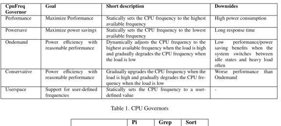
-Table 1. CPU Governors
Pi Grep Sort Average CPU-usage 70.11% 64.74% 23.05%
Table 2. Average CPU Usage for the three MapReduce applications
2.2. Power Management at CPU Level
Modern processors offer the ability to tune the power mode of the CPU through the introduction of idle processor operating states (C-states) and CPU performance states (P-states). A C-state indicates whether the processor is cur-rently active or not: processors in C0state are executing instructions while processors in higher C-states (Ci where
i= 1, 2, etc.) are considered idle. Higher C-states reflect a deeper sleep mode, and thus increased power savings.
P-states determine the processor frequencies and their associated voltage: Processors in the P0 state run at the
highest frequency and processors in the highest P-state run at the lowest frequency. The number of available P-states varies depending on the processor type.
Dynamic Voltage and Frequency Scaling (DVFS) is a commonly used technique that improves CPU utilization and power management by tuning the CPU frequency according to the current load. The ideal DVFS mechanism can instantaneously change the voltage/frequency values. Since the 2.6.10 version of the Linux kernel, there are five different power schemes (governors) available to dynamically scale the CPU frequency according to the CPU utilization. Each governor which favors either performance or power efficiency, as shown in Table 1. More details can be found in [19]). Moreover, setting the governor to userspace allows users to adjust the CPU frequency to a fixed value among the ones supported by the processors. Additionally, modern CPUs provide a new feature called Turbo Boost, which enhances the performance of a subset of a machine’s cores by boosting their clock speed, while the rest of the available cores are in a sleep state.
2.3. Why DVFS in Hadoop?
We explore two orthogonal dimensions that motivate the need for fine-tuning CPU performance and, consequently, energy consumption in Hadoop clusters.
2.3.1. Diversity of MapReduce applications
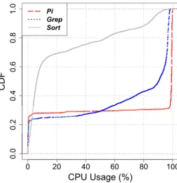
The wide adoption of Hadoop MapReduce results in a huge proliferation of MapReduce applications including scientific applications: astronomy, genomics, machine learning, graph analysis, and so on. These applications have different characteristics and therefore vary in their resource usage (i.e., CPU power usage). Our study, conducted on a Grid’5000 cluster [20], investigates the CPU-usage variation for three representative MapReduce benchmarks (Pi, Grep and Sort). As shown in Table 2, the average CPU usage significantly differs according to the running applications: the average CPU usage is 70.11% and 64.74% for the pi and grep applications, while it is only 23.05% for sort application. Moreover, as shown in Figure 1, the CPU load is high (more than 90%) during almost 75% of the job running time for the Pi application and is relatively high (more than 75%) only during 65% and 15% of the job running time for Grep and Sort jobs, respectively.
0 20 40 60 80 100 0 .0 0 .2 0 .4 0 .6 0 .8 1 .0 CPU Usage (%) C D F Pi Grep Sort
Figure 1. CPU utilization when running Pi, Grep and Sort benchmarks with 7.5GB of data in a 15-node Hadoop cluster: for the Pi and
Grep applications, which represent CPU-intensive MapReduce applications, we observe that the CPU load is either high - more than 90% and 80%
during 75% and 55% of the job running time - or low - less than 1% for 21% of the job running time, respectively. Conversely, for Sort, a mostly I/O-intensive application, the CPU load has more variation.
2.3.2. Multi-phase MapReduce’s job execution
By design, each MapReduce job is divided into two phases: map and reduce. As shown in Figure 2, a map task starts by reading the input records, then it applies the map function and outputs key-value pairs of intermediate data. Intermediate key-value pairs are partitioned, sorted and spilled to the local disk into separated indexed files. The reduce tasks start as soon as the intermediate indexed files are written to the local disk. The files from multiple local map outputs are written at the same time and then they are buffered in memory in a “shuffle buffer” and saved on the local disk. Finally the merged data are passed to the reduce function and then the output is written back to HDFS.
Using static program analysis, we can identify the access pattern of a MapReduce application, according to the amount of work per subtask. Thus, as each subtask workload relies either on computation, or on disk requests or bandwidth requests, we can easily reduce the space of profiled options into the resource utilization space, as shown in Figure 2:
• Disk I/O-intensive. From the application start to the moment the first map input is read into memory. • Computation. From the time the first map input is read to the first map output spilled to disk.
• Computation, disk and network I/O-intensive. From the moment the first map is spilled to disk until all maps are done.
• Disk and network I/O-intensive. Starts when all maps are done and lasts until the shuffle phase is done. • Computation and disk I/O-intensive. From the end of the shuffle phase until all reducers are done. • Disk I/O-intensive. Starts when all reducers are done and ends when the job is completely finished.
The length of each phase is highly dependent on the number of maps that are expected to be executed on each node, on the size of intermediate data, and on the number of reducers that are expected to be executed on each node. Moreover, the CPU load during each phase is determined by the complexity of the map and reduce functions defined in the applications.
As a consequence, there is a significant potential for reducing energy consumption by scaling down the CPU frequency when the peak CPU performance is not required by the workload or by the MapReduce phase.
Figure 2. Workflow of the two phases of MapReduce, Map phase and Reduce phase
2.4. Related Work
MapReduce has attracted much attention in the past few years [21]. Substantial research efforts have been ded-icated to either adopting MapReduce in different environments such as multi-core [22], graphics processors (GPUs) [23], and virtual machines [24, 25] or to improving MapReduce performance through skew-handling [26, 27], locality-execution [28, 29], and disk I/O scheduling [30, 31].
There have been several studies on evaluating and improving the MapReduce energy consumption in data-centers and clouds. Many of these studies focus on power-aware data-layout techniques [32, 33, 34, 35, 36, 37], which allow servers to be turned off without affecting data availability. GreenHDFS [33] separates the HDFS cluster into hot and cold zones and places the new or high-access data in the hot zone. Servers in the cold zone are transitioned to the power-saving mode and data are not replicated, thus only the server hosting the data will be woken up upon future access. Rabbit [32] is an energy-efficient distributed file system that maintains a primary replica on a small subset of always on nodes (active nodes). Remaining replicas are stored on a larger set of secondary nodes which are activated to scale up the performance or to tolerate primary failures. These data placement efforts could be combined with our approach to reduce the power consumption of powered servers. Instead of covering a set of nodes, Lang and Patel propose an all-in strategy (AIS) [38]. AIS saves energy in an all-or-nothing fashion: the entire MapReduce cluster is either on or off. All MapReduce jobs are queued until a certain threshold is reached and then all the jobs are executed with full cluster utilization.
Some works consider energy saving for MapReduce in the cloud [13, 39]. Cardosa et al. [13] present virtual machine (VM) replacement algorithms that co-allocate VMs with similar runtime to the same physical machine in a way that increases the utilization of available resources. Consequently, this maximizes the number of idle servers that can be deactivated to save energy. Chen et al. [40] analyze how MapReduce parameters affect energy efficiency and discuss the computation versus I/O tradeoffs when using data compression in MapReduce clusters in terms of energy efficiency [14]. Chen et al. [41] present the Berkeley Energy Efficient MapReduce (BEEMR), an energy efficient MapReduce workload manager motivated by empirical analysis of real-life MapReduce with Interactive Analysis (MIA) traces at Facebook. They show that interactive jobs operate on just a small fraction of the data, and thus can be served by a small pool of dedicated machines with full power, while the less time-sensitive jobs can run in a batch fashion on the rest of the cluster. Recently, Mashayekhy et al. [42] designed a framework for improving the energy efficiency of MapReduce applications, while satisfying the service level agreement (SLA). The proposed framework relies on a greedy algorithm to find the assignments of map and reduce tasks to the machine slots in order to minimize the energy consumed when executing the application. Goiri et al. [7] present GreenHadoop, a MapReduce framework for a data-center powered by renewable green sources of energy (e.g. solar or wind) and the electrical grid (as a backup). GreenHadoop schedules MapReduce jobs when green energy is available and only uses brown energy to avoid time violations.
Many existing studies focus on achieving power efficiency in Hadoop clusters by using DVFS [16, 15]. Li et 6
Figure 3. An overview of techniques to improve energy efficiency in Hadoop
al. [16] discuss the implications of temperature (i.e., machine heat) on performance and energy tradeoffs of MapRe-duce. Based on the observation that higher temperature causes higher power consumption even with the same DVFS settings, they propose a temperature-aware power allocation (TAPA) that adjusts the CPU frequencies according to their temperature. TAPA favors the maximum possible CPU frequency, thus maximizing computation capacity, with-out violating the power budget. Wirtz and Ge [15] compare the power consumption and the performance of Hadoop applications in three settings: (1) fixed frequencies, (2) setting the frequencies to maximum frequencies when execut-ing the map or reduce, and minimum otherwise, and (3) performance-constraint frequency settexecut-ings that tolerate some performance degradation while achieving better power consumption. Our work relies on “Fine-grained” frequen-cies and governors assignment, aiming to achieve the same performance, while minimizing the power consumption. Figure 3 summarizes existing techniques to improve energy efficiency in Hadoop.
Dynamic Voltage and Frequency Scaling Techniques. There is a large body of work on techniques that control the DVFS mechanisms for power-scalable clusters [43, 44, 45, 46, 47]. Some of these techniques control the CPU frequencies at runtime [45] and some scale the frequencies statically, based on extensive and expensive application profiling [43]. However, our approach differs from such works, as we target a different type of applications, namely MapReduce applications.
3. Methodology Overview
The experimental investigation conducted in this paper focuses on exploring the implications of executing MapRe-duce applications under different DVFS settings. We conducted a series of experiments in order to assess the impact of various DVFS configurations on both power consumption and application performance.
3.1. Platform
The experiments were carried out on the Grid’5000 [20] testbed. The Grid’5000 project provides the research community with a highly-configurable infrastructure that enables users to perform experiments at large scales. The platform is spread over 10 geographical sites located in France. For our experiments, we employed nodes belonging to the Nancy site of Grid’5000. These nodes are outfitted with 4-core Intel 2.53 GHz CPUs and 16 GB of RAM. Intra-cluster communication is done through a 1 Gbps Ethernet network. It is worth mentioning that only 40 nodes of the Nancy site are equipped with power monitoring hardware, consisting of 2 Power Distribution Units (PDUs), each hosting 20 outlets. Since each node is mapped to a specific outlet, we are able to acquire coarse and fine-grained power monitoring information using the Simple Network Management Protocol (SNMP). It is important to state that Grid’5000 allows us to create an isolated environment in order to have full control over the experiments and the obtained results.
3.2. Benchmarks
MapReduce applications are typically categorized as CPU-intensive, I/O bound, or both. For our analysis, we selected three applications that are commonly used for benchmarking MapReduce frameworks: distributed grep,
distributed sort and distributed pi.
• Distributed grep. This application scans the input data in order to find the lines that match a specific pattern. The grep example can be easily expressed with MapReduce: the map function processes the input file line by line and matches each single line against the given pattern; if the matching is successful, then the line is emitted as intermediate data. The reduce function simply passes the intermediate data as final result.
• Distributed sort. The sort application consists in sorting key/value records based on their key. With MapRe-duce, both the map and reduce functions are trivial computations, as they simply take the input data and emit it as output data. The sort MapReduce implementation takes advantage of the default optimizations performed by the framework that implicitly sorts both intermediate data and output data.
• Distributed pi. This benchmark estimates the value of pi based on sampling. The estimator first generates random points in a 1×1 area. The map phase checks whether each pair falls inside a 1-diameter circle; the reduce phase computes the ratio between the number of points inside the circle and the ones outside the circle. This ratio gives an estimate for the value of Pi.
Out of these three benchmarks, pi is purely CPU-intensive, while grep and sort are also I/O bound. However, sort is more data-intensive than grep, since it generates significantly more output data.
3.3. Hadoop deployment
On the testbed described in Section 3.1, we configured and deployed a Hadoop cluster using the Hadoop 1.0.4 stable version [12]. The Hadoop instance consists of the NameNode, the JobTracker and the Hadoop client, each deployed on a dedicated machine, leaving 13 nodes to serve as both DataNodes and TaskTrackers. The TaskTrackers were configured with 4 slots for running map tasks and 2 slots for executing reduce tasks. At the level of HDFS, we used the default chunk size of 64 MB and the default replication factor of 3 for the input and output data. In addition to facilitating the tolerance of faults, data replication favors local execution of mappers and minimizes the number of remote map executions. Prior to running the benchmarks, we generated 900 chunks of text (adding up to 56 GB) to feed the grep and sort applications. This input size results in fairly long execution times, which allowed us to thoroughly monitor power consumption information.
3.4. Dynamic Voltage Frequencies settings
The experiments we conducted involve running the benchmarks with various CPU settings and monitoring the power consumed by each node in this time frame. We distinguish a total of 15 scenarios corresponding to various val-ues for CPU governors and frequencies. We varied the used governor between conservative, ondemand, performance,
powersave, and userspace. With the governor set to userspace, we tuned the CPU frequency to each of the
follow-ing available values: 1.2 GHz, 1.33 GHz, 1.47 GHz, 1.6 GHz, 1.73 GHz, 1.87 GHz, 2 GHz, 2.13 GHz, 2.27 GHz, 2.4 GHz, 2.53 GHz.
4. Macroscopic Analysis
In this section, we provide a high-level analysis of the experimental results we obtained. Our goal is to study the impact of various governors or CPU frequencies on the performance of several classes of MapReduce applications.
Figure 4 depicts the completion time and the energy consumption of each governor for our three applications:
pi, grep and sort. Each point on the graphs stands for the application runtime and the total energy consumption of
the Hadoop cluster during its execution for a specific CPU frequency or governor. We computed the total energy consumption for each application as the sum of the measured utilized power of each cluster node with a resolution of 1 second between measurements. In addition, Figure 5 displays a comparative view of the average power consumption of a job for each of the three applications and DVFS settings.
200 300 400 500 600 35000 0 45000 0 5 50000 Response Time (s) Energy (Joule) 2.4GHz 2.0GHz 2.13GHzPerformance 1.87GHz OnDemand Conservative 2.27GHz 2.53GHz 1.6GHz 1.73GHz 1.47GHz 1.33GHz 1.2GHz Powersave (a) Pi 200 250 300 350 400 500 34000 0 380 000 420000 Response Time (s) Energy (Joule) 2.27GHz 2.53GHz 2.0GHz 1.87GHz 2.4GHz OnDemand 2.13GHz Conservative Performance1.73GHz 1.6GHz 1.47GHz 1.33GHz 1.2GHz Powersave (b) Grep 600 650 700 750 800 850 950 70000 0 80000 0 9 00000 Response Time (s) Energy (Joule) 2.0GHz Conservative 1.47GHz 2.53GHz 1.87GHz 2.27GHz OnDemand Powersave 1.33GHz 1.73GHz Performance 2.13GHz 1.6GHz 2.4GHz 1.2GHz (c) Sort
Figure 4. Application runtime vs Energy consumption under various DVFS settings
Pow ersa ve 1.2GHz1.33GHz1.47GHz1.6GHz1.73GHz1.87GHz2.0GHz2.13GHz2.27GHz2.4GHz2.53GHz Per form ance Conse rvative OnDe man d 20 40 60 80 100 120 P ow er ( W a tt) (a) Pi Pow ersa ve 1.2GHz1.33GHz1.47GHz1.6GHz1.73GHz1.87GHz2.0GHz2.13GHz2.27GHz2.4GHz2.53GHz Per form ance Conse rvative OnDe man d 20 40 60 80 100 120 P ow er ( W a tt) (b) Grep Pow ersa ve 1.2GHz1.33GHz1.47GHz1.6GHz1.73GHz1.87GHz2.0GHz2.13GHz2.27GHz2.4GHz2.53GHz Per form ance Conse rvative OnDe man d 20 40 60 80 100 120 P ow er ( W a tt) (c) Sort
Figure 5. Average Power consumption under various DVFS settings
4.1. Performance analysis
As expected, the results show the job completion time increases as the employed CPU frequency decreases, for each of the three applications. However, this does not happen at the same extent for all applications. In the case of the pi and grep applications, the runtime increases by 104% and 70%, respectively, when replacing the highest frequency, that is 2.53 GHz, with the lowest one, namely 1.2 GHz. The explanation for this behavior comes from the fact that the runtime of these two applications mostly accounts for computation, as they produce very little output data. Thus, the CPU performance has a significant impact on application execution time. The sort application is I/O-bound, generating the same amount of output data as the input data. As in our experiments we employed an input file of 900 chunks replicated 3 times, i.e. 56 GB of processed data and 168 GB of output data, sort spent a significant percentage of its execution time in reading data from and writing it to HDFS. Consequently, unlike pi and grep, the
sort application exhibits a different behavior: reducing the CPU frequency from the highest to the lowest possible
value only results in a 38% runtime increase.
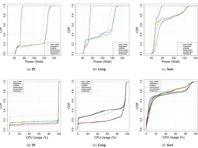
These results are consistent with the CDF of the CPU usage depicted in Figure 6. Pi is a purely CPU-intensive application and consequently its CPU usage is the highest, amounting over 80% for most of the CPU frequencies and governors. At the other end of the spectrum, the I/O-bound workload of sort is the main factor that accounts for an average CPU usage between 20% and 28%.
4.2. Energy consumption
The energy consumption on a Hadoop cluster depends on several parameters. One key factor is the CPU fre-quency, as low CPU frequencies also trigger low power consumption for a specific node. The application workload can however have an essential influence on the total energy utilized by the cluster. On the one hand, CPU-bound applications account for high CPU usage and thus for an increased energy consumption. Additionally, the application runtime directly impacts the energy needed by the cluster, and thus, attempts to improve application performance may result in better energy efficiency. In this section we analyze the tradeoff between the aforementioned factors in the case of our three types of applications.
Figure 5(a) details the average power consumption of a cluster node for each of the available fixed frequencies and all the governors, computed over the execution time of each application and the averaged across all cluster nodes. The average power consumption of a cluster node for pi is significantly lower for inferior CPU frequencies, as well as for the powersave governor. This observation would typically translate into an efficient total energy consumption at the level of the cluster for low frequencies. However, as Figure 4(a) demonstrates, the highest CPU frequency, that is 2.53 GHz, achieves the best results both in terms of performance and energy-efficiency. This behavior can be explained by analyzing the workload: pi is a CPU-intensive application, which can achieve 104% better performance by employing the highest CPU frequency, as shown in Section 4.1, whereas the average power consumption only increases by 48%. The same trend can be noticed for the grep and sort applications. Nevertheless, the energy savings induced by using the highest available frequency proportionally decrease with the percentage of CPU usage of the application. Thus, as sort uses the least amount of CPU power, its runtime is not significantly impacted by reducing the CPU frequency and the total energy consumption of the application only increases by 15% between the highest and lowest CPU frequency values. The average power consumption for sort displayed in Figure 5(c) confirms this behavior, as the low CPU utilization at high CPU frequencies such as 2.53 GHz leads to only a 22% increase of the consumed power per node.
Discussion. We can conclude that the workload properties play an essential role in establishing the
energy-consumption profile of an application. When the application runtime predominantly accounts for CPU usage, the most power-consuming CPU settings can surprisingly trigger a better total energy efficiency. Accordingly, applications that feature both I/O- and CPU-intensive phases, can benefit from adaptive CPU frequency policies by maximizing the CPU performance only during the computation stages of the application. Such policies can ensure a reduced energy consumption at the level of the application in two steps. First, for the CPU-intensive phases the total energy can be decreased by reducing the execution time, as it is the case for Pi. Second, the duration of the I/O-bound phases is not dependent of the CPU frequency settings and therefore, low CPU frequencies can be used to save energy.
5. Microscopic Analysis
In this section, we present a detailed comparative discussion of various CPU frequencies and power schemes implemented by various governors, and we explain their effects on the total energy consumption of applications.
5.1. Dynamic frequency scaling
The highest frequency that can be statically configured on the cluster nodes is 2.53 GHz, this being also the default frequency employed by the operating system. We consider this frequency as the baseline against which we study the two dynamic governors, as it provides the default application performance that can be achieved by the given machines. Both the ondemand and conservative governors are designed to dynamically adjust the CPU frequency to favour either performance or energy consumption.
5.1.1. CPU-bound applications.
When running the pi benchmark, both governors achieve slightly better performance than the default CPU fre-quency, as shown in Figure 4(a). This behavior can be explained by the fact that both governors attempt to increase the employed CPU frequency as much as possible when dealing with a CPU-intensive workload, as it is the case for
pi.
60 80 100 120 140 0 .0 0 .2 0 .4 0 .6 0 .8 1 .0 Power (Watt) C D F Freq 1.2GHz PowerSave 2.53GHz Performance Conservative Ondemand (a) Pi 60 80 100 120 140 0 .0 0 .2 0 .4 0 .6 0 .8 1 .0 Power (Watt) C D F Freq 1.2GHz PowerSave 2.53GHz Performance Conservative Ondemand (b) Grep 60 80 100 120 140 0 .0 0 .2 0 .4 0 .6 0 .8 1 .0 Power (Watt) C D F Freq 1.2GHz PowerSave 2.53GHz Performance Conservative Ondemand (c) Sort 0 20 40 60 80 100 0.0 0.2 0.4 0.6 0.8 1.0 CPU Usage (%) CDF Freq 1.2GHz PowerSave 2.53GHz Performance Conservative Ondemand (d) Pi 0 20 40 60 80 100 0.0 0.2 0.4 0.6 0.8 1.0 CPU Usage (%) CDF Freq 1.2GHz PowerSave 2.53GHz Performance Conservative Ondemand (e) Grep 0 20 40 60 80 100 0.0 0.2 0.4 0.6 0.8 1.0 CPU Usage (%) CDF Freq 1.2GHz PowerSave 2.53GHz Performance Conservative Ondemand (f) Sort
Figure 6. CDF of the average power consumption and CPU usage across nodes during application execution for various frequency and scaling policy settings.
Figure 6 presents the cumulative distribution function (CDF) of the average power consumption and average CPU usage during benchmark execution across the cluster nodes, for the various CPU frequency settings and in each of the three scenarios we analyzed. The CPU utilization is higher than 98% for more than 80% of the execution time (as shown in Figure 6(d)) for both governors. The CPU-bound nature of the pi application accounts for these values, as well as for the identical behavior of the two governors. Thus, as the CPU usage increases to almost 100% when the application is executed, the conservative and ondemand governors switch to the highest available frequency and do not shift back to lower frequencies until the job has finished and the CPU is released.
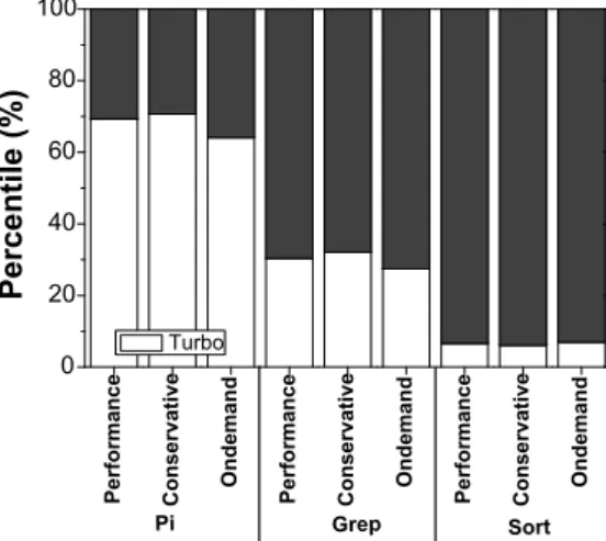
Interestingly, Figure 4(a) shows that the total energy consumption of the pi benchmark for the default frequency does not match the one corresponding to the performance-oriented governors, in spite of their similar execution times. The explanation lies in the processor ability to use the Turbo Boost capability when configured to employ an adaptive governor instead of a fixed frequency. The power consumption CDF for pi in Figure 6(a) shows the used power for the default CPU frequency is almost constant to 120 Watts for 80% of the job. As the CPU usage does not decrease during the execution of the pi application, this value represents the maximum power that the node can consume within a fixed frequency setting. However, the power consumption achieved by the two governors exceeds that of the default frequency, as emphasized by the pi CDF in Figure 6(a). This outcome is only possible if the governors take advantage of the CPU Turbo Boost capability, that is they employ a frequency higher than 2.53 GHz and in turn consume an increased amount of energy. Figure 9 provides an insight into the percentage of the job execution time spent by each governor with an enabled Turbo feature for each of the three applications. As previously anticipated, in the case of pi, the conservative governor invokes Turbo frequencies for 70% of the total time, while the ondemand governor requires
0 10 20 30 40 50 60 70 80 90 100 0 100 200 300 400 500 600 700 800 CPU Usage (%) Time (s) (a) Ondemand 0 10 20 30 40 50 60 70 80 90 100 0 100 200 300 400 500 600 700 800 CPU Usage (%) Time (s) (b) Conservative
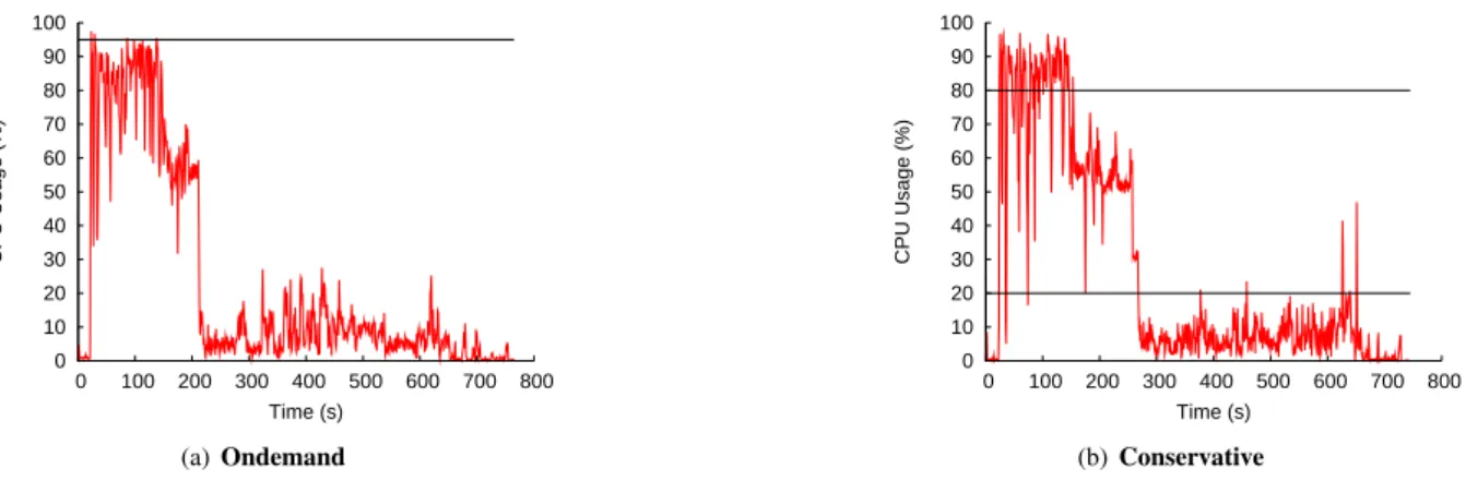
Figure 7. CPU usage on a Hadoop DataNode during the execution of the sort application under ondemand and conservative governors: The
ondemand governor is configured with the default up-threshold (i.e., 95%) while the conservative governor is configured with the default up and
down -threshold (i.e., 80% and 20%, respectively).
Turbo for 65% of the running time.
5.1.2. I/O-bound applications.
However, the conservative and ondemand governors behave differently for the sort application. As Figure 4 shows, when using the ondemand governor, Hadoop requires more time to sort the input data than when it is configured with the conservative governor. This longer running time also results in higher power consumption. To better understand how these two governors function, we analyze the CPU usage as a function of execution time on a single DataNode, during the sort benchmark (Figure 7). Both governors start the execution at the default frequency (2.53 GHz), but they adjust the CPU frequency according to the CPU usage and how it compares to predefined thresholds.
The ondemand governor uses as threshold a default value of 95%: when the CPU usage is greater than 95%, the CPU frequency is increased to the highest available frequency, i.e 2.53 GHz; if the CPU usage is less than this value, the governor gradually decreases the frequency to lower values. In the case of the sort benchmark, this policy allows Hadoop to run at the highest frequency in some points corresponding to the CPU usage peaks above the 95% threshold (Figure 7(a)). Nevertheless, the rest of the CPU-intensive phase of the sort application is executed at lower CPU frequencies, since the CPU usage during this phase is less than 95%. The conservative governor employs two thresholds for tuning the CPU frequency: an up-threshold set to 80% and a down-threshold of 20%. The frequency is progressively increased and decreased by comparing the system usage to the two thresholds: CPU usage peaks above the up-threshold result in upgrading the frequency to the next available value; when the usage goes below the down-threshold, the CPU switches to the next lower frequency. Figure 7(b) shows that the computational-intensive phase of the sort benchmark exhibits CPU usage peaks greater than 80%. This enables the conservative governor to keep the CPU at the highest frequency of 2.53 GHz during most of this phase. Also, the down-threshold allows the I/O-bound part of the application to be executed at low CPU frequencies.
The internal implementation of the two governors is also responsible for the overall variation in performance and consumed energy between the static 2.53 GHz setting and the dynamic governors detailed in Figure 4(c). Thus, in the case of sort, the conservative governor achieves a better runtime than ondemand, despite the fact that the latter governor should favour performance. While the improvement accounts for less than 5% of the execution time of the
ondemand governor, it can be explained by the fact that the conservative governor spends more time at the highest
frequency setting, speeding up the computational-intensive phases of sort. As most peaks in the CPU load do not reach the 95% threshold required by the ondemand governor, it cannot take advantage of the highest available frequency, leading to a worse application runtime. Energy-wise, this behaviour translates into a total energy gain when using the fixed 2.53 GHz frequency setting, on account on the longer execution time triggered by the ondemand governor. The
conservative governor is in this case the best choice for saving energy, as it enables the application to take advantage
of both high and low frequency settings, reducing the execution time of CPU-intensive phases and decreasing energy consumption during I/O-intensive ones.
ondemand conservative
Up-threshold 95% 80% Down-threshold - 20% Sampling window 0.01 Sec 0.08 Sec
Table 3. The configurable parameters in ondemand and conservative governors and their default values
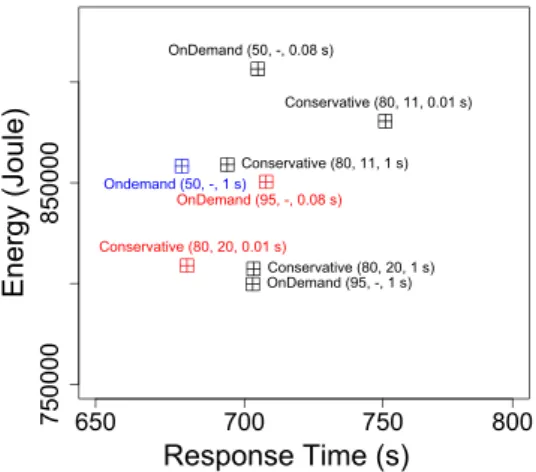
650 700 750 800 75000 0 8500 00 Response Time (s) Energy (Joule) Ondemand (50, -, 1 s) OnDemand (95, -, 0.08 s) OnDemand (95, -, 1 s) OnDemand (50, -, 0.08 s) Conservative (80, 20, 0.01 s) Conservative (80, 20, 1 s) Conservative (80, 11, 0.01 s) Conservative (80, 11, 1 s)
Figure 8. Effects of alternative configuration: Application runtime vs Energy consumption under ondemand and conservative governors. Each point represents the applications runtime and energy consumption under Governor(Up-threshold, Down-threshold, Sampling phase)
5.2. Impact of alternative governor configurations
The previous section suggests that the performance and energy behavior of Hadoop under the ondemand and
conservative are sensitive to the adjusted parameters. Therefore, to better understand the energy and performance
results the ondemand and conservative governors, we take a deeper look at the different parameters employed by both governors including up- and down-thresholds and sampling rate. Table 3 presents the different parameters and their default values employed in each governor.
We increase the sampling rate (i.e., the sampling rate determines how frequently the governor checks the current load and attempts to tune the CPU frequency) for both governors to 1 second and reduce the up-threshold parameter of the ondemand governor to 50%, to enforce using higher frequency and therefore achieve better performance. We also reduce the down-threshold of the conservative governor to 11%, to enforce using lower frequency and therefore achieve better energy efficiency. It is important to note that the choice of the 50% up-threshold for the ondemand governor is suggested by Figure 7, as the CPU usage is higher than 50% for almost 30% of the running time of the sort application. Similarly, the selection of the 11% down-threshold for the conservative governor is suggested as the CPU usage is less than 11% for almost 60% of the running time of the sort application, as shown in Figure 7.
When using the ondemand governor with the default up-threshold, Hadoop requires slightly less time to sort the input data when increasing the sampling rate from 0.01 Sec to 1 Sec. This effect, shown in Figure 8, can be explained by the reduced overhead of dynamically tuning the frequency as a result of a higher sampling rate. More importantly, when reducing the up-threshold to 50% while still using the default sampling rate, the performance slightly improves compared to the baseline (up-threshold 95%, sampling rate 0.01 Sec) but with slightly higher energy consumption. However, the performance of the sort application is significantly improved when the up-threshold is set to 50% and the sampling rate is set to 1 Sec. Even more, Hadoop requires slightly less time to sort the input data in these settings than when using the conservative governor with the default parameters.
On the other hand, when using the conservative governor with the default up- and down-thresholds and an in-creased sampling rate of 1 second, the performance of the sort application degrades, but with less energy consump-tion. Surprisingly, reducing the down-threshold to 11% does not bring any improvement for either the performance of the sort application or the energy consumption of the Hadoop cluster, regardless of the used sampling rate. The reason lies in the fact that a lower frequency is used for a longer time during the execution, thus increasing the application
P erf orm a nc e Co ns erva ti v e Onde m a nd P erf orm a nc e Co ns erva ti v e Onde m a nd P erf orm a nc e Co ns erva ti v e Onde m a nd 0 20 40 60 80 100 P erce nt il e ( %) Turbo Pi Grep Sort
Figure 9. Turbo Boost: The total usage of the Turbo feature for the duration of the application execution.
runtime and consequently the energy consumption.
5.3. Statically-configured frequencies
In this section we focus on the performance and powersave governors, which set the CPU to a fixed frequency, either the maximum available one, that is 2.53 GHz or the minimum 1.2 GHz, respectively. While they should exhibit similar behaviour with the fixed frequency, the performance governor features an interesting capability, that is to use Turbo Boost when executing heavy loads.
As far as the pi application is concerned, both performance and the fixed 2.53 GHz frequency setting deliver relatively similar running times. The Turbo feature allows the performance governor to go past the 2.53 GHz CPU frequency for 70% of the job execution time and thus consume more power, as confirmed by the CDF in Figure 6(a). A notable side effect is that the usage of the performance governor is less efficient from an energy standpoint (Fig-ure 4(a)). Fig(Fig-ure 6(b) shows a similar behaviour in the case of grep, as it exhibits a sufficiently similar workload. Consequently, for CPU-bound applications, performance-oriented governors provide a convenient alternative over a fixed frequency, when the user tends to favor performance. To achieve energy savings without significantly sacrificing execution time, the default kernel setting, the fixed maximum frequency still provides the best alternative. As for
sort, the generated CPU peaks account for a limited usage of the Turbo CPU feature, as detailed in Figure 9. As a
result, sort does not benefit from the performance governor in terms of energy, providing a better performance-energy tradeoff when using the 2.53 GHz setting or the conservative governor.
6. Fixed and configured policies vs coarse-grained tuning policies
Section 4 suggests that the performance and the total energy consumption of a Hadoop cluster under fixed CPU frequency strongly depends on the application’s CPU demands. CPU-intensive applications require higher CPU frequencies for better response time, but their usage does not necessarily result in a lower energy consumption. On the other hand, data-intensive applications require moderate CPU frequencies for better energy consumption, which do not necessarily imply better performance. Furthermore, as a MapReduce application comprises multiple subtasks, each of them requiring either computing power, disk I/O or bandwidth availability, there is a need for adaptive CPU frequency scaling policies that adjust the CPU frequency according to the CPU load. However, Section 5 suggests that Hadoop still behaves in an unpredictable manner, in terms of both performance and total energy consumption, under adaptive CPU frequencies (i.e., when applying the current state-of-the-art CPU governors) and even with different governor configurations.
In this section, we present a detailed comparative discussion on the performance and energy consumption in Hadoop with various DVFS policies: a coarse-grained governor tuning policy, a coarse-grained frequency tuning policy — when relying on static MapReduce phase detection, similar to [30][15] — and the various predefined CPU frequencies and governors.
sort pi wordcount k-means
number of samples/input data size ≃ 150GB 4,000 Million samples for each map ≃ 250GB ≃ 210GB number of map tasks 2475 maps 150 maps 3940 maps 3424 maps number of reduce tasks 78 reducers - 78 reducers 78 reducers
Table 4. Application configuration
6.1. Dynamic tuning policies
We study two coarse-grained frequency tuning policies:
• Dynamic CPU frequency. Similarly to the work in [15], we set the CPU frequency to the maximum one (i.e., 2.53GHz) during the map and reduce functions and to the minimum value otherwise (i.e., 1.2GHz).
• Dynamic governors tuning. We select the performance governor during the map and reduce functions and the
powersave governor otherwise. 6.2. Experimental setup
Large-scale testbed. On the testbed described in Section 3.1, we configured and deployed a Hadoop cluster using 40
nodes (1 master and 39 workers). The TaskTrackers were configured with 4 slots for running map tasks and 2 slots for executing reduce tasks.
Benchmarks. In addition to the sort and pi benchmarks, described in Section 3, we selected two more applications
from the PUMA benchmark [48]: wordcount and K-Means applications and configured the jobs as shown in Table 4.
K-means is a popular data mining algorithm that computes clusters of vectors based on the similarity between them;
the PUMA benchmark uses k-means to classify movies based on their ratings.
6.3. Results
Hereafter, we discuss the experimental results we obtained from running the four aforementioned benchmarks under 11 fixed CPU frequencies, 4 governors with their default parameters, 5 different configurations of the
onde-mand governor, 5 different configurations of the conservative governor, and the two dynamic policies introduced in
Section 6. We distinguish a total of 27 scenarios.
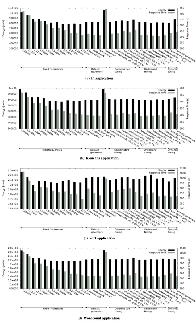
Figure 10(a) shows the results for the pi benchmark. We observe that when running the pi application under the performance-driven CPU frequencies or governors (i.e., 2.53 GHz, ondemand and performance), Hadoop requires relatively shorter time to complete the job with respect to other policies. The shortest application completion time is seen for ondemand(95, -, 0.4 Sec) — 211 seconds, ondemand (80, -, 3 Sec) — 213 seconds, and 2.53 Ghz — 216 seconds. Fixed CPU frequencies on the other hand still achieve the least energy consumption, as they allow Hadoop to complete the job with relatively short time and also without any extra usage of energy (e.g., no extra energy is used as the Turbo feature is disabled for fixed frequencies). We also observe that dynamic policies do not show good performance/energy improvement as the application runtime predominantly accounts for CPU usage.
Similarly, Hadoop requires shorter time to complete the k-means application under performance-driven CPU fre-quencies or governors (i.e., 2.53 GHz, ondemand and performance). The largest improvement in performance is 5%, achieved when using ondemand(80,-, 0.01 Sec) instead of the default CPU frequency 2.53GHz, but at a cost of energy reduction of 2%, as shown in Figure 10(b).
In general, for the sort application (see Figure 10(c)), the duration of the I/O phases is longer and the CPU load is lower than those in pi and k-means applications. For these reasons, the energy consumption under moderate CPU frequencies is reduced. Hence, adjusting the CPU frequency to 1.47 GHz and 2.00 GHZ saves smaller percentage of energy in contrast to 2.53 GHz. This, however, comes with a small degradation in the response time of 9.5%. Unfortunately, using alternative configurations and dynamic policies still result in no actual improvements of both energy and performance.
Since the wordcount application is a memory-intensive application and the main fraction of the running time is spent in the map phase, dynamic policies will not result in any actual performance and energy improvements. They may have the advantage of improving the performance, but this strongly depends on the performance of contributed
CPU frequencies and governors themselves. Moreover, the shortest job completion time is achieved using the
onde-mand governor (80, -, 0.01 Sec) — 537.5 seconds, and the lowest energy consumption is achieved when setting the
frequency to 2.13GHz (2, 159, 984 Joules), as shown in Figure 10(d).
6.3.1. Zoom on governor parameter sensitivity
We now focus exclusively on ondemand and conservative governors and study their sensitivity to different param-eters.
Impact of changing the sampling rate. Changing the sampling rate from 0.01 to 0.4 Sec1and 3 Sec, the aggressiveness
of CPU tuning is decreased for the ondemand governor. This results in a good performance improvement for CPU-dominant applications. On the contrary, changing the sampling rate from 0.08 to 0.4 Sec and 3 Sec, results in a worse performance for the conservative governor and energy consumption is increased further.
Impact of changing the up- and down-thresholds. When the up-threshold is modified from 95% to 80% for the ondemand governor, the application takes advantage of higher frequencies for a longer fraction of time and thus, the
performance is improved and energy consumption is decreased. Similarly to the ondemand governor, changing the up-threshold from 80% to 60% and the down-threshold from 20% to 40% for the conservative governor results in practical performance and energy improvements.
6.3.2. Zoom on dynamic policies results
We now study the implications of the two dynamic policies on the energy and performance in Hadoop. For all applications, dynamic frequencies policy not only outperforms dynamic governors policy but also reduces the energy consumption of Hadoop cluster. It was expected that the energy consumption when using 2.53 GHz is better than when using the performance governor, as explained in Section 4.
6.3.3. Summary
The results shown in this section confirm that static phases based solutions are ineffective at saving energy in Hadoop clusters and also at improving performance. Also, by adjusting the up and down -threshold and the sampling rate, Hadoop still behaves unpredictably in terms of performance and energy consumption. Therefore, a new adaptive approach, much beyond the current state of governors and phase-based solutions, is needed. Such approach should be specifically tailored to match MapReduce application types and execution stages.
7. Conclusion and Future Work
Energy efficiency has started to severely constrain the design and the way data-centers are operated, becoming a key research direction in the development of cloud infrastructures. As processing huge amounts of data is a typical task assigned to large-scale cloud platforms, several studies have been dedicated to improving power consumption for data-intensive cloud applications. In this study, we focus on MapReduce and we investigate the impact of dynamically scaling the frequency of compute nodes on the performance and energy consumption of a Hadoop cluster. We provide a detailed evaluation of a set of representative MapReduce workloads, highlighting a significant variation in both the performance and power consumption of the applications with different governors.
Furthermore, our results reveal that the current CPU governors do not exactly reflect their design goal and may even become ineffective at improving power consumption for Hadoop clusters. In addition, we unveil the correlations between the power efficiency of a Hadoop deployment, application performance and power-management mechanisms,
1We chose the value of 0.4 as an alternative sampling rate to have similar value to the heartbeat interval. Hadoop adjusts the heartbeat interval
according to the cluster size. The heartbeat interval is calculated so that the JobTracker receives a min heartbeat interval of 100 heartbeat messages every second (by default). Moreover, the min heartbeat interval limits the heartbeat interval to not be smaller than 300 milliseconds, corresponding to the cluster size of 30 nodes. The heart beat interval in Hadoop is computed as:
heartbeat interval= max((1000 × cluster size ÷ number heartbeat per second), min heartbeat interval) 16
(a) Pi application
(b) K-means application
(c) Sort application
(d) Wordcount application
Figure 10. Application runtime vs Energy consumption under various policies.
such as DVFS or Turbo capabilities. We believe the insights drawn from this paper can serve as guidelines for efficiently deploying and executing data-intensive applications in large-scale data-centers.
As future work, we intend to explore different techniques and approaches to optimize power management in Hadoop clusters. As a first step, we are currently investigating the possibility of building dynamic frequency tuning tools specifically tailored to match MapReduce application types and execution stages.
8. Acknowledgments
This work is supported by the ANR MapReduce grant (ANR-10-SEGI-001) and the H´em´era INRIA Large Wingspan-Project (see http://www.grid5000.fr/mediawiki/index.php/Hemera).
Experiments presented in this paper were carried out using the Grid’5000 testbed, supported by a scientific interest group hosted by Inria and including CNRS, RENATER and several Universities as well as other organizations (see http://www.grid5000.fr/).
References
[1] J. Hamilton, Cost of Power in Large-Scale Data Centers, http://perspectives.mvdirona.com/2008/11/28/ CostOfPowerInLargeScaleDataCenters.aspx (2008).
[2] A. M. Sampaio, J. G. Barbosa, Towards high-available and energy-efficient virtual computing environments in the cloud, Future Generation Comp. Syst. 40 (2014) 30–43. doi:10.1016/j.future.2014.06.008.
URL http://dx.doi.org/10.1016/j.future.2014.06.008
[3] J. Xu, J. Fortes, Multi-objective virtual machine placement in virtualized data center environments, in: Green Computing and Communica-tions (GreenCom), 2010 IEEE/ACM Int’l Conference on Int’l Conference on Cyber, Physical and Social Computing (CPSCom), 2010, pp. 179–188.
[4] J. Xu, J. Fortes, A multi-objective approach to virtual machine management in datacenters, in: Proceedings of the 8th ACM International Conference on Autonomic Computing, ICAC ’11, 2011.
[5] Y. Lee, A. Zomaya, Energy efficient utilization of resources in cloud computing systems, The Journal of Supercomputing 60 (2). doi:10.1007/s11227-010-0421-3.
[6] N. Maheshwari, R. Nanduri, V. Varma, Dynamic energy efficient data placement and cluster reconfiguration algorithm for mapreduce frame-work, Future Generation Comp. Syst. 28 (1) (2012) 119–127. doi:10.1016/j.future.2011.07.001.
URL http://dx.doi.org/10.1016/j.future.2011.07.001
[7] I. Goiri, K. Le, T. D. Nguyen, J. Guitart, J. Torres, R. Bianchini, Greenhadoop: Leveraging green energy in data-processing frame-works, in: Proceedings of the 7th ACM European Conference on Computer Systems (EuroSys ’12), Bern, Switzerland, 2012. doi:http://doi.acm.org/10.1145/1272996.1273005.
[8] I. n. Goiri, K. Le, M. E. Haque, R. Beauchea, T. D. Nguyen, J. Guitart, J. Torres, R. Bianchini, Greenslot: Scheduling energy consumption in green datacenters, in: Proceedings of 2011 International Conference for High Performance Computing, Networking, Storage and Analysis, SC ’11, 2011, pp. 20:1–20:11.
[9] G. von Laszewski, L. Wang, A. Younge, X. He, Power-aware scheduling of virtual machines in dvfs-enabled clusters, in: Cluster Computing and Workshops, 2009. CLUSTER ’09. IEEE International Conference on, 2009, pp. 1–10.
[10] S. Khan, I. Ahmad, A cooperative game theoretical technique for joint optimization of energy consumption and response time in computa-tional grids, Parallel and Distributed Systems, IEEE Transactions on 20 (3) (2009) 346–360.
[11] J. Dean, S. Ghemawat, MapReduce: simplified data processing on large clusters, Communications of the ACM 51 (1) (2008) 107–113. [12] The Apache Hadoop Project, http://www.hadoop.org (2014).
[13] M. Cardosa, A. Singh, H. Pucha, A. Chandra, Exploiting spatio-temporal tradeoffs for energy-aware mapreduce in the cloud, in: Proceedings of the 2011 IEEE 4th International Conference on Cloud Computing, CLOUD ’11, Washington, DC, USA, 2011, pp. 251–258.
[14] Y. Chen, A. Ganapathi, R. H. Katz, To compress or not to compress - compute vs. io tradeoffs for mapreduce energy efficiency, in: Proceed-ings of the first ACM SIGCOMM workshop on Green networking, Green Networking ’10, ACM, New York, NY, USA, 2010, pp. 23–28. doi:10.1145/1851290.1851296.
URL http://doi.acm.org/10.1145/1851290.1851296
[15] T. Wirtz, R. Ge, Improving mapreduce energy efficiency for computation intensive workloads, in: Proceedings of 2011 Interna-tional Green Computing Conference and Workshops (IGCC’11), Green Networking ’10, IEEE, New York, NY, USA, 2011, pp. 1–8. doi:10.1145/1851290.1851296.
URL http://doi.acm.org/10.1145/1851290.1851296
[16] L. Shen, T. Abdelzaher, M. Yuan, Tapa: Temperature aware power allocation in data center with map-reduce, in: Proceedings of 2011 International Green Computing Conference and Workshops (IGCC’11), Green Networking ’10, IEEE, New York, NY, USA, 2011, pp. 1–8. doi:10.1145/1851290.1851296.
URL http://doi.acm.org/10.1145/1851290.1851296
[17] S. Ibrahim, D. Moise, H.-E. Chihoub, A. Carpen-Amarie, L. Boug, G. Antoniu, Towards efficient power management in mapreduce: Investi-gation of cpu-frequencies scaling on power efficiency in hadoop, in: F. Pop, M. Potop-Butucaru (Eds.), Adaptive Resource Management and Scheduling for Cloud Computing, Lecture Notes in Computer Science, Springer International Publishing, 2014, pp. 147–164.
URL http://dx.doi.org/10.1007/978-3-319-13464-2_11
[18] F. Pop, M. Potop-Butucaru (Eds.), Adaptive Resource Management and Scheduling for Cloud Computing, Vol. 8907 of Lecture Notes in Computer Science (LNCS)/ Theoretical Computer Science and General Issues, Springer, 2015.
[19] Redhat: Using CPUfreq Governors, https://access.redhat.com/site/documentation/en-US/Red\_Hat\_Enterprise\ _Linux/6/html/Power\_Management\_Guide/cpufreq\_governors.html (2014).
[20] Y. J´egou, S. Lant´eri, J. Leduc, N. Melab, G. Mornet, R. Namyst, P. Primet, B. Quetier, O. Richard, E.-G. Talbi, T. Ir´ea, Grid’5000: a large scale and highly reconfigurable experimental Grid testbed., International Journal of High Performance Computing Applications 20 (4) (2006) 481–494.
[21] H. Jin, S. Ibrahim, L. Qi, H. Cao, S. Wu, X. Shi, The mapreduce programming model and implementations, Cloud computing: Principles and Paradigms (2011) 373–390.
[22] C. Ranger, R. Raghuraman, A. Penmetsa, G. Bradski, C. Kozyrakis, Evaluating mapreduce for multi-core and multiprocessor systems, in: Proceedings of the 2007 IEEE 13th International Symposium on High Performance Computer Architecture (HPCA-13), Phoenix, Arizona, USA, 2007, pp. 13–24. doi:10.1109/HPCA.2007.346181.
[23] B. He, W. Fang, Q. Luo, N. K. Govindaraju, T. Wang, Mars: a mapreduce framework on graphics processors, in: Proceedings of the 17th international conference on Parallel architectures and compilation techniques, Toronto, Ontario, Canada, 2008, pp. 260–269. doi:http://doi.acm.org/10.1145/1454115.1454152.
[24] S. Ibrahim, H. Jin, L. Lu, L. Qi, S. Wu, X. Shi, Evaluating mapreduce on virtual machines: The hadoop case, in: Proceedings of the 1st International Conference on Cloud Computing (CLOUDCOM’09), Beijing, China, 2009, pp. 519–528.
[25] L. Wang, J. Tao, R. Ranjan, H. Marten, A. Streit, J. Chen, D. Chen, G-hadoop: Mapreduce across distributed data centers for data-intensive computing, Future Gener. Comput. Syst. 29 (3) (2013) 739–750. doi:10.1016/j.future.2012.09.001.
URL http://dx.doi.org/10.1016/j.future.2012.09.001
[26] S. Ibrahim, H. Jin, L. Lu, S. Wu, B. He, L. Qi, Leen: Locality/fairness-aware key partitioning for mapreduce in the cloud, in: Proceedings of the 2010 IEEE Second International Conference on Cloud Computing Technology and Science (CLOUDCOM’10), Indianapolis, USA, 2010, pp. 17–24. doi:http://dx.doi.org/10.1109/CloudCom.2010.25.
[27] Y. Kwon, M. Balazinska, B. Howe, J. Rolia, Skew-resistant parallel processing of feature-extracting scientific user-defined func-tions, in: Proceedings of the 1st ACM symposium on Cloud computing, Indianapolis, Indiana, USA, 2010, pp. 75–86. doi:http://doi.acm.org/10.1145/1807128.1807140.
[28] S. Ibrahim, H. Jin, L. Lu, B. He, G. Antoniu, S. Wu, Maestro: Replica-aware map scheduling for mapreduce, in: Proceedings of the 12th IEEE/ACM International Symposium on Cluster, Cloud and Grid Computing (CCGrid 2012), Ottawa, Canada, 2012, pp. 59–72. doi:http://doi.acm.org/10.1145/1272996.1273005.
[29] M. Zaharia, D. Borthakur, J. Sen Sarma, K. Elmeleegy, S. Shenker, I. Stoica, Delay scheduling: a simple technique for achieving locality and fairness in cluster scheduling, in: Proceedings of the 5th ACM European Conference on Computer Systems (EuroSys’10), Paris, France, 2010, pp. 265–278. doi:http://doi.acm.org/10.1145/1755913.1755940.
[30] S. Ibrahim, H. Jin, L. Lu, B. He, S. Wu, Adaptive disk i/o scheduling for mapreduce in virtualized environment, in: Proceedings of the 2011 International Conference on Parallel Processing (ICPP’11), Taipei, Taiwan, 2011, pp. 335–344. doi:http://dx.doi.org/10.1109/ICPP.2011.86. [31] H. Jin, X. Ling, S. Ibrahim, W. Cao, S. Wu, G. Antoniu, Flubber: Two-level disk scheduling in virtualized environment, Future Generation
Comp. Syst. 29 (8) (2013) 2222–2238. doi:10.1016/j.future.2013.06.010. URL http://dx.doi.org/10.1016/j.future.2013.06.010
[32] H. Amur, J. Cipar, V. Gupta, G. R. Ganger, M. A. Kozuch, K. Schwan, Robust and flexible power-proportional storage, in: Proceedings of the 1st ACM symposium on Cloud computing, SoCC ’10, ACM, New York, NY, USA, 2010, pp. 217–228. doi:10.1145/1807128.1807164. URL http://doi.acm.org/10.1145/1807128.1807164
[33] R. T. Kaushik, M. Bhandarkar, Greenhdfs: towards an energy-conserving, storage-efficient, hybrid hadoop compute cluster, in: Proceedings of the 2010 international conference on Power aware computing and systems, HotPower’10, USENIX Association, Berkeley, CA, USA, 2010, pp. 1–9.
URL http://dl.acm.org/citation.cfm?id=1924920.1924927
[34] J. Kim, J. Chou, D. Rotem, Energy proportionality and performance in data parallel computing clusters, in: Proceedings of the 23rd interna-tional conference on Scientific and statistical database management, SSDBM’11, Springer-Verlag, Berlin, Heidelberg, 2011, pp. 414–431. URL http://dl.acm.org/citation.cfm?id=2032397.2032431
[35] J. Leverich, C. Kozyrakis, On the energy (in)efficiency of hadoop clusters, SIGOPS Oper. Syst. Rev. 44 (1) (2010) 61–65.
[36] E. Thereska, A. Donnelly, D. Narayanan, Sierra: practical power-proportionality for data center storage, in: Proceedings of the sixth confer-ence on Computer systems, EuroSys ’11, ACM, New York, NY, USA, 2011, pp. 169–182. doi:10.1145/1966445.1966461.
URL http://doi.acm.org/10.1145/1966445.1966461
[37] N. Vasi´c, M. Barisits, V. Salzgeber, D. Kostic, Making cluster applications energy-aware, in: Proceedings of the 1st workshop on Automated control for datacenters and clouds, ACDC ’09, ACM, New York, NY, USA, 2009, pp. 37–42. doi:10.1145/1555271.1555281.
URL http://doi.acm.org/10.1145/1555271.1555281
[38] W. Lang, J. M. Patel, Energy management for mapreduce clusters, Proc. VLDB Endow. 3 (1-2) (2010) 129–139. URL http://dl.acm.org/citation.cfm?id=1920841.1920862
[39] N. Zhu, L. Rao, X. Liu, J. Liu, H. Guan, Taming power peaks in mapreduce clusters, in: Proceedings of the ACM SIGCOMM 2011 conference, SIGCOMM ’11, ACM, New York, NY, USA, 2011, pp. 416–417.
[40] Y. Chen, L. Keys, R. H. Katz, Towards energy efficient mapreduce, Tech. Rep. UCB/EECS-2009-109, EECS Department, University of California, Berkeley (Aug 2009).
URL http://www.eecs.berkeley.edu/Pubs/TechRpts/2009/EECS-2009-109.html
[41] Y. Chen, S. Alspaugh, D. Borthakur, R. Katz, Energy efficiency for large-scale mapreduce workloads with significant interactive analysis, in: Proceedings of the 7th ACM European Conference on Computer Systems (EuroSys ’12), Bern, Switzerland, 2012. doi:http://doi.acm.org/10.1145/1272996.1273005.
[42] L. Mashayekhy, M. M. Nejad, D. Grosu, D. Lu, W. Shi, Energy-aware scheduling of mapreduce jobs, in: Big Data (BigData Congress), 2014