HAL Id: hal-01609082
https://hal.archives-ouvertes.fr/hal-01609082
Submitted on 3 Oct 2017
HAL is a multi-disciplinary open access archive for the deposit and dissemination of sci-entific research documents, whether they are pub-lished or not. The documents may come from teaching and research institutions in France or
L’archive ouverte pluridisciplinaire HAL, est destinée au dépôt et à la diffusion de documents scientifiques de niveau recherche, publiés ou non, émanant des établissements d’enseignement et de recherche français ou étrangers, des laboratoires
Thorough IoT testbed Characterization: from
Proof-of-concept to Repeatable Experimentations
Georgios Papadopoulos, Antoine Gallais, Guillaume Schreiner, Emery Jou,
Thomas Noel
To cite this version:
Georgios Papadopoulos, Antoine Gallais, Guillaume Schreiner, Emery Jou, Thomas Noel. Thorough IoT testbed Characterization: from Proof-of-concept to Repeatable Experimentations. Computer Networks, Elsevier, 2017, 119, pp.86 - 101. �10.1016/j.comnet.2017.03.012�. �hal-01609082�
Thorough IoT testbed Characterization:
from Proof-of-concept to Repeatable Experimentations
Georgios Z. Papadopoulosa,b, Antoine Gallaisa,
Guillaume Schreinera, Emery Jouc, Thomas Noela
aICube Laboratory, University of Strasbourg, France bIRISA, T´el´ecom Bretagne, Institut Mines-T´el´ecom, France
cInstitute for Information Industry, Taipei, Taiwan
Abstract
In this paper, we explore the role of simulators and testbeds in the devel-opment procedure of protocols or applications for Wireless Sensor Networks (WSNs) and Internet of Things (IoT). We investigate the complementarity between simulation and experimentation studies by evaluating latest features available among open testbeds (e.g., energy monitoring, mobility). We show that monitoring tools and control channels of testbeds allow for identifica-tion of crucial issues (e.g., energy consumpidentifica-tion, link quality) and we identify some opportunities to leverage those real-life obstacles. In this context, we insist on how simulations and experimentations can be efficiently and suc-cessfully coupled with each other in order to obtain reproducible scientific results, rather than sole proofs-of-concept. Indeed, we especially highlight the main characteristics of such evaluation tools that allow to run multi-ple instances of a same experimental setup over stable and finely controlled components of hardware and real-world environment. For our experiments, we used and evaluated the FIT IoT-LAB facility. Our results show that such open platforms, can guarantee a certain stability of hardware and en-vironment components over time, thus, turning the unexpected failures and changing parameters into core experimental parameters and valuable inputs for enhanced performance evaluation.
Keywords: IoT, WSNs, performance evaluation, reproducibility,
repeatability, network simulators, experimentation testbeds.
1. Introduction
Wireless Sensor Networks (WSNs) and Internet of Things (IoT) are ab-sorbing more and more attention from the research community due to their wide range of applications (e.g., wildlife monitoring [1], environment mon-itoring in coal mines [2], telemedicine [3]). Experiences through the past real-world deployments [4], [5], [6], [7] have shown that continuing directly with deployments can lead to various unexpected issues such as node failure or network disconnection. Moreover, a majority of Ad Hoc, WSN and IoT networks pose significant challenges due to the hardware limitations of sen-sor nodes (e.g., processen-sor, memory or battery) or constrained environment in which the nodes are deployed (e.g., ocean, mountains). It is therefore crucial to verify the protocols at each stage of design, development and implemen-tation, either by utilizing simulators or by employing testbeds, before having them deployed in real-world environments.
However, environments that are targeted by wireless sensor networks are often application-specific and too complex to be reproduced precisely. With replications, independent researchers may address a scientific hypothesis and construct evidence for or against it.
Simulators allow researchers to provide a proof-of-concept for new solu-tions in a virtual environment by avoiding time-consuming, heavyweight or expensive real-world experimentation. Furthermore, the majority of the sim-ulation models can not capture precisely the real-world complexity [8], [7]. Our purpose is to show that this step is not sufficient to assess the consistency of a solution all the more so as low cost devices have steered researchers to enrich performance evaluation with testbeds.
On the other hand, experimental evaluation (over custom or open testbeds) exhibits potential unexpected problems (e.g., node failures, network discon-nections). In addition to performing well over a given testbed, a sound in vitro deployment should however allow for reproducibility of the results. Else, such evaluations would simply lead to proofs-of-concept whose translation to real-world scenarios would not be guaranteed.
Designing and setting up a complete Ad Hoc or WSN system under realis-tic conditions that can support robust applications is a very complex task [9]. First, an appropriate plan of deployment is required from researchers and production system architects. Then, in order to initially confirm their con-cept or model, number of tools are required for validation and real-world experiments.
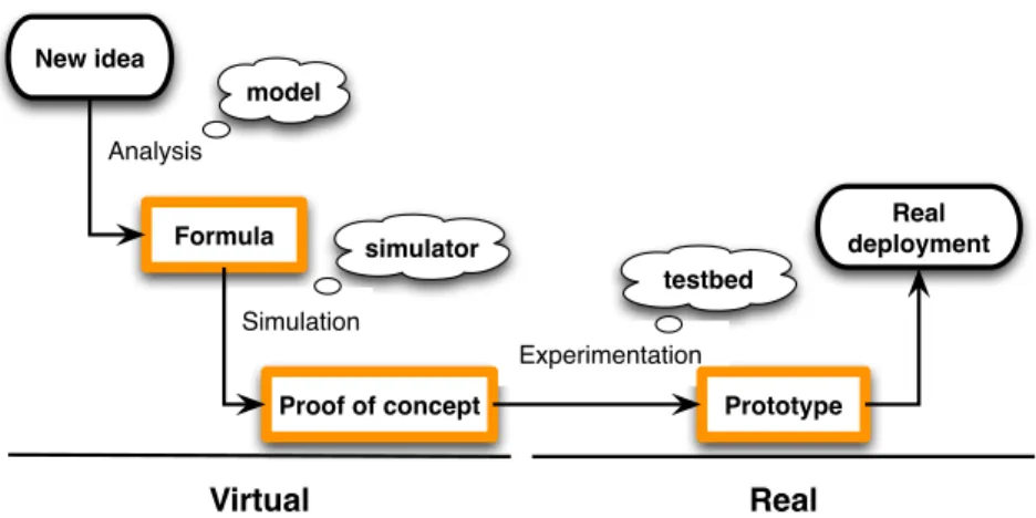
Experimentation Simulation Virtual Real New idea Real deployment Formula Analysis
Proof of concept Prototype
model
simulator
testbed
Figure 1: A typical research process cycle.
In wireless networks, verification of theoretical analysis is a vital step during the protocol development. Simulators and testbeds are two important and complementary design and validation tools; an ideal development process should start from the theoretical analysis of the protocol providing bounds and indication of its performance, verified and refined by simulators and finally confirmed in a testbed (see Figure 1) [10]. In the community, there are number of simulators [11] and open testbeds [12] available for researchers to perform simulation or experimental evaluation of their solutions. However, there is always a concern about the retrieved results from such tools that they may not reflect the mathematical derivations or accurate behavior.
Our investigation is based on a previous article [13], in which we stud-ied the role of simulators and testbeds in the research process cycle, and we identified the means to strengthen their complementarity. Moreover, we exposed to what extent experimental campaigns can be efficiently conducted and provide essential values to theoretical estimations and to simulation per-formance. We thus explored the adding value of testbeds in the design and development of protocols for IoT networks. We here concentrate on facili-ties that allow to evaluate communication protocols and services along with associated methodology.
In this article, we first focus on the evaluation methodologies provided by the research community. To this aim, we analyze a large set of statis-tics on articles published in Ad Hoc and WSNs related top representative conferences. Since experiments on testbeds seem to have become a must
for verification of new models and protocols, we debate the meaning of a proof-of-concept, and the selection of the appropriate validation tool.
For this campaign, we focused on the FIT IoT-LAB1, a very large-scale
and open experimental testbed. Thus, to bootstrap our investigation, we first perform an exhaustive radio link characterization as well as an evaluation of the connectivity under real-world conditions. More specifically, we employed various hardware (e.g., WSN430, M3) and topologies. Moreover, we evalu-ated the performance of the IEEE 802.15.4-2015 standard [14] in these real-world environments. We aimed at demonstrating to what extent some of the simulation setup and conditions from reality could be emulated. We describe how successful testbed experimentations could be translated into real-world deployments (e.g., exposing a precise calculation of energy consumption) as we investigate link quality and stability, density of the wireless network and usage of mobile robots. Finally, we discuss and highlight the key features of simulators and experimentation platforms.
The contributions presented in this paper are as follows:
• A thorough radio link characterization (e.g., neighborhood density, con-nectivity, and link quality), in order to allow researchers and engineers to identify high-quality bidirectional links and thus determine appro-priate network density,
• Identification of stable links over time for providing repeatable setups, thus obtaining reproducible results,
• Introduction of mobility in IoT testbeds, ranging from the basic opera-tions (e.g., automatic recharging, trajectory planning) to the advanced usage of such devices (e.g., handling drifts over predefined trajectories). The remainder of this paper is organized as follows. In Section 2, we motivate our investigation by discussing the actual combined use of simula-tors and testbeds. Section 3 provides the detailed description with all the necessary features of the FIT IoT-LAB testbed. Section 4, presents a set of meaningful experimental campaigns that have been conducted over ICube testbed. In Section 5, we discuss and highlight the key features of simula-tors and experimentation. Finally, in Section 6 we provide the concluding remarks of our work and certain suggestions for future work.
2. Motivation
In [15], we compiled a large set of statistics on literature review of 674 articles, out of which 596 are indeed related to with Ad Hoc, WSN and IoT (see Figure 2a), published in top representative conferences that are strongly related with Ad Hoc, WSN and IoT research areas over the 2008-2013 pe-riod. More specifically, we went through all articles that have been published at the ACM/IEEE International Conference on Information Processing in Sensor Networks (IPSN), ACM Annual International Conference on Mobile Computing and Networking (MobiCom), ACM International Symposium on Mobile Ad Hoc Networking and Computing (MobiHoc) and ACM Confer-ence on Embedded Networked Sensor Systems (SenSys) conferConfer-ences in order to determine the performance evaluation methodologies that researchers fol-low. In particular, we examine the proportion of simulation, experimental and mathematical (i.e., modeling or analysis) evaluated works.
2.1. More and more experimentations over testbeds
Our investigation demonstrates that there is a tendency for more and more researchers to rely on custom or open testbeds in order to evaluate the performance of their proposals. The percentage of simulation versus experiment-based studies (with respect to 596 studied articles) is illustrated in Figure 2b. As can be observed, while simulations and experiments used to be equally deployed until 2009, the usage of simulations is decreasing every year (except in 2011) while experimentations still remain present at a relatively stable rate. Moreover, our investigation shows that the majority (i.e., 561) of the articles include theoretical study in their solutions and only one out of five (i.e., 20.3%) articles examines all three phases of the research process cycle (i.e., analysis, simulation and experimentation), as shown on Figure 2c [15] (with respect to 596 studied papers). Finally, while half of the papers provide simulation evaluation (284), two third of them (392) verify their proposals by employing experimental evaluation.
The main reason to explain this phenomenon could be the quite low costs now induced by a testbed setup. However, running real experiments still re-mains time consuming (i.e., to flash, reboot and (re)load the firmware, debug and eventually to retrieve the measurements) and requires dedicated skills and knowledge. On the other hand, most of simulators provide abstraction interfaces (e.g., less low-level functions and electronic references) to hide the
2008 2009 2010 2011 2012 2013 0 20 40 60 80 100 120 140 Nu mb er of art icl es Total
Ad-Hoc & WSN related
(a) Number of articles per year (all conferences are considered).
2008 2009 2010 2011 2012 2013 Conference proceedings 0 20 40 60 80 100 Pro po rti on (% ) Simulation Experiment
(b) Total simulation versus experimentation evaluated articles.
S, 3 S & E, 10 E, 22 M, 51 M & S & E, 121 M & S, 150 M & E, 239 (c) Use of Mathematics (M), Simulations (S), Experiments (E)
in validation procedures.
Figure 2: Published articles in ACM/IEEE IPSN, ACM MobiCom, ACM MobiHoc and ACM SenSys from 2008 to 2013 [15].
complexity of embedded systems programming while testbeds do not. Simu-lation also allows scientists to isolate different factors by tuning configurable parameters independently while experimentations lead researchers to real en-vironments and materials with constraints that are hard to model in existing simulators. Moreover, simulation tools facilitate the obtention of all the re-quired results and ensure efficient retrieval of exploitable information (e.g., logging operations such as printing of data and calculations) without any impact on the node functioning (e.g., energy consumption, processing time). Furthermore, each information can be associated with a precise timestamp (all nodes sharing the same clock). These features enable very detailed and accurate evaluation of any metric (e.g., one-hop delay), and allow for corre-lation of the data.
However, in order to enable such features, simulations have to hide the limitations and constraints imposed by actual components. For instance, most simulators provide unlimited memory and computation resources and do not take into account the probability of node failure. In this context it is often tricky for users to evaluate the realism and complexity of their contri-butions. Many researchers develop extensively complex and, thus, unrealistic mechanisms that might display very promising simulation results.
2.2. Bridging the gap between simulations and experimentations
Emulators such as TOSSIM [16] or COOJA [17] were designed to bridge the gap between simulation and experimentation, by remaining as close as possible to programming conditions of real embedded systems. To do so, they rely on the same code for both simulation and experimental campaigns, and thus allow users to apprehend the specificities of this field as early as at the simulation setup. However, many parameters relative to the radio environ-ment (e.g., link properties and evolution over time, interferences) and node behavior (e.g., failure) can not be modeled accurately. Thus, even though the code complexity remains identical, the deployment conditions and ensuing effects can only be apprehended and experienced through experimentation.
However, when proceeding through testbed steps, researchers should not expect the same guarantees and validations as the ones provided by the sim-ulators. Many parameters of any experiment remain out of control. The en-vironmental radio activity varies due to the interpolation of external features (e.g., mobile phones, wireless devices and access points). Energy consump-tion depends on hardware or even weather condiconsump-tions.
Moreover, setting up such facilities can be considered as difficult and time-consuming, mobilizing human resources other than researchers. Nowadays, these obstacles can be mitigated by using open testbeds that allow to gain access to real hardware and already deployed experimentation networks [12]. Furthermore, we may advocate that the most important difference be-tween open and custom testbeds lies in the guarantees that each of them can provide. While custom experimentation platforms produce proof-of-concepts and early prototypes, open testbeds are expected to allow multiple instances of a same experimental setup, potentially by researchers other than those having deployed the testbed. Indeed, regarding simulations, any researcher can use a given simulator to test a proposed solution with a given simulation setup. If similar results can be obtained by anyone having access to the same
simulator, with the same proposed solution and the same complete simula-tion setup, then the obtained results are considered as scientific results by the community. This should also apply for open testbeds.
2.3. Towards more trusted testbeds
Reproducibility is the ultimate standard by which scientific claims are evaluated and criticized. In order to increase the confidence, certain stabil-ity must be preserved throughout the development procedure (i.e., analysis, simulation and experimentation) of an application or protocol (see Figure 1). Stability is a relevant concept among these steps and we aim at investigating to what extent it can be ensured in open testbeds. Experiments should also be stable over time as well as in terms of topology changes and operation of communication links. For instance, if one experiment running on Friday were to lead to different observations from another run on Monday, then the different conditions that issued this situation should be characterized. Else, obtained results can not be considered as scientific since the manda-tory conditions for their reproducibility can not be provided. In case there are variations in testbed experiments, they should be due to the used hardware only, in order to reflect the complexity and heterogeneity of target objects. Hence, researchers should continue with real deployments once they reach stability of their testbed solution.
2.3.1. Stability of topology: the example of link quality
In [18], authors report results of measurements on FIT IoT-LAB where both Received Signal Strength Indication (RSSI) and Link Quality Indicator (LQI) were analyzed to find the best way to discriminate good links from weak ones. Authors aim at efficiently estimating Packet Reception Ratio (PRR) according on the observed RSSI and LQI values. Even though RSSI can indicate some possible anomalous behaviour of sensor nodes, their ex-periments confirm that RSSI fails to discriminate link categories. Therefore, the proposed solution allows to find PRR for a given level of LQI.
2.3.2. Stability of topology: the example of mobility
Applications such as e-health with wearable sensors (i.e., eldercare and well-being) [19], cargos containers [20], automotive industry or even airport logistics all share similar requirements, including mobile devices. Thus, the upcoming standards should consider the additional constraints due to the nodes movement within the operation of the network. For instance, number
of disconnections from the infrastructure may cause certain disruptions to the functionality of the network, and consequently would degrade the net-work performance and reliability. As a result, simulation and experimental performance evaluation of the envisioned mobility-aware use cases prior to the real deployments would be required.
The majority of existing and used simulators allow to use and create mobility models. However, testing and executing such scenarios during an experimentation procedure requires to involve and combine advanced and intelligent technologies such as robots. Consequently, very few of the widely popular open platforms do support mobility [21] Actually, numerous chal-lenges need to be addressed when having mobile robots in a testbed, namely, charging, remote administration and maintenance of the robots. Indeed, robots must be able to reach their docking stations automatically. Con-versely, remote users must be able to interact with robots over reliable links (e.g., WiFi). Even though these challenges can be addressed, testbed admin-istrators then face the issue of localizing mobile devices in order to allow for repeatable trajectories. Indoor deployments can not rely on GPS solutions and thus impose distance approximations to be computed based on other available inputs (e.g., received signal strength intensity) or on costly tech-nologies (e.g., 3D camera with range detector sensors for the mapping of the environment).
However, even with perfect localization of all robots, trajectories would be very difficult to replay, especially due to the odometry drift. Some 3D cameras using range detector sensor aim at handling this drift. Still they lack to compute the path where not enough landmarks exist in open-space and large-scale environments.
3. FIT IoT-LAB Facilities
In this section, we introduce FIT IoT-LAB, a large scale and an open access multi-user testbed. FIT IoT-LAB is the evolution and extension of the SensLAB [22] testbed (2010-2013). It offers facilities suitable for testing small wireless sensor devices and heterogeneous communicating objects. FIT IoT-LAB provides full control of network nodes and direct access to the gateways to which nodes are connected, allowing researchers to precisely monitor nodes energy consumption and network-related metrics. Furthermore, FIT IoT-LAB platform comes with all the necessary tools (e.g., RSSI mapping, link stability and quality analyzer) to ensure that the environmental conditions of
Node Grenoble Lille Rocquencourt Strasbourg Rennes Paris Total WSN430 (800MhZ) 256 - - 256 - - 512 WSN430 (2.4GhZ) - 256 120 - 256 - 632 Cortex M3 384 320 24 120 - 90 938 Cortex A8 256 - 200 24 - 70 550 Open Host 32 64 - - - - 96 Total 928 640 344 400 256 160 2728
Table 1: Testbeds distribution of nodes
the facilities are fulfilled before launching experiments. It therefore provides quick experiments deployment, along with easy results collection, evaluation and consequently analysis. The testbed is composed of 2728 wireless sensor nodes distributed over six different sites in France, Inria Grenoble (928), Inria Lille (640), ICube Strasbourg (400), Inria Rocquencourt (344), Inria Rennes (256) and Mines-Telecom Paris (160). The wireless devices are allocated within different topologies and environments (e.g., isolated or real-world) throughout all sites. Finally, some of the platforms offer mobile robots to evaluate mobility-based solutions.
3.1. An IoT-LAB hardware
A global IPv4/IPv6 networking backbone provides full control of nodes and direct access to the gateways to which FIT IoT-LAB nodes are con-nected, allowing researchers to monitor nodes energy consumption and an-alyze network-related metrics (e.g., end-to-end delay, reliability). Further-more, IoT-LAB infrastructure comprises a set of IoT-LAB nodes, where each node consists of three main components, the open wireless sensor node, gate-way and control node respectively.
In order to meet with the researchers requirements, for instance accurate energy consumption monitoring or reproducibility, IoT-LAB offers various boards, WSN430, Cortex M3 and A8 node. More specifically, the sensor nodes are equipped with different processor architectures and radio chips (i.e., MSP430 with CC1101 or CC2420, and STM32 and Cortex A8 with AT86RF231 respectively). This makes IoT-LAB compatible both with the IEEE 802.15.4 standard [23] and with open Medium Access Control (MAC) [24], [25] protocols, and moreover, suitable for real-world WSN and IoT de-ployments [26], [27]. Table 1 provides a detailed overview of nodes distribu-tion over six sites in France.
Figure 3: Detailed architecture of IoT-LAB testbed.
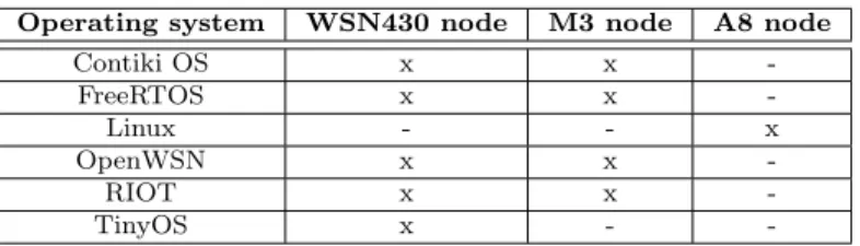
Operating system WSN430 node M3 node A8 node
Contiki OS x x -FreeRTOS x x -Linux - - x OpenWSN x x -RIOT x x -TinyOS x -
-Table 2: IoT operating systems supported by the FIT IoT-LAB platform. Defining complementary and heterogeneous testbeds with different node types, topologies and environments allows for coverage of a wide range of real-life use-cases, and thus, researchers may expect different behaviors from each platform.
3.2. Testbed access and policy
The platform can be accessed through the web portal or using provided command-line tools. In addition, the platform offers a hosted environment on SSH front-ends, featuring pre-installed CLI Tools, target architectures cross-compiler toolchains, experiments results, and access to devices serial ports. It is also possible to use a dedicated xubuntu virtual-machine on a Linux/Mac/Windows workstation based on virtual-box. The overall archi-tecture of the IoT-LAB testbed is depicted on Figure 3.
The IoT-LAB nodes can be entirely reprogrammed, depending on the needs of each user. Remote users can flash any firmware they want, using any embedded operating system (e.g., TinyOS, Contiki OS, RIOT). Currently, five popular loT operating systems are supported (see Table 2).
For instance, in order to implement a new routing protocol, a user needs to choose an operating system first. Depending the chosen system, the new functionality could be implemented as a library or directly inside the main program. The IoT-LAB testbed provides all necessary drivers, librairies and application templates in order to start developing a new protocol for the
major operating systems in this research field2.
Once registered, any remote user can use some nodes for the needs of his experiments. The IoT-LAB testbed tools allow to create and submit an experiment, and then to interact with running nodes. Users first select the nodes they want to use. A map of each site is available, showing both the physical topology and the identifiers of nodes. Once booked, the nodes can be set up with any firmware file. Once deployed, the experiment can start. During the experiment, the SSH front-end enables interaction with the firmware running on the nodes (e.g., reading sensor values, sending radio packets).
Finally, the testbed is open in three different ways:
• political side: IoT-LAB is opened to everyone (e.g., academic, indus-trial, students). An account can be created by filling up a motivation
form through the website3;
• financial side: IoT-LAB is free to use, no billing being performed; • technical side: there is no limitation with the code people upload to the
nodes. We also allow users to send custom nodes in order to evaluate new hardware.
3.3. ICube’s platform
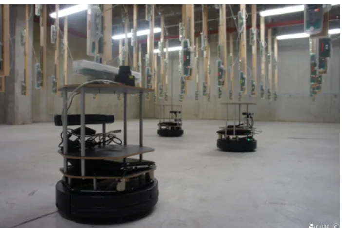
In this investigation we focus on the site of ICube Strasbourg. ICube’s platform offers two testbeds; the one is structured as a 3D grid with 10 lines and 8 columns, distributed in three layers of 80 nodes each, thus, in total 240 fixed WSN430 nodes, while the other testbed consists of 64 M3 and 14 A8 nodes respectively, distributed in two layer of 39 each. Furthermore, ICube offers 44 mobile nodes, 7 WSN430 and 37 M3 based-boards respectively (see Figure 4).
2
https://www.iot-lab.info/dev-center 3
Figure 4: A view of ICube’s platform.
Considering various technical constraints such as autonomous navigation with a certain minimal speed, carrying and powering an IoT-LAB node (with
size of 32× 8 × 6 cm), automatic docking, at least three hours of battery
autonomy and realtime monitoring of the robot, drove the engineers of
IoT-LAB to TurtleBot24 robots where Robot Operating System (ROS5)
frame-work (e.g., navigation stack with the AMCL module) is used. TurtleBot2 is able to replay trajectories with a list of checkpoints. Indeed, the users may choose among the predefined trajectories or design their own circuit to perform their experiments. The robots move with speed of 30cm/sec and may communicate both with static nodes and other mobile nodes. Finally, each TurtleBot2 has a dedicated docking station for charging and reserving purposes.
Even though the open testbed is very complete, still in the following section, we will present through a number of experimental campaigns that it misses some important guidelines and features, and to show how to retrieve scientific and meaningful results instead of proofs-of-concept only, by utilizing a not complex set of code.
4http://www.turtlebot.com/ 5http://www.ros.org/
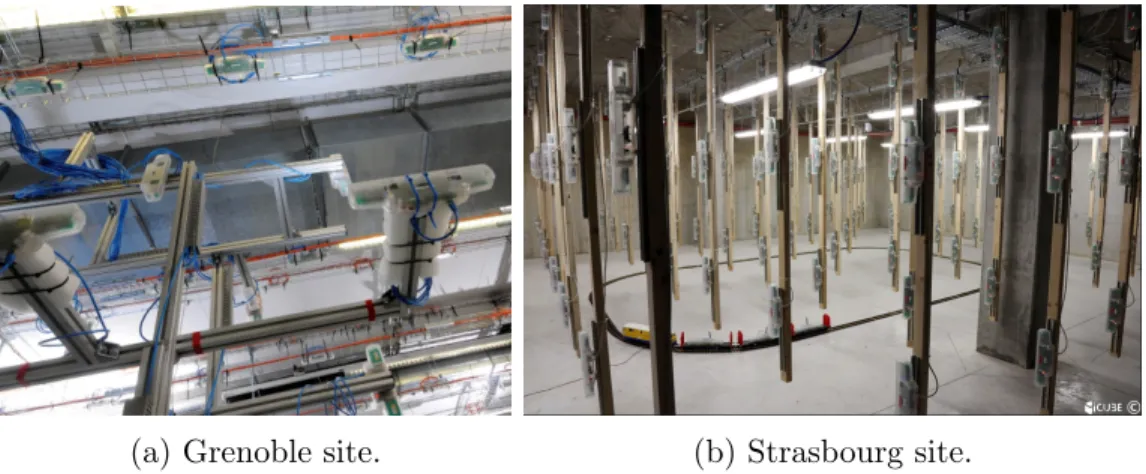
(a) Grenoble site. (b) Strasbourg site.
Figure 5: A variety of radio environments with two of the seven deployment sites of the FIT IoT-LAB testbed.
0 10 20 30 40 50 60 70 Width (m) −10 0 10 20 30 Le ng th (m )
(a) Grenoble site.
−5 0 5 10 15 20 Width (m) 0 5 10 Le ng th (m ) (b) Strasbourg site.
Figure 6: Different testbed topologies with M3 nodes on FIT IoT-LAB .
4. Thorough analysis of an IoT testbed
In this section we present our thorough experimental study over the testbed located in ICube Strasbourg. This testbed belongs to the half real-world testbed category. Standing inside a dedicated room (without shielded walls), Strasbourg nodes remain subjected to external interferences with wire-less devices using other technologies, such as Wi-Fi (2.4 GHz band) and GSM (868 M Hz band). Note that site selection plays a major role in experiments since all sites of the FIT IoT-LAB testbed were made different on purpose.
The primary goal was to propose a variety of physical topologies and hardware. Each site also presents its own radio characteristics, in terms of radio environments and surrounding wireless devices. For instance, we here observe that nodes of Strasbourg form a regular 3D grid in a dedicated room while the ones of Grenoble were spread throughout a real-world environment (i.e., non isolated room hosting various hardware for robotics). Therefore, the observed performances of a given protocol may vary from one site to another (e.g., MAC layer as medium access performances greatly depend on radio environment). Figure 6 illustrates two of the seven deployment sites, i.e., Grenoble and Strasbourg.
The limited geographical scope of those indoor testbeds may prevent some users from experimenting solutions at the scale of much larger environments (e.g., forest, city). Scenarios requiring such dimensions could be evaluated by adapting communication ranges and distances in order to reach a small-scale
model city or forest (e.g., Strasbourg’s site already providing a 360m2 room).
Adjustment of transmission ranges would allow to reach such goal. Ongoing works in the FIT IoT-LAB platform also focus on noise injection controlled by users. Even though anticipating the impact of this physical phenomenon is far from being trivial, it could be used to degrade the quality of com-munications and thus force nodes to use more hops to reach a destination. Furthermore, on the software side, some physically neighboring nodes could be eliminated from the logical neighborhood. Such a virtual neighborhood would then consist into nodes with which communication link quality (e.g., RSSI, LQI, PRR) is above a given threshold. Note that the largest site of
FIT IoT-LAB, Grenoble, also allows experiments in a 60m× 40m area where
the longest distance between two sensors reaches nearly 110 meters. Future works regarding FIT- IoT-LAB also include the possibility for users to launch experiments simultaneously over multiple sites. So far, nodes from two dis-tinct sites can not communicate but such a feature could be envisioned. Two nodes located in two distant facilities (e.g., Lille and Strasbourg, 500km be-tween both) would be allowed to communicate through the classical Internet architecture while the testbed would emulate a radio link on top of it. In other words, emulated communications would be affected as if they had hap-pened under wireless assumptions (e.g., asymmetry, interferences, losses).
In our set of experiments, we chose the 80 nodes of the middle layer to work on our study. All 80 nodes are randomly selected as data sources and implement a time-driven application model by broadcasting in Constant Bit Rate (CBR) mode one packet every 60 seconds. We chose a 10 bytes
Topology parameters Value
Testbed organization Regular grid (10 m× 8 m × 3 m)
Deployed nodes 80 fixed sensors (1 meter of node spacing)
Experiment parameters Value
Duration 150 min
Application model Time-driven: CBR 1 pkt/min
Type of Transmission Broadcast
Number of events 7900 pkts
Payload size 10 bytes (+ 6 bytes MAC header)
MAC model X-MAC [28]
Sampling frequency (125, 250, 500) ms
Maximum retries 3
Hardware parameters Value
Antenna model Omnidirectional CC1101
Radio propagation 868 M Hz
Modulation model GFSK
Transmission power (−10, −15, −20, −25, −30) dBm
Battery 880 mAh, 3.7 V
Table 3: Experimental setup.
data size, which corresponds to the general information used by monitoring applications (e.g., node ID, packet sequence, sensed value) [9]. We run a number of experiments by considering different transmission power values
(i.e., −10 dBm to −30 dBm) in order to study the impact of the radio
model in transmission range and link quality. The experiments lasted for 150 minutes while 7900 transmissions occurred in each round.
In this campaign, we aimed at removing assumptions one at a time. Thus, we performed our evaluation within an idealistic scenario where we kept our application as simple as possible, while no routing protocol is running in the network. As a result, this scenario allowed us to focus on the performance of the open testbed by affecting the results at minimum. Furthermore, at the MAC layer, we employed X-MAC [28] protocol with sampling frequencies at 125 ms, 250 ms and 500 ms. Among all supported operating systems (e.g., TinyOS, OpenWSN), we implemented our project on top of the Contiki OS [29]. The details of the experimental setup are exposed in Table 3.
Hereafter, we detail the results obtained from our experimentations (i.e., neighbourhood density and stability, quality of the radio links, energy con-sumption, drifts over predefined trajectories).
-30 -25 -20 -15 -10 Transmission power (dBm) 0 5 10 15 20 25 30 35 40 N um be ro fn ei gh bo rs
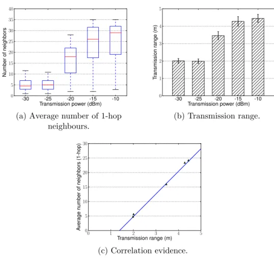
(a) Average number of 1-hop neighbours. -30 -25 -20 -15 -10 Transmission power (dBm) 0 1 2 3 4 5 Tr an sm is si on ra ng e (m ) (b) Transmission range. 0 1 2 3 4 5 Transmission range (m) 0 5 10 15 20 25 30 A ve ra ge nu m be ro fn ei gh bo rs (1 -h op ) (c) Correlation evidence.
Figure 7: Neighbourhood density (left), transmission range (center) and the correlation between both (right).
4.1. Selecting the transmission power
To estimate the density in the network, we count the average number of neighbours per node. To do so, we calculate the successful symmetrical packet transmissions among the nodes for various transmission power values
(i.e., from−10 dBm to −30 dBm). In order to perform a fair analysis, in our
campaign, we kept the high-quality symmetrical links (i.e., over than 90% of successful receptions in both ways), with confidence intervals below 10%. In Figure 7a, the average number of neighbours per transmission power is de-picted. As expected, the higher the transmission power, the more neighbours a node has, and consequently higher the density in the network. It is worth
to point out that the pairs (−30, − 25) dBm, and (−15, − 10) dBm present similar results. In order to better comprehend this behaviour, by employ-ing the Euclidian distance equation, we studied the correlation between the transmission range and the transmission power. As can be observed from Fig-ure 7b, the transmission range follows similar trend with the neighbourhood density. Moreover, unlike most radio propagation models used in simulation, the transmission power is not linearly reflected in the transmission range. In this context, using a realistic environment helps researchers getting closer to real deployments, in a way that cannot be obtained through simulations.
To better understand the previously obtained results, we studied the cor-relation between the transmission range and the average number of 1-hop neighbours. We first used a scatter plot (see Figure 7c) that demonstrates a linear correlation between the two distributions. Indeed, we obtained a linear correlation coefficient of 0.98. We then used the least squares fitting method,
and extracted the following relation: f (x) = −10.8 + 7.8x with x being the
transmission range and f (x) the resulting average of 1-hop neighbours (see the blue curve in Figure 7c). Although the increase of transmission power is not directly linearly reflected in the transmission range (but rather by several linear stages), this simple relation seems to remain quite robust despite the experimental noises.
4.2. Characterizing wireless links of a testbed
There are certain situations that neither occur in simulations nor in ex-perimental deployments when employing only few nodes. Among those, the presence of links with bad quality induces packet losses, and therefore, may introduce a bias in the statistical measurements. Hence, in realistic deploy-ments researchers should take into account that most of the communication links are unstable, unreliable or even unidirectional.
4.2.1. Assessing link quality and stability
However, most of routing and MAC protocols require bidirectional links so that two nodes can exchange information (e.g., data, acknowledgements), thus, it is essential to evaluate wether this assumption can be preserved in testbeds. We therefore aimed at providing a comprehensive analysis of the link quality in a testbed.
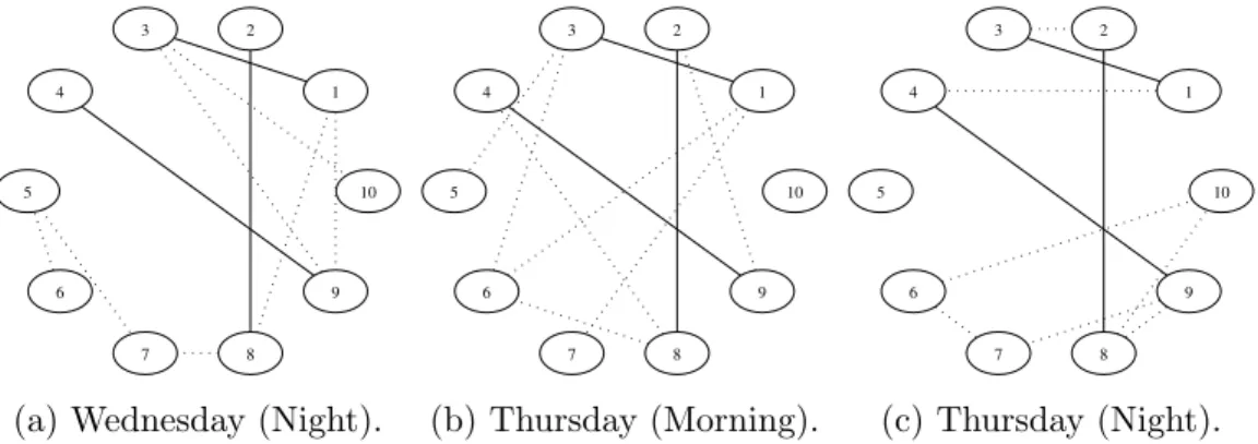
1 3 9 2 10 4 5 7 6 8
(a) Wednesday (Night).
1 3 7 2 5 4 6 8 9 10 (b) Thursday (Morning). 1 3 4 2 5 6 7 10 8 9 (c) Thursday (Night).
Figure 8: Links stability over time.
Several criterions may be considered to represent and evaluate the link quality and stability. We, first measured the PRR of each link, along with their bidirectionality, in the testbed by configuring each node broadcasting in turn 100 data packets and computing the number of subsequent receptions. Thus, we were able to precisely compute the PRR of each link as well as its bidirectionality. In this scenario, we considered a transmission power of −20 dBm, and evaluated the stability of links over time. In particular, we repeated this experiment three times every 12 hours, once on Wednesday evening and twice on Thursday (morning and evening respectively). Then, we analyzed the links properties in order to study their stability over time. In Figure 8, the nodes are depicted in a circle for visualization purpose. Ten nodes are a subset of the total 80 nodes. As it can be observed, three connected components (little more than 30% of the links) remain stable over time (links 1-3, 2-8 and 4-9, plain arrows) while variations occur among the remaining links (dotted arrows).
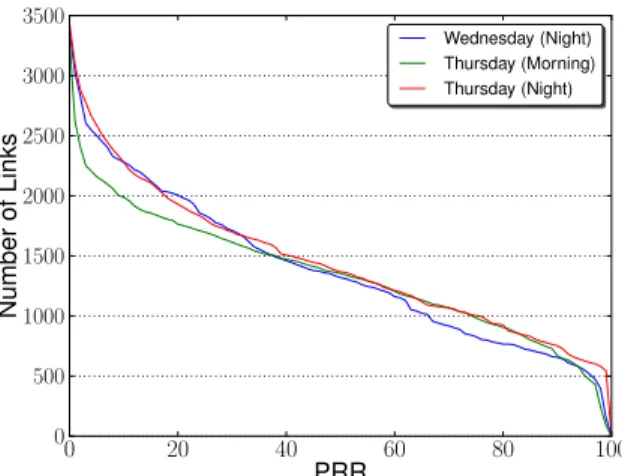
As previously mentioned, in real deployments the link quality and sym-metry may significantly vary over time. Figure 9 displays a detailed repre-sentation of link quality throughout the whole experimental procedure, in particular the total number of bidirectional links per PRR is presented. The results show that all three experiments follow similar trend. In fact, more than 500 bidirectional links present PRR above 90%. However, this behavior is very hard to reproduce in simulators. Thus, researchers often need to re-move this assumption, while preserving identical density over time (in order to perform a meaningful evaluation).
As it is presented in Table 4, ICube platform preserves certain stability in terms of network density, (i.e., approximately 14 neighbours) with PRR
0 20 40 60 80 100 PRR 0 500 1000 1500 2000 2500 3000 3500 N um be ro fL in ks Wednesday (Night) Thursday (Morning) Thursday (Night)
Figure 9: Links quality over time.
Date Neighbours Confidence Interval
Wednesday (night) 13.95 2.16
Thursday (morning) 13.38 1.9
Thursday (night) 15.34 1.94
Table 4: Average number of 1-hop neighbours over time.
above 90% in all three experiments. Then, the density criterion remains stable while the links are changing. Thus, it allows researchers to remove assumptions one at a time, to better evaluate their protocols. It also shows that the testbed can be used either way. Indeed, it can be used as a scientific tool, producing scientific results that can be reproduced and slightly vary over time, even with a changing topology of identical density. When enlarging the set of considered links for experimentation, users would introduce more and more randomness due to the lower quality of those links, thus reaching real life conditions and meeting some of the requirements for the validation of a proof-of-concept and iterative prototyping.
In our experiments, each node was transmitting sequentially, and thus, no potential collision due to simultaneous transmissions was experienced during the experiments. To further explain the PRR performance in our experi-mental evaluation, we investigated more powerful nodes (M3), other anten-nas (2.4GHz) and another operating systems (custom firmware). We kept obtaining unstable performances regarding the PRR metric. Several reasons may explain this instability:
Topology parameters Value
Testbed organization Regular grid (16 m× 8 m × 3 m) Deployed nodes 31 fixed FIT IoT-LAB M3 nodes
Node spacing Two meters
Experiment parameters Value
Duration 60 min
Application model Event-driven: 100 pkts/burst Type of Transmission Broadcast
Number of events 93000 pkts
Payload size 40 bytes (10bytes header)
MAC model Not available
Burst frequency 10 ms
Hardware parameters Value
Antenna model Omnidirectional
Radio propagation 2.4 GHz
802.15.4 Channels 11 to 25
Modulation model AT86RF231 O-QPSK
Transmission power +3 dBm
Table 5: Experimental setup.
1. Channel randomness at each node: all our Figures (i.e., 6a, 6b, 7, 9 and the new 10 with M3 hardware) demonstrate the dynamic behavior of the links among the nodes.
2. No retransmission: it is important to note that the nodes were trans-mitting in broadcast, which indicates that there are no retransmissions in case the data packet is not received.
3. Potential interferences: we ran experiments on the second layer (i.e., 80 nodes) during several days. Since there is always probability that there are ongoing experiments concurrently, from other researchers. 4. Other surrounding networks: last but not least, since our testbed
con-tains some WiFi access points, poor packet reception rates could also be due to WiFi beaconing and traffic, as observed on Grenoble’s site [30]. Therefore, researchers running experiments should be aware of which topologies they could use for reproducible setups (e.g., stable with good links) and the ones they should keep for proof-of-concepts only (e.g., lossy and unstable links over time).
Width (m) −2 0 2 4 6 8 10 12 14 16 Leng h (m ) 0 2 4 6 8 PDR (% ) 75 80 85 90 95 100 A B C Wi-Fi ch 11 ch 12 ch 13 ch 14 ch 15 ch 16 ch 17 ch 18 ch 19 ch 20 ch 21 ch 22 ch 23 ch 24 ch 25 56 54 42 50 60 62 64 32 24 26 20 22 46 28 40 2 4 6 8 34 12 14 10 38 58 16 18 30 36 52 48
(a) Day 1 (afternoon).
Width (m) −2 0 2 4 6 8 10 12 14 16 Leng h (m ) 0 2 4 6 8 PDR (%) 75 80 85 90 95 100 A B C Wi-Fi ch 11 ch 12 ch 13 ch 14 ch 15 ch 16 ch 17 ch 18 ch 19 ch 20 ch 21 ch 22 ch 23 ch 24 ch 25 56 54 42 50 60 62 64 32 24 26 20 22 46 28 40 2 4 6 8 34 12 14 10 38 58 16 18 30 36 52 48 (b) Day 2 (morning). Width (m) −2 0 2 4 6 8 10 12 14 16 Leng h (m ) 0 2 4 6 8 PDR (%) 75 80 85 90 95 100 A B C Wi-Fi ch 11 ch 12 ch 13 ch 14 ch 15 ch 16 ch 17 ch 18 ch 19 ch 20 ch 21 ch 22 ch 23 ch 24 ch 25 56 54 42 50 60 62 64 32 24 26 20 22 46 28 40 2 4 6 8 34 12 14 10 38 58 16 18 30 36 52 48 (c) Day 3 (night).
Figure 10: PRR reproducibility over three different experiments: interference “free” scenario (Wi-Fi beacons are transmitted).
4.2.2. Reproducing wireless topologies
For this study, we used 31 M3 nodes of the second upper layer of the
Strasbourg testbed6), all of them being sequentially selected as data sources
and implementing a burst-driven application model. Each was broadcasting 100 packets in a row with interval of 10 ms, at +3 dBm transmission power. We chose a 40 bytes data size, which corresponds to the general information used by monitoring applications [9]. We performed a thorough analysis of the radio links by iterating experiments over all IEEE 802.15.4 channels from 11 to 25. Each experiment lasted for 60 minutes and was repeated seven times over different time periods (i.e., morning, afternoon, evening and night). The details of this experimental setup are exposed in Table 5.
Figures 10, 11 and 12 depict the obtained results from this experimental campaign. Figure 10 shows the PRR averages of the different 802.15.4 chan-nels that were observed at three distinct days and different periods of time. Overall, observed channels presented stable performances in terms of PRR. Only few channels (e.g., 17, 18) exhibited some important changes on day 3, thus, endangering the reproducibility of a setup using this channel and being tested during these three periods.
For the sake of clarity, Figure 11 exhibits only the links that we con-sidered to be of good quality. We concon-sidered good and bidirectional links where the PRR was above 90% on all 802.14.5 channels. Here again, we can observe that even good links vary over time with more or less of them being
6We used a custom firmware provided by the FIT IoT-LAB [31]:
Width (m)6 4 2 0 8 10 12 14 16 Length (m ) 0 1 2 3 4 5 6 7 8 Heigt h ( m) 1.95 2.00 2.05 2.10 2.15 2.20 2.25 56 54 42 50 60 62 64 32 24 26 20 22 46 28 40 2 4 6 8 34 12 14 10 38 58 16 18 36 30 52 48
(a) Day 1 (afternoon).
Width (m)6 4 2 0 8 10 12 14 16 Length (m ) 0 1 2 3 4 5 6 7 8 He igt h ( m) 1.95 2.00 2.05 2.10 2.15 2.20 2.25 56 54 42 50 60 62 64 32 24 26 20 22 46 28 40 2 4 6 8 34 12 14 10 38 58 16 18 36 30 52 48 (b) Day 2 (morning). Width (m)6 4 2 0 8 10 12 14 16 Length (m ) 0 1 2 3 4 5 6 7 8 He igt h (m) 1.95 2.00 2.05 2.10 2.15 2.20 2.25 56 54 42 50 60 62 64 32 24 26 20 22 46 28 40 2 4 6 8 34 12 14 10 38 58 16 18 36 30 52 48 (c) Day 3 (night).
Figure 11: Analysis of Good Links (in green), bidirectional PRR is over 90% for all 802.15.4 channels, and Stable Good Links (in red), bidirectional PRR is over 90% for all
802.15.4 channels in all experiments of three days.
Day1 1pm (a)
Day1 4pmDay1 12pmDay2 8am (b) Day2 5pmDay3 1am (c)Day3 10am Experiments 0 100 200 300 400 500 Nb Li nk s
Stable Good links
Good links Unbalanced linksBad links
Figure 12: Stable Good, Good and Unbalanced links over 7 different experiments in three different days.
available at different time periods. That would mean that naive solutions for reproducibility (i.e., keeping only good links) would fail in such situations.
Finally, Figure 12 summarizes those results by showing the evolution of the distribution of radio link quality over time. We can observe that there are very few stable and good links, thus, much reducing the number of available topologies one could pick up for getting reproducible experiments. Moreover,
Average RSSI
PR
R
(a) Correlation between RSSI and PRR.
Average LQI
PR
R
(b) Correlation between LQI and PRR.
Figure 13: Interest of RSSI and LQI values to evaluate link quality and symmetry.
even though the quantities of bad, unbalanced, good, and stable good links do not vary much over time, the links themselves may not be the same from one period to another (see Figure 11).
Therefore, reproducing results may not be achieved by simply repeating experiments with identical setups [32]. People running experiments should be assisted by some dedicated tools to help them characterize the used topologies and their associated trust level. This latest would allow people to select the most appropriate nodes and links for testing their own solutions and comparing the obtained results to the existing ones.
4.3. Selecting the quality radio links
As previously mentioned, many protocols throughout the communication stack require bidirectional links to operate. While this assumption can be guaranteed in simulation, it does not stand in experimental conditions. Con-sequently, researchers often need to keep only a set of stable, high-quality and bidirectional links to evaluate their solutions.
Most radio chipsets provide indicators that could be used for this purpose, such as the RSSI, expressed in dBm, and the LQI. The RSSI value is an estimate of the signal power level in the radio channel while the LQI estimates how easily a received signal can be demodulated. Therefore, we studied those metrics in order to characterize radio links. As depicted in Figure 13, the RSSI can hardly help estimate the PRR of a link, as there is no strict relation
PRR spanning from 0% to 80%). A similar conclusion can be drawn for the LQI value. However, the RSSI can help to select a set of high-quality links.
Indeed, links with a RSSI abobe −83 dBm all display a PRR greater than
90%. The LQI, however, can not ensure the same guarantee. 4.4. Evaluating the energy consumption
Simulators provide an estimation of the energy consumption of sensor nodes. Indeed, they often provide a linear model, where all nodes follow
a similar and often predictable energy consumption patterns. Moreover,
they consider a subset of energy consumption causes only (e.g., transmission, CPU). On the contrary, in reality two identical nodes may follow different consumption patterns, and some minor changes in the protocol configura-tion may present unexpected impact. In this set of experiments, we demon-strate how the consumed energy can be accurately and efficiently retrieved in open testbed. To this aim, we considered the example of X-MAC protocol with various sampling frequency configurations, 125 ms, 250 ms and 500 ms (i.e., X-MAC125, X-MAC250 and X-MAC500 respectively). We configured the nodes to constantly sample the medium while decreasing their sampling frequency every 100 seconds, from 125ms to 500ms. Note that no packet transmissions took place in this campaign.
Figure 14a presents an accurate energy consumption for two distinct nodes and average for the whole network.
100 150 200 250 300 350 400 Experimentation time (s) 10.0 10.5 11.0 11.5 12.0 12.5 13.0 13.5 14.0 En erg y c on su mp tio n ( mW ) X-MAC125 X-MAC250 X-MAC500
Average of all nodes Node 106 Node 88
(a) Real time energy consumption.
Width (m) 1 2 3 4 5 6 7 8 Length (m) 1 234 5678 910 Total energ y con sume d (W) 35 40 45 50 55
(b) Total energy consumption in 3D representation.
Figure 14: The average (left) and total (right) energy consumption in various sampling frequency configurations.
Overall, there is some difference (i.e., close to 0.5 mW ) among the nodes, although equipped with identical hardware components. It is worth to point out that energy profiles can be first established. Then, the end user could choose either homogeneous or heterogeneous nodes, depending on the studied scenario.
We also performed a mapping of the energy depletion throughout the net-work, in order to identify its repartition and disparity among the nodes. To do so, we measured the total energy consumption of each node for the total duration of the experiments. The results of this evaluation are displayed in Figure 14b, which depicts our deployment room (x and y axises) and the energy consumption at each node (z axis). Looking more closely, the nodes present differences in energy consumption (i.e., from 35 W to 50 W ), while distinct simulations using the same setup would have nodes with homoge-neous behaviour. This anomaly brings us a step closer to real deployments where the researchers may have to deal with plethora of unexpected be-haviours. As a result, it can be seen as an advantage for testbeds compared to simulators, as they allow us to get a flavor of real-world deployments. 4.5. Assigning and planning trajectories for mobile robots
Most IoT testbeds present static topologies that allow the evaluation of a large variety of scenarios. FIT IoT-LAB testbed was built as an original tool for an in-depth understanding of the experimental factors that may affect the performance of any WSN. Among the large variety of operated deployments back then, very few were standing out and trying to involve mobile sensor. An increasing number of contemplated scenarios now involve more mobile sensor nodes in multi-hop topologies, while expecting to last months or even years. However, very little is known today about mobility and almost no testbed is available to design and check new solutions against a real environment. In order to allow our research community to benefit from a dedicated tool that enables large scale experimentations on mobile WSN, our prime objective was to set up a large number of mobile nodes. That had to come along advanced mobility patterns in order to attract multiple types of users. Nodes were expected to move either according to pre-defined trajectories or based on pre-computed paths reflecting a random mobility model or also along replayed movement traces.
However such an implementation should allow for repeatability of tra-jectories (e.g., paths, speed). The preliminary testbed (SensLAB) had four wireless nodes embedded on an electric train. Trajectory was determined by
the static rail circuit while nodes were powered by the rails [33]. Indeed, the static circuit could have been changed but that would have required a physical intervention for each new configuration, which was not realistic in terms of operating costs and manpower.
Eventually, we aimed at a more flexible solution. We started with some landmarks on the floor in order to identify the mobility scenario. That was considered as too limiting, again because of the mandatory ability for any user to change trajectory, which would have forced testbed operators to upgrade landmarks for any new path.
We therefore deployed RFID tags on a grid topology (with a 50 cm step), all over the floor. Mobile nodes were equipped with a RFID reader and any trajectory would have been implemented as a set of RFID identifiers, assum-ing that mobile nodes had embedded a map of all spread RFID tags of the room. This solution did not provide satisfactory results (e.g., heavy energy consumption, fixed granularity of the trajectories, potential collisions be-tween mobile nodes). Indeed, all trajectories should have been cross-checked in order to ensure that no collision would occur, and if it were, enhanced conflict resolution between antagonist paths should have been studied.
Consequently, we opted for the use of cameras and range detector sensors on each mobile robot. The 3D camera appeared as the best value positioning system for our robots. Technically, it can work autonomously without an external server or anchors. 3D Camera is based on infrared beam projection which can evaluate obstacles range. This range detection is used by the navigation program running on the robot netbook in order to compute the position. It also offers collision avoidance while detecting other robots.
We therefore, in this subsection, investigate the ability of robots to accu-rately follow the predefined trajectories that are available to the users. More specifically, we aim on showing the drifts that the robots may present due to the potential miscalculation of the navigation system. Hence, for this cam-paign we utilized two TurtleBot2 robots. This model was chosen for many reasons, ranging from the affordable cost of a robot to its evolution capaci-ties. Our prime objective was to be able to control those mobile nodes with some built-in robotics mechanisms and an operating system we could make cooperate with the systems envisioned on the embedded sensors.
We set the robots to replay over a line (from point A to B and vice versa) and square (A, B, C and D coordinates) trajectories for 90 minutes to obtain a large set of data related to the coordinates of the robots (ten samples per second). To calculate the robot’s drift, we first determine the equation
0 2 4 6 8 10 12 X axis (m) −2 0 2 4 6 8 10 12 Y ax is (m ) A B
(a) Line trajectory with roundtrips.
−4 −2 0 2 4 6 8 X axis (m) −2 0 2 4 6 8 10 12 Y ax is (m ) A B C D (b) Square trajectory.
Figure 15: Robot’s drifts over predefined trajectories, Y axis indicates the length while the X axis the width of the room, respectively.
of the line ε (i.e., −→AB) (1), considering the given coordinates, A1(x1, y1) and
B2(x2, y2) for instance. We then, calculate the distance d(M0, ε) (2), between
position M0(x0, y0), position of the robot, and the line ε.
ε = Ax + By + Γ (1)
d(M0, ε) = |Ax
0+ By0 + Γ|
√
A2+ B2 (2)
In Figures 15a and 15b the drifts of the mobile robots with respect to the predefined circuits (i.e., line and square) are illustrated. As can be observed, the robots replay the line trajectory with a drift of 0.57 m while the square circuit with 0.46 m in average. The detailed results are presented in Table 6. Such drifts should not be neglected regarding the transmission ranges that we have. Not only do they endanger repeatability of trajectories of mo-bile nodes, they may also change the overall connectivity between wireless sensors. Indeed, as already discussed, our transmission radio range from 2 to 5 meters approximately (see Figure 7b). Therefore, a 0.5 m drift rep-resents a difference ranging from 10 to 25%, thus potentially changing the communication topology. More specifically, the accuracy of the evaluation of some mechanisms aimed at mobility management would be impacted by such drifts (e.g., handover procedures [34]).
Drift AVG 5 PCTL Median 95 PCTL CI
Line (m) 0.576 0.018 0.342 1.856 0.005
Square (m) 0.469 0.013 0.248 1.406 0.004
Table 6: Trajectory drift measurements
hardware respectively. On the one hand, the AMCL module, the navigation stack of the ROS framework, computes the robots path in order to smooth the trajectories, as a result, the recorded traces are not in line with the predefined checkpoints-based trajectories. We are currently adjusting both the navigation stack and the smoothing algorithm in order to leverage this effect. On the other, as can be observed, the mobile robot presents a slight drift among its loops over the very same circuit. This hardware-related drift is introduced due to the sensors odometry that employed by the navigation system of TurtleBot2. However, the 3D camera (with the range detector sensor) that should handle the odometry drift, lacks in open-space and large-scale environments where not enough landmarks exist to compute the path. In fact, the maximum distance that the 3D camera may reach is 8 meters, thus, we observed that in certain positions the robot is too far from the wall (i.e., the landmark). Note that the dimensions of Strasbourg site is 10 to 12 m. We, thus, assume that the robots may present a better behaviour in corridor-based scenarios e.g., Grenoble site.
As a result, the miscomputation of the AMCL navigation in conjunction with the sensors odometry navigation may explain the drifts of the mobile robots in our experiments. This phenomenon appears to be to the detriment of mobile robots that carry wireless sensor nodes, thus, raising the question of cost versus accuracy versus quantity of robots in our community.
Currently, we implement and deploy only one mobility model for the robots based on predefined path with checkpoints. Our future developments will allow users to draw their own predefined paths.
Overall, we aimed at showing that various hardware and environment parameters can be controlled and kept stable over multiple instances of a same experimentation setup (e.g., node radio coverage, trajectories of mo-bile robots). Open testbeds therefore allow researchers to face real-world conditions while guaranteeing the scientific nature of their observations and results. On the contrary, the simulators by employing mobility plug-ins, such
Simulation Experimentation
Radio links • high-level reproducibility • low-level reproducibility overall
(high-level for high-quality links only)
• theoretical models • real-world radio environment
Network topology • high-level reproducibility • low-level reproducibility
(most of links being of mid or low quality)
Node mobility • high-level reproducibility • mid-level reproducibility
(drifts being induced)
Energy consumption • mid-level accuracy • high-level accuracy
Table 7: Simulations and experiments: complementary approaches for validation of WSN and IoT solutions.
as BonnMotion7, allow the mobile nodes to follow and reproduce accurately
the predefined trajectories without imposing drifts in their traces. 5. Further Discussions
Performance analysis of newly designed algorithms and protocols is ex-tremely desirable for efficient IoT and WSNs deployments. Simulation and experimental evaluation methods are essential steps for the development pro-cess of protocols and applications. Nowadays, the new solutions can be tested at a very large scale over both simulators and testbeds. On the one hand, simulators and emulators allow researchers to isolate or simplify some as-sumptions (e.g., radio propagation) by tuning configurable parameters to serve proof-of-concept requirements. Therefore, simulation is more suitable for evaluating and comparing the solution with its competitors from the state-of-the-art. On the other, a testbed is a platform for experimentation which allows for rigorous and transparent evaluation of new protocols, and reflects some potential anomalies that their proposal may show later. Testbeds and simulators are two crucial and complementary design and validation tools for achieving a successful real-world deployment (see Table 7).
Theoretically, development process should start from the theoretical anal-ysis by providing bounds and indication of its performance to be validated and verified by simulations and finally confirmed in open testbeds.
Our objective was to discuss to what extent results obtained from exper-iments could be considered as scientific, i.e., reproducible by the community. In this article, we did not focus on simulators against testbeds. Our prime goal was to translate good simulation practices into experimentation guide-lines. Indeed, similar results should be obtained by anyone having access
to the same simulator, with the same proposed solution and the same com-plete simulation setup. Enhanced characterization of testbeds made available to the community should pave the way towards more scientific results from these facilities. Undoubtedly, simulators will also move forward and integrate better models and tools to allow for always improved realism (e.g., appear-ance/disappearance of wireless links). They should also remain the logically preferred tool for mobility investigations as they are able to integrate differ-ent kinds of settings (e.g., hardware variations, antenna variations, speed of mobile robots), which remain static and less prone to evolve in real testbeds. Hence, once the entire performance evaluation procedure is successfully done and the results present coherence, then researchers could push their solutions to engineers in order to proceed with real-world deployments. As a result, the researchers lower the entry cost and extra management burden to real-world experimentation, which often considered as a complex, time-consuming and heavyweight activity, to accelerate proof-of-concept evalua-tion and competitiveness.
6. Conclusions and Perspectives
In this paper, we observed the constantly growing importance of experi-mentations in our research domain. Our objective was to identify what value such platforms could add to WSN and IoT protocol evaluation, and how they could be efficiently and successfully coupled with simulations.
We investigated the node radio coverage based on the transmission power, as a result, allowing users to select the most suitable transmission power for their experiments. Moreover, we exposed how both real time and total en-ergy consumption can be accurately monitored, and to what extent the link quality and stability assumptions can be removed or not, at the researchers choice. Furthermore, we presented the accuracy of the robots to replay the predefined trajectories. Hence, the evaluation campaign of WSN protocols can go one step further towards real-world deployment by removing the previ-ously mentioned assumptions, at little time cost and with limited complexity. Finally, we studied whether the studied experimental setup is repeatable and, moreover, whether the obtained performance evaluation results are re-producible by the community. Indeed, such open facilities allow researchers to run multiple instances of a same experimental setup over stable and finely controlled components of hardware and real-world environment.
Our ongoing and future work consists of further exploring the role of testbeds in the development procedure of protocols and applications. We
would like to investigate the impact of the transmission power in the con-struction of the network topology. Especially, we would like to allow testbed users to accurately anticipate the physical network topology, upon sole knowl-edge of transmission power assigned to each node. Furthermore, we plan to further study and optimize the localization, orientation and navigation stack of ROS, and to introduce landmarks inside the open testbed in order to evaluate the accuracy of the mobile robots.
References
[1] V. Dyo, S. A. Ellwood, D. W. Macdonald, A. Markham, C. Mascolo,
B. P´asztor, S. Scellato, N. Trigoni, R. Wohlers, and K. Yousef,
“Evo-lution and Sustainability of a Wildlife Monitoring Sensor Network,” in Proceedings of the 8th ACM Conference on Embedded Networked Sensor Systems (Sensys), 2010, pp. 127–140.
[2] M. Li and Y. Liu, “Underground Structure Monitoring with Wireless Sensor Networks,” in Proceedings of the 6th ACM/IEEE International Conference on Information Processing in Sensor Networks (IPSN), 2007, pp. 69–78.
[3] O. Chipara, C. Lu, T. Bailey, and G. Roman, “Reliable Clinical Mon-itoring using Wireless Sensor Networks: Experiences in a Step-down Hospital Unit,” in Proceedings of the 8th ACM Conference on Embedded Networked Sensor Systems (Sensys), 2010, pp. 155–168.
[4] K. Langendoen, A. Baggio, and O. Visser, “Murphy Loves Potatoes: Experiences from a Pilot Sensor Network Deployment in Precision Agri-culture,” in Proceedings of the 20th IEEE International Symposium on Parallel and Distributed Processing (IPDPS), 2006, pp. 174–174.
[5] J. Kropf, L. Roedl, and A. Hochgatterer, “A modular and flexible system for activity recognition and smart home control based on nonobtrusive sensors,” in Proceedings of the 6th International Conference on Perva-sive Computing Technologies for Healthcare (PervaPerva-siveHealth), 2012, pp. 245–251.
[6] G. Chelius, C. Braillon, M. Pasquier, N. Horvais, R. Gibollet, B. Es-piau, and C. Coste, “A Wearable Sensor Network for Gait Analysis:
A Six-Day Experiment of Running Through the Desert,” IEEE/ASME Transactions on Mechatronics, vol. 16, no. 5, pp. 878–883, 2011.
[7] G. Barrenetxea, F. Ingelrest, G. Schaefer, and M. Vetterli, “The Hitch-hiker’s Guide to Successful Wireless Sensor Network Deployments,” in Proceedings of the 6th ACM conference on Embedded Networked Sensor Systems (Sensys), 2008, pp. 43–56.
[8] D. Hiranandani, K. Obraczka, and J. Garcia-Luna-Aceves, “MANET protocol simulations considered harmful: the case for benchmarking,” IEEE Wireless Communications, vol. 20, no. 4, pp. 82–90, August 2013. [9] H. Kdouh, H. Farhat, G. Zaharia, C. Brousseau, G. Grunfelder, and G. Zein, “Performance analysis of a hierarchical shipboard Wireless Sen-sor Network,” in Proceedings of the 23rd IEEE International Symposium on Personal Indoor and Mobile Radio Communications (PIMRC), 2012, pp. 765–770.
[10] I. Stojmenovic, “Simulations in Wireless Sensor and Ad Hoc Networks: Matching and Advancing Models, Metrics, and Solutions,” IEEE Com-munications Magazine, vol. 46, no. 12, pp. 102–107, 2008.
[11] E. Egea-L´opez, J. Vales-Alonso, A. S. Mart´ınez-Sala, P. Pav´on-Mari˜no,
and J. Garc´ıa-Haro, “Simulation Tools for Wireless Sensor Networks,” in Summer Simulation Multiconference - SPECTS, 2005.
[12] A. Gluhak, S. Krco, M. Nati, D. Pfisterer, N. Mitton, and T. Razafind-ralambo, “A Survey on Facilities for Experimental Internet of Things Research,” IEEE Communications Magazine, vol. 49, no. 11, pp. 58–67, 2011.
[13] G. Z. Papadopoulos, J. Beaudaux, A. Gallais, T. Noel, and G. Schreiner, “Adding value to WSN simulation using the IoT-LAB experimental plat-form,” in Proceedings of the 9th IEEE International Conference on Wire-less and Mobile Computing, Networking and Communications (WiMob), 2013, pp. 485–490.
[14] “IEEE Standard for Low-Rate Wireless Personal Area Networks (LR-WPANs),” IEEE Std 2015 (Revision of IEEE Std 802.15.4-2011), April 2016.
[15] G. Z. Papadopoulos, K. Kritsis, A. Gallais, P. Chatzimisios, and T. Noel, “Performance Evaluation Methods in Ad Hoc and Wireless Sensor Net-works: A Literature Study,” IEEE Communications Magazine, vol. 54, no. 1, pp. 122–128, 2016.
[16] P. Levis, N. Lee, M. Welsh, and D. Culler, “Tossim: accurate and scal-able simulation of entire tinyos applications,” in Proceedings of the ACM Conference on Embedded Networked Sensor Systems (SenSys), 2003, pp. 126–137.
[17] F. ¨Osterlind, A. Dunkels, J. Eriksson, N. Finne, and T. Voigt,
“Cross-Level Sensor Network Simulation with COOJA,” in Proceedings of the 31st Annual IEEE International Conference on Local Computer Net-works (LCN), 2006.
[18] A. Bildea, O. Alphand, F. Rousseau, and A. Duda, “Link quality metrics in large scale indoor wireless sensor networks,” in IEEE 24th Interna-tional Symposium on Personal Indoor and Mobile Radio Communica-tions (PIMRC), Sept 2013, pp. 1888–1892.
[19] S. C. Mukhopadhyay, “Wearable sensors for human activity monitoring: A review,” IEEE Sensors Journal, vol. 15, no. 3, pp. 1321–1330, 2015.
[20] M. Becker, B.-L. Wenning, C. G¨org, R. Jedermann, and A. Timm-Giel,
“Logistic Applications with Wireless Sensor Networks,” in Proceedings of the 6th Workshop on Hot Topics in Embedded Networked Sensors, 2010, pp. 6:1–6:5.
[21] A.-S. Tonneau, N. Mitton, and J. Vandaele, “How to choose an exper-imentation platform for wireless sensor networks? a survey on static and mobile wireless sensor network experimentation facilities,” Ad Hoc Networks, vol. 30, pp. 115 – 127, 2015.
[22] C. B. des Roziers, G. Chelius, T. Ducrocq, E. Fleury, A. Fraboulet, A. Gallais, N. Mitton, T. Noel, and J. Vandaele, “Using SensLAB as a First Class Scientific Tool for Large Scale Wireless Sensor Network Experiments,” in Proceedings of the 10th IFIP International Conference on Networking, 2011, pp. 147–159.
[23] “IEEE Std 802.15.4, wireless mac and phy specifications for low-rate wireless personal area networks WPANs,” IEEE Std 802.15.4-2006 (Re-vision of IEEE Std 802.15.4-2003), September 2006.
[24] C. Cano, B. Bellalta, A. Sfairopoulou, and M. Oliver, “Low energy oper-ation in WSNs: A survey of preamble sampling MAC protocols,” Com-puter Networks, vol. 55, no. 15, pp. 3351–3363, 2011.
[25] Q. Dong and W. Dargie, “A Survey on Mobility and Mobility-Aware MAC Protocols in Wireless Sensor Networks,” IEEE Communications Surveys Tutorials, vol. 15, no. 1, pp. 88–100, 2013.
[26] S. Lohs, R. Karnapke, and J. Nolte, “Link Stability in a Wireless Sensor Network - an Experimental Study,” 4th International ICST Conference on Sensor Systems and Software (S-CUBE), pp. 146–161, 2013.
[27] R. S. Dilmaghani, H. Bobarshad, M. Ghavami, S. Choobkar, and C. Wolfe, “Wireless Sensor Networks for Monitoring Physiological Sig-nals of Multiple Patients,” IEEE Transactions on Biomedical Circuits and Systems, vol. 5, no. 4, pp. 347–356, 2011.
[28] M. Buettner, G. V. Yee, E. Anderson, and R. Han, “X-MAC: A Short Preamble MAC Protocol for Duty-Cycled Wireless Sensor Networks,” in Proceedings of the 4th ACM Conference on Embedded Networked Sensor Systems (Sensys), 2006, pp. 307–320.
[29] A. Dunkels, B. Gronvall, and T. Voigt, “Contiki - a Lightweight and Flexible Operating System for Tiny Networked Sensors,” in Proceedings of the 29th Annual IEEE International Conference on Local Computer Networks (LCN), 2004, pp. 455–462.
[30] V. Kotsiou, G. Z. Papadopoulos, P. Chatzimisios, and F. Theoleyre, “Is Local Blacklisting Relevant in Slow Channel Hopping Low-Power Wire-less Networks?” in Proceedings of the IEEE International Conference on Communications (ICC), 2017.
[31] T. Watteyne, C. Adjih, and X. Vilajosana, “Lessons Learned from Large-scale Dense IEEE802.15.4 Connectivity Traces,” in Proceedings of the IEEE International Conference on Automation Science and En-gineering (CASE), 2015, pp. 145–150.
![Figure 2: Published articles in ACM/IEEE IPSN, ACM MobiCom, ACM MobiHoc and ACM SenSys from 2008 to 2013 [15].](https://thumb-eu.123doks.com/thumbv2/123doknet/12412505.333007/7.918.198.708.196.709/figure-published-articles-ieee-ipsn-mobicom-mobihoc-sensys.webp)