Dale Squires
EA 4272
The declining price anomaly in
sequential auctions with asymmetric
buyers: Evidence from the Nephrops
norvegicus market in France
Frédéric Salladarré* **
Patrice Guillotreau**
Patrice Loisel***
Pierrick Ollivier**
2015/11
(*) CREM-CNRS, IUT de Rennes (**) LEMNA, Université de Nantes (***) INRA, UMR MISTEA 0729, Montpellier
Laboratoire d’Economie et de Management Nantes-Atlantique Université de Nantes
Chemin de la Censive du Tertre – BP 52231 44322 Nantes cedex 3 – France
www.univ-nantes.fr/iemn-iae/recherche Tél. +33 (0)2 40 14 17 17 – Fax +33 (0)2 40 14 17 49
D
o
cu
m
en
t
d
e
T
ra
va
il
W
o
rk
in
g
P
ap
er
The declining price anomaly in sequential auctions with
asymmetric buyers
Evidence from the Nephrops norvegicus market in France
Frédéric Salladarré(2) (1), Patrice Guillotreau(1) *, Patrice Loisel(3), Pierrick Ollivier(1) (1)LEMNA, University of Nantes, FranceUniversité de Nantes, LEMNA, Institut d’Économie et de Management de Nantes – IAE, Chemin de la Censive du Tertre, BP 52231, 44322 Nantes Cedex 3, France.
(2)CREM-CNRS, IUT of Rennes, France
IUT-Université de Rennes 1, CREM-CNRS, LEMNA, Campus de Beaulieu, Avenue du Général Leclerc, CS 44202, 35042 Rennes Cedex, France.
(3)INRA, UMR MISTEA 0729, Montpellier, France
2 place P. Viala, 34060 Montpellier, France. E-mail address: patrice.loisel@supagro.inra.fr
* Corresponding author. Phone (France): 33 2 40 14 17 46. E-mail address: Patrice.Guillotreau@univ-nantes.fr
Acknowledgement: This research has been funded by the regional project COSELMAR (Regional Council of the Pays de la Loire). We are also grateful to Yves Guirriec, Manager of the Lorient fishing port, for the data and his helpful comments.
Abstract
The declining price anomaly for sequential sales of identical commodities challenges the outcome of auction theory predicting constant prices within the same day. This phenomenon is more widespread than expected from rational bidders competing in repeated trades for homogeneous goods. Among the most common hypotheses explaining this phenomenon stands the dual value of goods including a risk premium (the fear of not being served) in early transactions. The presence of asymmetry between buyer groups and a shortage effect may amplify the risk perception of bidders and strengthen the declining price anomaly. This hypothesis is tested in the present research on a fish market in France (Nephrops norvegicus – or langoustines- sold alive through a descending auction system in Lorient). A clear pattern of decreasing prices is evidenced for periods of higher demand (and/or lower supply), but does not concern all buyer groups similarly.
Highlights:
- We study the presence of declining price anomaly for sequential sales of identical commodities - We include the presence of asymmetry between buyer groups in the analysis
- Our results show a steeper decline on shortage periods
- Our results show that Heterogeneous buyers show distinct preferences
Keyword: auction, declining price anomaly, asymmetric buyers, fish market JEL: D22, D44, L11
1. Introduction
This paper proposes an empirical contribution to the analysis of the declining price anomaly observed in many auction markets. A declining price throughout an auction day is considered as abnormal with respect to the conventional multiple-units auction model, i.e. the standard private-independent values risk neutral model of Milgrom and Weber (1982). If bidders are risk-neutral and have independent private values, then prices of homogeneous goods auctioned consecutively should be identical. Introducing affiliation among bidders (who are influenced by others’ private values) would even increase prices throughout the auction sequence, buyers willing to pay more for the remaining items by fear of not being served at all. A price decline within the same day has been observed on many different auction markets (Ashenfelter 1989, Ashenfelter and Genesove 1992, McAfee and Vincent 1993, Ginsburgh 1998, Ginsburgh and van Ours 2005, Gallegatti et al. 2011, Fluvià et al. 2012). Usually, this anomaly refers to homogeneous risk-neutral buyers and does not account for changing supply and demand conditions on the market.
The present study looks at heterogeneous groups of buyers (by size and position within the market chain) and their potential differences in private valuation, purchasing strategy and risk perception throughout different time frames. Can a declining price be observed every weekday, across all seasons or years? Are retailers earlier bidders than wholesalers? How does supply uncertainty affect buyers’ behaviours? These issues are addressed through the selection of a series of stylized facts and econometric price models. Several panel data estimations (fixed-effect, mean-group and dynamic models) are used to disentangle the time effects for different buyer groups, revealing distinct valuations and bidding strategies. Our results show a steeper decline on shortage periods and an earlier decline for wholesalers and fishmongers than for supermarket buyers. Heterogeneous buyers show distinct preferences in terms of quantity and may not bid as aggressively whatever the supply and demand circumstances.
The literature on the declining price anomaly is reviewed in the next section and data are introduced in Section 3. Some stylized facts in Section 4 show a decreasing pattern of prices with the rank of transactions, although smoother for some weekdays and seasons. Several panel model results are developed in Section 5 and discussed in the following section to stress the observed differences by buyer group.
2. Literature
The declining price anomaly has been first reported by Ashenfelter (1989) in the case of wine auctions, although previous evidence was established earlier for agricultural goods (Sosnick 1963). Their paper shows a decreasing pattern of auction prices within a day for identical sold items. In the latter paper, Sosnick reported that “with a succession of lots, the
task of a prospective buyer is quite complicated” (Sosnick 1963, p.163), but that the decline
of prices could be mitigated by additional information throughout the auction sequence, the arrival of newcomers, a change in the quality of sold items over time... Ashenfelter and Genesove (1992) also reported a declining auction price for condominium apartments, but that can be explained by the heterogeneous quality of products in a pooled auction: the earlier bidder can then choose higher quality goods and logically pay higher prices before the auction re-starts with the remaining lower quality goods. Ginsburgh (1998) found another justification of the declining price anomaly in the wine case with absentee bidders who are not present during the sales but have sent their written bid before the auctions start, thus behaving in a non-optimal way. Other explanations are available in the literature: super-additive value of objects (the value of a package is higher than the values of the objects consisting a package),
existence of a buyer option (the first-round winner raising an opportunity to buy the remaining items at the same winner’s bid), participation costs of bidders, institutional settings of auction markets (Ginsburgh and van Ours 2005).
For identical goods, McAfee and Vincent (1993) explain the early higher price by the dual component of goods: the object itself and the risk of missing it. The higher price in the first period is then due to the addition of the expected utility in the second period (i.e. the opportunity cost of losing in the first auction period) and a risk premium associated with the future random price, this dual value causing an “afternoon effect” in the case of wine. As a result, the authors suggest an approach in which bidders would be risk-averse instead of the initial Milgrom-Weber assumption of risk neutrality in order to be more consistent with empirical observations. According to McAfee and Vincent, Ashenfelter’s intuition would hold only under the Non-Decreasing Absolute Risk Aversion (NDARA) assumption. Laffont et al. (1998) have extended this result under a constant risk adverse hypothesis (namely the “indifference condition”): if bidders are constant risk-averse and their private values are independent, then equilibrium prices would decrease over time. In the presence of affiliation, then prices are found monotone increasing if bidders are risk-neutral or hump-shaped if they are constant risk-averse.
In the case of fish markets, the declining price anomaly has been tested in various countries and different institutional settings. It has been recently observed in Spain or Italy (Fluvià et al. 2012, Gallegatti et al. 2011), although not found on the French (Marseilles) pairwise trading wholesale fish market (Härdle and Kirman 1995), suggesting a possible link between the market organization itself and the price anomaly. In Palamós (Spain) where a descending auction system has been analysed through 179,000 transactions, an intra-day discrete time variable in a price econometric model was tested for different species, showing a clear declining price anomaly only for half of the fish products (squid, different sizes of hake, and sand eel) and a close-to-declining pattern for three others (shrimp, small Norway lobster and anglerfish) (Fluvià et al. 2012). The discussion of this result led by authors refers to the Ashenfelter’s hypothesis of risk averse and impatient buyers: “(they) cannot afford waiting
until the end of the auction for low prices”, especially for fishmongers and restaurants buying
early in the afternoon to supply their customers with fresh fish in the evening. The same result and comment was given in Gallegatti et al. (2011). The authors plotted the ranks of daily transactions (53,555 in total) in Ancona (Italy) by the time of the day and calculated average prices of the transaction with the same rank, showing a clear decreasing pattern over the ranks. Some of the buyers have to leave very early in the morning to open their shops or restaurants, and this becomes particularly obvious in days of lower quantity (Gallegatti et al. 2011).
In the two latter case studies, two types of arguments related to auction theory are put forward: a higher risk aversion for bidders who are likely not to be supplied by waiting too long a better price opportunity, and a potential asymmetry of bidders (different buyer groups having distinct private values, time constrains and risk attitudes), thus violating the theorem of revenue equivalence throughout time and auction systems (Milgrom and Weber, 1982; Vickrey 1961). In particular, relaxing the symmetry assumption means that private values are not drawn from a single law of distribution which is common knowledge, but from several ones.
A non-published piece of work that is close to our own study has tested the declining price anomaly in a sequential descending auction fish market with asymmetric buyers (Pezanis-Christou 2000). In this paper, wholesalers are distinguished from retailers who buy smaller lots at higher prices, and may show more impatience in bidding. The author includes in the price function a variable describing the Purchasing Time Preference of Retailers (PTPR) by comparing the respective distribution laws of wholesalers and retailers around the
median of their purchasing rank order (with standardized ranks between 0 and 1). A Kolmogorov-Smirnov (KS) test shows whether retailers are earlier, concurrent or later bidder than wholesalers, hence fetching a -1, 0 or +1 value respectively within a constructed discrete PTPR variable. In overall, retailers proved to be earlier bidders, but this is not the case across all days and seasons (high, regular or low quantity in the month). Retailers are more likely to be earlier bidders when the number of lots is high because they can get their lots earlier and leave the market. Several hypotheses are tested on 8,639 observations of sardine transactions over three months (March, the low season, to May 1993, the high season). A declining pattern is found in March (shortage of supply) and April (regular supply), but not in May (excess supply) which exhibits more constant prices. The decreasing price pattern in April is better explained than in March by the early bids of retailers, leaving the market floor afterwards to wholesalers who can adopt a “low-balling” strategy1, but evidence is not clear in periods of shortage or excess supply (where declining prices can be found without a prevailing rank order of retailers). Consequently, one of the most interesting findings of this research lies in the role of supply uncertainty on market behaviours (Neugebauer and Pezanis-Christou 2007). We propose in our study to look at the declining price anomaly in a single quality market (small Norway lobsters called langoustines in France –Nephrops norvegicus2– sold alive at descending auctions) with multiple consecutive lots. We shall identify this anomaly by considering different time frames (days, months, years) and analyse the potential effects of bidders’ asymmetry and risk behaviours between different categories of buyers: wholesalers, fishmongers and supermarkets. Our hypothesis combines the McAfee-Vincent framework of risk premium with the seasonal shortage/excess depicted by Pezanis-Christou, hence looking at potential asymmetry effects between buyer groups. We expect that the declining price anomaly is more likely to be observed in low supply and/or high demand seasons than in regular market seasons.
3. Description of the market
3.1 The market of Nephrops in Lorient
The market of Nephrops norvegicus3 in Lorient has been already described in previous articles (Guillotreau and Jiménez 2006, 2011). The bottom trawler fleet represents around 250 licensed vessels fishing off the coast of Britanny. Most of them are small-scale fishers going at sea for less than one week (sometimes a couple of days) to land Nephrops alive with a better value. A minimum size of 75 mm is fixed by the European Commission, but the port of Lorient has imposed further restrictions (90 mm) with more selective fishing gears. This fishery is usually considered as better enforced and managed than others.
Lorient is the first domestic port and leading market in France for Nephrops, with 603 tons landed in 2013 (out of 2,687 t), valuing 7.3 million Euros (out of 29.7 M€; France-Agrimer), hence an average price of 12 €/kg all sizes considered (and 11.05 €/kg on average in France). The other big ports for this species are Concarneau (439 t in 2012) and Le Guilvinec (364 t), all located in Britanny. Imports represented twice the domestic output in 2011, but they are
1 The wholesalers choose to postpone their bids to the later rounds because they expect that retailers, leaving the
floor, are less likely to outbid them at the end of the auction sales.
2
Because readers may be not familiar with this species caught only along the Eastern Atlantic coast, we shall refer to the scientific name, i.e. Nephrops in the rest of the text.
3 Nephrops norvegicus, also called langoustines in France, are caught in Western Atlantic areas. They represent a
very popular and festive dish in Western Europe, but they are not familiar nor consumed in other big seafood markets like the US or Japanese ones.
mainly traded as low-valued iced Nephrops, which represents a distinct market in big cities like Paris. However, an increasing proportion of Nephrops is also imported alive, and this phenomenon could affect the domestic price of Nephrops in the future. A very small proportion of domestic production (less than 1%) is exported.
On the demand side, two thirds of fresh Nephrops are purchased by consumers in supermarkets, the remaining share in small retail shops (mongers and stall markets). The consumption is regional (76% of consumers live on the west coast of France; Source Secodip), concerns upper-class and rather old consumers (3/4 are more than 50 year-old; source Kantar panel, France Agrimer). This species is considered as a luxury good (with consumer prices around 15 to 30 € per kilo), being mainly consumed during Christmas and summer holidays on the Atlantic coast.
Of interest for the study, different marketing channels can be distinguished. When the fish is first bought by retailers in the hall market, it is sold directly to consumers thereafter in nearby western medium-sized cities (Brest, Nantes, Rennes, Angers, Le Mans…). When primary processors purchase it, 70 to 80% goes to secondary buyers (supermarkets and wholesalers). Supermarket agents can also bid directly in the sales auction, either for their own (independent) local shop or for other members of the group through a regional supply hub. At the consumption level, 4,000 tons of Nephrops were landed in 2010 and sold through supermarkets (56%), stall markets (20%), fish shops (17%) and other channels (7%) (Kantar-France Agrimer).
The sales of the coastal fleet in Lorient take place between 4 a.m. (even earlier on Saturday) and 6 a.m. with vessels randomly selected by the port manager to avoid the lower prices of late sales. The sales have to be short because of the particular nature of products sold alive. One lot is sold every 15 seconds on average. Since 2002, the coastal landings are sold in a computerized trading room through descending auctions. Nephrops cases are conveyed on a roller bed. The buyer is the one who first stops the descending auction system (first price auction) with her remote control device. During the sampled period covered by the study, a reservation price (e.g. 6 € per kilo) is announced before the sales start. This reservation price used to be lower (e.g. 4.5 €) when the minimal size of fish was 75 mm only. For some lots, a second reservation price (called barrier price by the port manager), which is unknown of buyers, can be decided by fishers who can buy back the lots through their producer organization and trade them afterwards directly with a buyer.
3.2 Presentation of the dataset
The dataset concerns transactions of fresh Nephrops sold alive at descending auctions on the hall market of Lorient. The transactions have been daily registered by the National office of seafood products (France Agrimer) and processed in a database called RIC (Réseau
Inter-Criées). The database includes 67,151 observations (individual traded lots) over more
than two years, which correspond to around 1,188 tons of Nephrops valuing 11.5 million euros (average price = 9.67 €/kg) between September 1st, 2010 and September 29th, 2012 (i.e. 581 days of transactions).
The transactions take place daily in the morning between Monday and Saturday. Sellers are fishers operating on 44 vessels. After landings, Nephrops are weighed, sorted out by size and quality (the top one being Nephrops sold alive), either by the crew itself onboard or by the harbor staff, and graded by decreasing order of size (1 for the largest size to 4 for the smallest one). Then the lots are presented by the auctioneer to 89 buyers in total who can be primary processors (or wholesalers), supermarket chains, individual fishmongers, restaurant owners, aquaculture producers.
Only the buyers and the auctioneer can be present in the trading room, fishers are not present. Some buyers are remote bidders purchasing fish through Internet from other locations in France, thus creating possible asymmetry between non-viewers (remote bidders) and local buyers who can appreciate more directly the quality of fish (Guillotreau and Jiménez-Toribio 2011). Unfortunately, it was not possible to separate the transactions between local and remote bidders in the dataset. Similarly, it was not possible to identify those local buyers who can bid in different marketplaces (i.e. other ports), either remotely by Internet or through agents located in other ports, comparatively to those who are attached to a single market. Presumably, the risk attitude might differ in both cases because of trade-off strategies but it was not possible to test for it. We assume that buying in different places requires a critical size to cover the logistic costs of paying agents in other ports and to organize the transport of a great number of lots. Possibly, such a function can be better organized for a wholesaler than for a local retailer, but more detailed data should be collected to confirm it.
Table 1
Variables included in the database
Variable name Description Comments
Price Price of each transactions Price per kilogram (total value of each
transaction divided by its weight)
Date Date of the transaction 01-09-2010 to 29-09-2012
Size Size of Nephrops 4 sizes (1 to 4), of which size 4-small
Nephrops- represents 75% of transactions
Lots Weight of Nephrop lots for each
transaction
Transaction rank Rank of the transaction within a day
Vessel code Identifying code of the seller (vessel)
Buyer code Identifying code & category of the buyer Primary processor, Fishmonger, Restaurant,
Supermarket, PO (Producer Organization), Secondary processor, Fish farmer
Source: University of Nantes, from RIC data
The variables are described in Tables 1 and 2. The sample was restricted to the identified buyers having bought at least 10 lots during the period4. Furthermore, the sample was restricted to the sellers having participated at least to 10 transactions in Lorient during the period. The transactions exceeding 55 kg were removed because fish was then sold outside the auction system. We focused the analysis on size 4 to deal with homogeneous quality products. This size category represents more than 75% of the lots, whereas size 2 represents around 20% (size 1 and 3 being negligible). The larger sizes (1 and 2) usually represent a distinct market, being directed to restaurants at higher prices and the small size to household consumers. The other interest of using size 4 is that all buyers (supermarkets, wholesalers and retailers) compete in the bidding process for this category. The sample was restricted to the days for which at least 20 transactions were done (547 days). Finally, the remaining number of transactions is equal to 66,834 transactions.
4 The identified buyers are those having an APE code (i.e. main activity), thus giving information on the type of
The buyers are divided into four categories: supermarket, primary processor, fishmonger and others (restaurant owners, secondary processors, fish farmers). The dataset includes 7 supermarket buyers, 16 primary processors, and 61 fishmongers. Only these three categories will be considered in the study, representing the largest market share.
Table 2
Descriptive statistics
(N = 66,834 transactions between September 1st, 2010 and September 29th, 2012)
Supermarkets Primary
processors Fishmongers Others Total
Number of transactions 8015 20941 36068 1810 66834
% of transactions 11.99 31.33 53.97 2.71 100.00
Total weight (kg) 148954 407232.8 604836.4 26900.8 1187924
% Total weight 12.54 34.28 50.92 2.26 100.00
Total value (euros) 1367640 3876446 5997998 250361.1 11492445.1
% Total value 11.90 33.73 52.19 2.18 100.00
Average weight per transaction 18.58 19.45 16.77 14.86 17.77
AWT* standard deviation 10.09 10.50 9.56 12.19 10.09
Quartiles
25 % 12.00 12.60 8.30 6.90 9.10
50 % 17.40 18.70 15.40 9.35 16.30
75 % 22.70 23.20 21.70 17.00 22.30
Average price per kg 9.18 9.52 9.92 9.31 9.67
Price standard deviation 2.77 3.04 3.08 4.15 3.407
Quartiles
25 % 7.22 7.38 7.74 6.00 7.48
50 % 8.54 8.81 9.12 7.50 8.92
75 % 10.20 10.79 11.49 11.67 11.07
Note: the reservation price is equal to 6 euros. * Average weight per transaction Source: University of Nantes, from RIC data
Fishmongers represent more than half of transactions, primary processors around one third, and supermarkets 12% only. Average and median prices are higher for fishmongers, followed by primary processors and supermarkets. Being more numerous and lower-sized on average, mongers buy fewer and smaller lots than processors and supermarkets: 1,315 lots per processor; 1,152 lots per supermarket buyer, and 594 per monger.
4. Stylized facts
4.1 Distribution of buyers and sellers
As proposed by Gallegati et al., 2011; Giulioni and Bucciarelli, 2011; Cirillo et al., 2012; Härdle and Kirman 1995, to describe the market, buyer and seller distributions by size are examined (Figure 1a). The size is defined as the total weight traded by agents over the period. The distribution of buyers is characterised by a peak showing that they are more
concentrated on smaller quantities. The distribution of sellers is flatter with two groups of medium-sized (around 10 t) and larger (50 t) vessels. Interestingly, Gallegati et al. (2011) exhibit similar patterns on the multi-species Italian fish market of Ancona.
Taking the heterogeneity of buyers into account (Figure 1b), the size distribution of buyers depends on their type. If a large number of mongers exhibit similar patterns as the general pattern in previous Figure, the supermarket and wholesaler ones are very different, with flatter distributions, especially for some of the wholesalers who tend to buy larger quantity too. Sellers Buyers 0 .02 .04 .06 D e n s it y 0 50 100 Tons of lobster Fishmongers Supermarkets Primary processors 0 .02 .04 .06 D e n s it y 0 50 100 Tons of lobster
Fig.1a Distribution of buyers and sellers’ sizes Fig.1b Size distribution by type of buyers
Note: Epanechnikov kernel function is used. For Fig. 1a, Buyers’ bandwith=3.1; Sellers’ bandwith=9.2. For Fig. 1b, Supermarkets’ bandwith=11.4; Primary processors’ bandwith=11.6; Fishmongers’ bandwith=3.0. Source: University of Nantes, from RIC data
4.2 The price-quantity relationship at the transaction level
In order to plot the price-quantity relationship, average daily price per kilo and average daily lot size in kilo were calculated. Stricto sensu, the relationship is not between the price and the quantity purchased by each buyer, since the latter can purchase several lots, but rather between the price and the size of lots in kilos. Nephrops are arranged in cases of more or less 8 kilos. The quantity of each lot follows certain working rules set by the auctioneer. Vessels are randomly ordered by the port manager because of the expected decline of prices. By doing so, it avoids a race for landing first to get the highest prices. Thereafter, the manager also decides to organize sales boat by boat so as to supply evenly small and large buyers. For landings smaller than 2 tonnes a day, lots of larger Nephrops (sizes 1 and 2) are sold case by case. For each vessel, the small ones (size 4) are sold by lots of 1 case first (8 kg), then lots of 2 or 3 cases, i.e. weighing 16 or 24 kg. Above 2 tonnes of daily supply, small Nephrops are first sold with several single case lots (e.g. 3 sequential lots), then by lots of 2 cases (5-6 lots), then by lots of 3 cases, one case can be added for the remaining lots. And this process is repeated for each vessel. One objective of the auctioneer is to satisfy each buyer by mixing up lot sizes, but also to shorten the duration of sales as far as possible for such perishable goods.
5 10 15 20 25 30 A v e ra g e p ri c e 5 10 15 20 25 30
Average lot size
Fig. 2 Average price and average lot size
Note: The curve is obtained by symmetric nearest neighbour linear smoother Source: University of Nantes, from RIC data
Figure 2 shows a downward sloping price quantity relationship on average, obtained through a kernel smoother. This cannot be considered as a classical downward-sloping demand curve at the individual level because each price-quantity spot represents an equilibrium state between buyers and sellers and refers to a specific size of lots: “reducing
prices to averages may well lose a significant feature of the data. Furthermore, it means that the average price cannot be regarded as a reasonable sufficient statistic and that other properties of the price distribution must be taken into account” (Härdle and Kirman 1995). In
our case, smaller lots are sold on average with a greater dispersion of prices than larger ones. For the very large lots, prices are less dispersed and look even less sensitive to quantity than smaller ones. This could be interpreted in many different ways. First, larger lots are more frequent during high seasons, i.e. when the price level drops because of excess supply. Secondly, larger lots could only be purchased by larger buyers being in a rather monopsonistic and collusive position to keep prices at low levels.
Buyers often decide to buy a fixed quantity within a certain price range (namely the reservation price), and will not respond to lower prices by increasing their own individual quantity. When the quantity of purchased goods is aggregated for each level of price, a downward-sloping curve is obtained (Gallegati et al. 2011). Moreover, by leaving the marketplace earlier once they are served, they do not only modify the market structure but also the strategic behaviour of the remaining agents: “a downward-sloping demand (…)
certainly could not be attributed to the normal utility-maximising model as it frequently done, but is rather the property that emerges from a rather complicated noncooperative game
(Härdle and Kirman 1995, p. 236). The property of a monotone decreasing relationship between price and quantity “does not reflect individual behaviour but rather results from
aggregation” (Ibid, p. 249). 4.3 Price dynamics
Price variability stands everywhere, even for transactions homogenous in quality. Prices can change from year to year due to bad or good harvests, but also seasonally between months in connection with demand peaks; within a week because of a weekend effect exploited by retailers; finally throughout auction sales within the same day (declining price). Let’s observe and explain some of these time frames (daily and monthly dynamics of prices).
4.3.1. Within a day
As mentioned in the introduction, the objective of this paper is to analyse the evolution of prices within a day for similar products. Following Gallegati et al. (2011), the daily transactions have been ranked in our dataset and average prices have been calculated for each rank order. As shown in Fig. 3a, the average price globally decreases as the rank order increases. This relationship is not linear: at the beginning of the process, the decrease is sharp, the slope being smoother beyond rank 100, and then even flatter close to rank 200, with irregular and more dispersed prices beyond rank 240 (which represents less than 1% of transactions). Such decreasing average prices may conceal aggregation effects that need to be further detailed. For instance, we know that 75% of daily sales count less than 154 traded lots. Consequently, a greater number of transactions can only take place in exceptional periods of high supply which could better explain these low price levels than a pure declining price anomaly.
Another chart has been plotted for each buyer category (Fig. 3b) and the erratic behaviour of prices reported in the later transactions is common to all buyer categories (not observable on this Figure where transactions have been adjusted with symmetric nearest neighbour linear smoothers). Some differences can nonetheless be reported when the number of daily ranks is higher. This could stem from a concentration effect on the market, processors being fewer than mongers.
7 8 9 10 11 12 A v e ra g e p ri c e 0 100 200 300 400 Rank of Transaction Primary processors Fishmongers Supermarkets 7 8 9 10 11 12 P re d ic te d p ri c e 0 100 200 300 400 Transaction rank
Fig.3a Average price of transaction rank Fig.3b Predicted price of transaction rank by buyers’
categories
Note: Symmetric nearest neighbour linear smoothers Source: University of Nantes, from RIC data
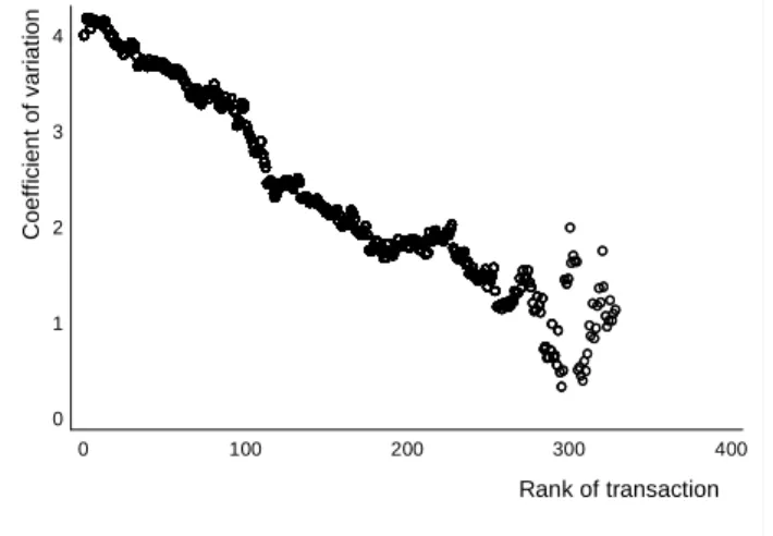
More interestingly, a new figure is proposed below to look at the dispersion of prices (coefficient of variation CV, i.e. standard deviation of prices per kilo divided by their mean) according to the rank of transaction. To the best of our knowledge, this is the first time that such a relationship is considered on fish auction markets. Combined with Fig. 3a, it shows that prices do not only decrease in levels within a day, but would also decrease in volatility (Fig.4). The decreasing pattern between price and transaction rank is convergent with the transaction up to a certain number of transactions (σ-convergence5). The disparity is reduced during the sales up to a certain number of transactions. The Ashenfelter hypothesis could then
5
The concept of σ-convergence is defined by the measurement of an indicator of disparity (e.g. CV) between different units and its development over time. Thus a convergence trend is present when the CV decreases, indicating a shrinking disparity of the variable.
be put forward, fitting with financial theory, where prices decline at higher ranks because the associated risk is lower, just like any other asset return.
0 1 2 3 4 C o e ff ic ie n t o f v a ri a ti o n 0 100 200 300 400 Rank of transaction
Fig. 4 Price per kg coefficient of variation and transaction rank
Source: University of Nantes, from RIC Data
4.3.2. Within a week
In Fig 5, a clear pattern of auction prices throughout the week is evidenced by the results, with higher price levels observed for the last days of the week (Friday and Saturday). Furthermore, whatever the day, the price appears to be decreasing with the transaction’s rank, but not immediately for the weekend days. We ran naive regression models for which the price is estimated according to the transaction’s rank for each day: prices during Tuesday and Wednesday appear to be more sensitive to the rank order on average, whereas Saturday or Monday’s prices appear to exhibit a less decreasing pattern.
Monday Tuesday Wednesday Thursday Friday Saturday 6 8 10 12 14 P re d ic te d p ri c e 0 100 200 300 400 Rank of transaction
Fig.5 Predicted price of transaction rank by type of
days
Note: Symmetric nearest neighbour linear smoothers Source: University of Nantes, from RIC Data
The different categories of buyers do not buy uniformly over the week days: mongers buy relatively more on the weekend, representing a 61% market share on Saturday (against 54% on average), while supermarkets and wholesalers are more present at the beginning of the week (Table 3). This could result in a specific price pattern on Saturday sales because of this composition effect between different bidder groups. The larger presence of mongers on Friday and Saturday goes with higher average prices and a greater number of lots (ranks).
Table 3
Daily statistics and market shares by types of day
(N = 66,834 transactions between September 1st, 2010 and September 29th, 2012)
Average Prices (euros) Average Quantities (tons) Average Rank (number) Market shares (%) Supermarkets Primary processors Fishmongers Monday – 9.30 – 110.93 – 105.90 + 13.42 + 32.37 – 51.22 Tuesday – 9.19 – 159.82 – 97.85 + 15.39 + 31.59 – 50.69 Wednesday – 8.82 + 238.47 + 127.16 – 11.90 – 28.18 + 56.86 Thursday – 8.80 + 207.04 – 115.54 + 13.89 + 36.84 – 46.71 Friday + 10.49 + 245.30 + 124.26 – 11.46 + 32.51 + 54.58 Saturday + 11.01 + 226.36 + 166.61 – 7.55 – 27.50 + 61.02 Average 9.67 99.07 122.18 11.99 31.33 53.97
Note: Among type of buyers, Others’ category omitted. +/‒ signifies that the value is higher/lower than its mean.
Source: University of Nantes, from RIC data
4.3.3. Within a year
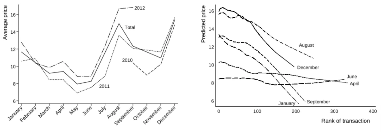
Some authors have linked the declining price anomaly to the irregularity of supply in the case of wild-caught fish markets (Christou 2000, Neugebauer and Pezanis-Christou 2007). Supply uncertainty would affect buyers’ preferences and perception about the available quantity on the markets, thus creating conditions for asymmetry and distinct risk behaviours. In the case of Nephrops markets, the best conditions for supply and demand do not fit: the high season for catches take place between April and June, meanwhile the peaks of demand concern August (because of coastal summer tourism) and December (Christmas demand). 2010 Total 2011 2012 6 8 10 12 14 16 A v e ra g e p ri c e Janu ary Febr uary Mar ch Apr il May June July Aug ust Sep tem ber Oct ober Nov em ber Dec em ber August December June April January September 6 8 10 12 14 16 P re d ic te d p ri c e 0 100 200 300 400 Rank of transaction
Fig. 6a Monthly average price Fig. 6b Predicted price and rank of transaction by
month
Note: Symmetric nearest neighbour linear smoothers.
Source: University of Nantes, RIC data
The monthly average prices were plotted in Fig. 6a, reflecting the two demand peaks of August and December, months of shortage. Prices have increased from year to year but present exactly the same seasonal patterns whatever the year. June represents a peak of tonnage for mongers (> 80 t), while May is more busy for the two other categories, but the market share of mongers is the highest for the summer months (July, August), close to 60%,
against 54% on average, certainly to meet the touristic demand. We ran naive regression models for which the price is estimated with respect to the transaction’s rank for each month. The declining price pattern is found more sensitive to the rank for the shortage months (January, December, September, October, August) and less sensitive for months with excess supply (March, April, June, and May).
5. The daily dynamics of prices with three buyer groups
Our first empirical strategy tests for the existence of a declining price within a day through the sequence of transactions by capturing the combined effects of several explanatory variables. Secondly, we search if actors behave similarly and how the presence of asymmetric buyer groups contributes to explain the daily price decrease.
5.1 The panel models
From the descriptive analysis of the data, we postulate that the price per kilo of traded lots can be explained by several factors. At the transaction level, we introduce in the model the effect of the lot size in order to capture its effect on prices, as shown in section 4.2. The price of the transaction is supposed to be explained by the rank of the transaction during the day. To scrutinize the daily dynamics, the 66,834 transactions have been divided into ten equally sized classes according to the rank order, each class representing a decile of the transactions’ distribution (up to the 12th transaction; then 12th to the 23rd; 24th to the 35th; 36th to the 49th; 50th to the 63rd; 64th to the 78th; 79th to the 95th; 96th to the 118th; 119th to the 155th, 156th and more.
Accounting for unobserved heterogeneity (to take into account the price variation across days), we consider an unbalanced panel in which each auction day i is characterized by a certain number of ranked transactions t. We obtain 547 days for which the average number of transactions is 122.2 (SD = 59.4; Min = 20; Max = 335; Q1 = 82; Q2 = 112; Q3 = 154) which corresponds to 66,834 transactions. We have a panel dataset in which both the rank of daily transactions and the number of days are quite large. However, due to the important variability in the daily number of transactions (from moderate to large), the panel is strongly unbalanced.
We choose first to estimate an Ordinary Least Square (OLS) model. To capture the day-invariant heterogeneity across groups, a Fixed-Effect (FE) model is estimated in a second step. By demeaning the variables using a within transformation, the fixed-effect estimator removes the effect of day-invariant observable characteristics so as the net effect of the explanatory variables on prices can be assessed. This estimator is designed in our case to study the causes of price variation within a day. However, in the FE models, only the intercept can differ across days. As the data are characterized by moderate to long T, we choose to estimate a model that allows for heterogeneous slope coefficients across days. The Mean-Group (MG) estimator (Pesaran and Smith, 1995) relies on estimating N daily regressions and averaging the coefficients. Furthermore, we suppose that the daily market may be characterized by a certain dynamic where learning and memories play an important role in this type of market (Vignes et al., 2011). The repeated transactions may be influenced by the daily dynamic and the lagged values of the price during the day. As the standard Least Square with Dummies Variables (LSDV) estimator of a dynamic panel provides biased and inconsistent estimates for finite time horizon (Nickell, 1981), we choose to estimate the bias
corrected least square dummy variables (LSDVC) estimator (Kiviet, 1995, 1999). The dynamic form of our model can be written as:
it i it it it P W u P =
γ
−1 +β
+ +ε
(1)where Pit is the vector of price (in logarithms) that vary between days i and transaction’s rank
t, Wit is a vector of variables described above, γ and βs are the corresponding parameters to
estimate, ui is the day-specific effect and εit is a residual error term expected to be
uncorrelated with the explanatory variables. In the OLS, FE, and MG models, we suppose that
γ is equal to 0. In the MG estimator, the equation (1) is estimated for each day including an
intercept to capture fixed effects (Eberhardt, 2012). The estimated coefficients are averaged across days:
∑
= = N i i N 1 ˆ 1β
β
(2)Finally, in the dynamic specification, a number of consistent instrumental variables (IV) and generalized method of moments (GMM) estimators have been proposed as an alternative to LSDV to remove the correlation between the transformed lagged dependent variable and the transformed error term (Anderson and Hsiao, 1982; Arellano and Bond, 1991; Blundell and Bond, 1998). With another approach, Kiviet (1995, 1999) chooses to compute an explicit data-dependent correction for the fixed-effects bias where the LSDVC removes an approximate sample bias from the FE estimator. The variance-covariance matrix of estimated coefficients is estimated by a bootstrap approach. Finally, Bruno (2005) computes the bias correction for unbalanced panels. According to Judson and Owen (1999) and Flannery and Hankins (2013), LSDVC dominates the GMM estimators for panel of all lengths for respectively balanced and unbalanced panels.
Table 4
Estimation results
OLS FE MG LSDVC
Lag of the price 0.8322***
(0.0060)
Lot size -0.1620*** -0.0206*** -0.0219*** -0.0069***
(0.0106) (0.00241) (0.0025) (0.0004)
Transaction ranks (deciles)
Less than 12 Ref. Ref. Ref. Ref.
12 lo less than 24 0.0139*** 0.0029 0.0023 -0.0022 (0.0032) (0.0030) (0.0030) (0.0012) 24 lo less than 36 0.0059 0.0002 0.0014 -0.0016 (0.0044) (0.0035) (0.0036) (0.0013) 36 lo less than 50 -0.0022 -0.0003 -0.0013 -0.0018 (0.0058) (0.0038) (0.0036) (0.0014) 50 lo less than 64 -0.0120* -0.0015 -0.0006 -0.0023* (0.0068) (0.0043) (0.0038) (0.0012) 64 lo less than 79 -0.0328*** -0.0087* -0.0070* -0.0034** (0.0077) (0.0047) (0.0040) (0.0013)
79 lo less than 96 -0.0547*** -0.0093* -0.0084** -0.0030** (0.0087) (0.0049) (0.0039) (0.0011) 96 lo less than 119 -0.1090*** -0.0144** -0.0083** -0.0043*** (0.0104) (0.0055) (0.0036) (0.0009) 119 lo less than 156 -0.1750*** -0.0236*** -0.0112*** -0.0064*** (0.0138) (0.0067) (0.0032) (0.0014) More than 156 -0.2390*** -0.0393*** -0.0090*** -0.0088*** (0.0208) (0.0119) (0.0028) (0.0012) Constant 2.804*** 2.358*** 2.435*** (0.0331) (0.0070) (0.0152) Number of days 547 547 547 547
Average number of rank 122.2 122.2 122.2 121.2
Number of observations 66834 66834 66834 66287
Note: Standard errors are in parenthesis. * p<0.1, ** p<.05, *** p<0.01. The type of buyer is taken into account (fishmonger, primary processor, supermarket, and other) but not presented here to focus on the rank effect.
Source: University of Nantes, RIC data
The estimates are presented in Table 4. The first model correspond simply the OLS estimates of the model (R2 = 0.19). In the FE model with White and clustered at the panel level standard errors6, the joint test of coefficient equality for the daily dummies rejects the null that the coefficients are equal to zero (F(546, 66274) = 1363.3, p = 0.000). However, the intra-day correlation is very high: nearly 95% of the variance is due to differences across days (R2 Within = 0.05, R2 Between = 0.48, R2 = 0.16). This reflects the strong variability of prices from day to day (e.g. weekday and seasonal effects). With a Hausman test, the hypothesis that the daily-level effects can be adequately modeled by a random effect model is rejected (Chi2(13) = 921.6, p = 0.000). The individual effects are correlated with the other regressors in the model.7 Furthermore, the MG estimator allows for slope coefficients heterogeneity across days. Pesaran and Smith (1995) show that the MG estimator will produce consistent estimates of the average of the parameters. This estimator does not consider nonetheless that certain parameters might be similar across groups to the traditional pooled estimators, such as the FE estimators. Finally, the LSDVC estimator takes into account the daily dynamics. Due to the important number of observations, the computationally simpler Anderson and Hsiao estimator is the chosen initialization and a parametric bootstrapped procedure with 50 replications is used to estimate the variance-covariance matrix.
5.2 A verified -although late- decline of price
In the four specifications, a negative relationship is found between the lot size and its price per kg8. The buyers who buy larger lots benefit on average from reduced price per kg.
6
As the Wooldridge to test for autocorrelation rejects the absence of first-order correlation (F(1,546) = 1001.9, p = 0.000), the standard errors are daily clustered. The modified Wald test for groupwise heteroskedasticity is strongly rejected (Chi2(547) = 81712.4, p = 0.000): White standard errors are used. The OLS specification has White and clustered at the panel level standard errors.
7
As the Frees (1995) and Pesaran (2004) tests of cross sectional independence are rejected, a FE model with Driscoll-Kraay standard errors was estimated with 4 lags. Even if the standard errors were increased due to contemporaneous correlation correction, the significance levels were not modified.
8
In order to check for potential endogeneity of lot size variable, instrumental variable estimator was tested with the FE model. The Hansen test of over-identifying restrictions cannot be rejected (Chi(1) = 0.994, p = 0.319) whereas the underidentification test is rejected (Chi(2) = 39.47, p = 0.000), when the lot size is instrumented by its second and third lagged difference values. In this case, the equivalent Durbin-Hu-Hausman test of endogeneity cannot reject that the variable can be treated as exogeneous (Chi(1) = 1.491, p = 0.222).
This could stem from different factors. Bigger lots are more likely to be purchased by primary processors or supermarket buyers for their secondary markets, than by mongers selling directly to consumers after the auction process. The negative parameter of the weight variable might therefore be interpreted in terms of lower competition in the bidding process for larger lots, or to a price discrimination effect where traders expect to pay a discounted unit price when buying a larger quantity.
In order to capture the daily dynamics of prices, the rank of transaction was firstly tested as a continuous variable and its quadratic form tested. Whatever the specification, the transaction rank is conversely linked to the log of the transaction price, without quadratic form. In approximately 75% of the 547 daily regressions used to construct the MG estimator, the rank of transaction is negative and significant at 5% level (431 days). The rank variable was then divided into ten ordered categories of transactions, each representing a decile of the distribution. We can see that after the 65th lot, the daily price decreases significantly in all tested models (similar results are obtained if other categories are taken as a reference). The latest daily transactions are associated with lower prices. Other FE models were run with deciles calculated day by day whatever the number of transactions (e.g. a first category representing less than 10% of the daily lots, a second one including the 10 to 20% first transactions, etc.). Another evidence of the declining pattern is obtained after that 60% of daily lots have been sold on average.
Increasing coefficients by rank category means that the declining pattern tends to be more acute at the end of the process, especially for long selling days (i.e. those including more than 156 transactions)9. For instance, in the fixed model, if a Wald test of coefficient equality between the two last categories (119 to less than 156 and 156 and more) shows that coefficients are not significantly different (F(1, 546) = 1.87, p = 0.173), we found significant differences for all other categories beyond the 65th lots taking the last category as reference.
In the LSDVC, even if the lagged price capturing the dynamics is significant and explain more than 80% of the price change in the short run (i.e. for the following transaction), the daily price starts to decrease significantly (at the 10% level) after the 50th lot. Interestingly, although the dynamic model is driven by the influence of past prices revealing a certain inertia of bidding behaviors (and possibly affiliation), the evidence of decreasing prices still remains.
5.3 Testing for asymmetric buying patterns
We have so far assumed that each category of buyers behaves similarly. To disentangle the buyer group effect and buyers’ behavior, we first present an OLS estimate including the weekday, month, and year effects in Table 5 (R2 = 0.61). The introduction of time effects confirms the estimates issued from Table 4: the late decline of prices. Furthermore, a clear pattern of auction prices throughout the week is evidenced by the results, higher price levels being observed for the last days of the week. A seasonal effect is also emphasized with the highest prices reached during the shortage months of August and December. Finally, the transactions purchased by primary processors and supermarkets are
9
As the panel is strongly unbalanced, the last averaged coefficients of the transaction rank variable in the MG model rely on fewer observations and should be taken with caution.
characterized by a lower price than fishmongers. Being the most largely represented category, fishmongers served as reference. We used a Wald test to see whether the coefficients between supermarkets and primary processors are equal. In this specification, the equality of coefficient is rejected at the 1% level [F(1, 546) = 56.00, p = 0.000]. From this result, it is clear that the average price paid by supermarkets is lower than the price paid by primary processors.
Table 5
Results by type of buyers
Symmetric buyers Asymmetric buyers
All buyers Fishmongers Primary Processors Supermarkets
Coeff SE Coeff SE Coeff SE Coeff SE
Lot size -0.088*** (0.007) -0.084*** (0.006) -0.082*** (0.009) -0.123*** (0.010)
Transaction ranks
Less than 12 Ref. Ref. Ref. Ref.
12 lo less than 24 0.008*** (0.003) 0.006 (0.005) 0.010 (0.007) 0.016** (0.007) 24 lo less than 36 0.001 (0.004) 0.004 (0.006) -0.004 (0.007) 0.001 (0.008) 36 lo less than 50 -0.006 (0.005) -0.006 (0.006) -0.011 (0.008) 0.001 (0.009) 50 lo less than 64 -0.013** (0.006) -0.008 (0.007) -0.021** (0.009) -0.015 (0.009) 64 lo less than 79 -0.032*** (0.007) -0.035*** (0.008) -0.034*** (0.010) -0.014 (0.010) 79 lo less than 96 -0.044*** (0.007) -0.041*** (0.008) -0.050*** (0.010) -0.039*** (0.011) 96 lo less than 119 -0.068*** (0.008) -0.072*** (0.009) -0.060*** (0.011) -0.065*** (0.012) 119 lo less than 156 -0.097*** (0.010) -0.101*** (0.011) -0.088*** (0.012) -0.094*** (0.012) More than 156 -0.142*** (0.015) -0.151*** (0.016) -0.126*** (0.017) -0.144*** (0.019) Weekday
Monday Ref. Ref. Ref. Ref.
Tuesday 0.036 (0.034) 0.018 (0.034) 0.055 (0.035) 0.075** (0.030) Wednesday -0.013 (0.032) -0.027 (0.033) -0.003 (0.033) 0.020 (0.030) Thursday -0.025 (0.032) -0.039 (0.039) -0.013 (0.034) 0.019 (0.029) Friday 0.149*** (0.033) 0.129*** (0.034) 0.169*** (0.035) 0.188*** (0.031) Saturday 0.185*** (0.037) 0.168*** (0.037) 0.204*** (0.039) 0.211*** (0.034) Month
January Ref. Ref. Ref. Ref.
February -0.052 (0.047) -0.052 (0.048) -0.050 (0.048) -0.076* (0.044) March -0.165*** (0.034) -0.168*** (0.035) -0.160*** (0.035) -0.153*** (0.032) April -0.142*** (0.039) -0.138*** (0.040) -0.142*** (0.041) -0.127*** (0.037) May -0.295*** (0.035) -0.290*** (0.038) -0.294*** (0.036) -0.277*** (0.033) June -0.270*** (0.034) -0.267*** (0.036) -0.269*** (0.035) -0.263*** (0.032) July -0.064* (0.036) -0.066* (0.036) -0.057 (0.037) -0.058 (0.037) August 0.277*** (0.036) 0.266*** (0.037) 0.301*** (0.037) 0.283*** (0.033) September 0.168*** (0.038) 0.163*** (0.038) 0.185*** (0.040) 0.135*** (0.037) October 0.047 (0.047) 0.050 (0.048) 0.059 (0.050) 0.001 (0.044) November 0.108** (0.045) 0.110** (0.045) 0.115** (0.047) 0.085** (0.043) December 0.384*** (0.059) 0.386*** (0.057) 0.394*** (0.066) 0.333*** (0.060) Year
2010 Ref. Ref. Ref. Ref.
2011 0.117*** (0.034) 0.117*** (0.034) 0.120*** (0.037) 0.099*** (0.034) 2012 0.275*** (0.037) 0.277*** (0.037) 0.280*** (0.039) 0.226*** (0.036) Buyer group Fishmongers Ref. Supermarkets -0.030*** (0.003) Primary processors -0.007*** (0.003)
Constant 2.400*** (0.049) 2.426*** (0.050) 2.390*** (0.055) 2.491*** (0.051)
Number of obs. 66834 66834
Note: White standard errors (in parenthesis) clustered by date. Among type of buyers, Others’ category omitted. * p<0.1, ** p<.05, *** p<0.01.
Source: University of Nantes, RIC data
Now assuming that the declining price pattern is affected by the presence of asymmetric buyers, we specify an asymmetric model by using the interaction of each variable issued from the symmetric one with each type of buyers (which gives the coefficients that would be obtained if separate models were estimated for each type of buyers). Buyers behave on average differently with regard to the lot size: the Wald test of coefficient equality is strongly rejected [F(2, 546) = 26.00, p = 0.000]. The lot size has greater influence on prices for supermarkets than for any other buyer group. In the same way, the decline of prices over the sales is slower for supermarkets than for any other category. It starts, on average, after the 79th lot, against the 64th lot for mongers and the 50th lot for primary processors. A joint Wald test of transactions’ rank coefficients shows that trend patterns on prices differ between actors [F(18,546) = 2.13, p = 0.004]. However, the effect of this dynamic on prices does not differ between fishmongers and supermarkets [F(9,546) = 1.32, p = 0.226] and between primary processors and supermarkets [F(9,546) = 1.45, p = 0.164]. But a significant difference is found between fishmonger and primary processors [F(9,546) = 2.61, p = 0.006]. Interestingly, the coefficient if the category ‘12 to less than 24’ is significant for supermarket (compared to the ‘Less than 12’ one) which means that supermarkets are in average prone to pay higher prices at the beginning of the transaction’s day. Then, the declining price phenomenon concerns all buyer categories, even if differences of coefficients can be found across categories in periods of higher demand (weekday, high season). A joint Wald test of weekdays coefficients shows that the effect of weekday patterns on prices differ between actors [F(10,546) = 3.41, p = 0.000], although no significant difference was found between supermarkets and primary processors [F(5,546) = 1.64, p = 0.147]. Similarly, a joint Wald test of monthly coefficients shows that the effect of monthly patterns on prices differ between actors [F(20,546) = 2.77, p = 0.000] and for each pair of actors.
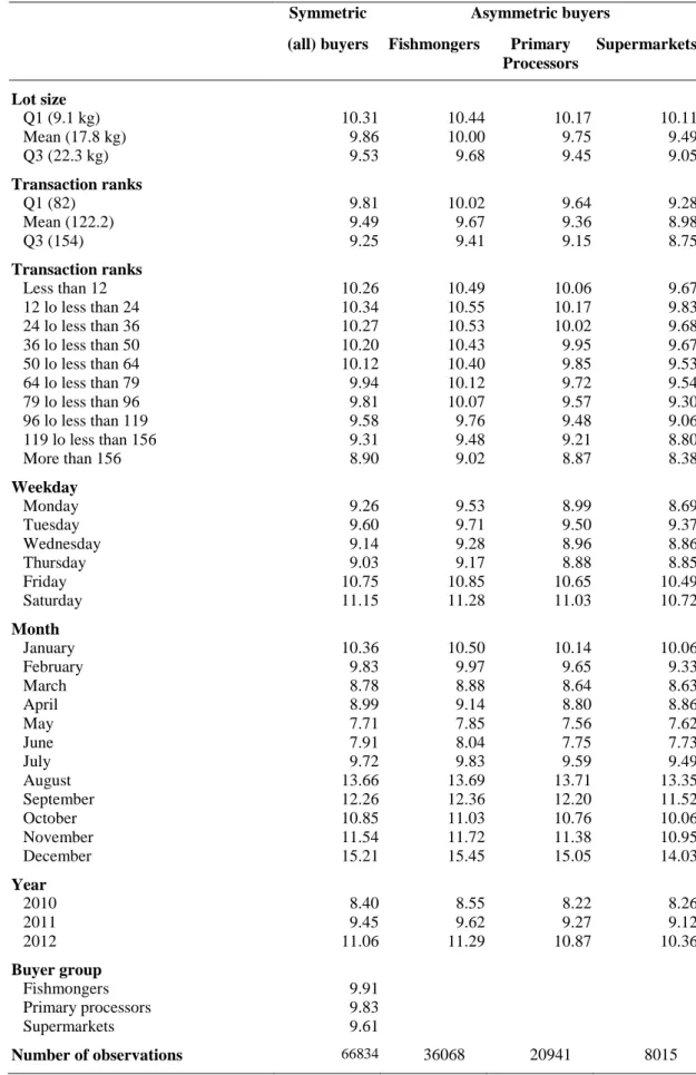
In Table 6, the average predicted prices have been calculated. The Table exhibits strong differences according to the lot size, transaction ranks, weekdays, months, and years. We can outline the closeness of average predicted prices between supermarkets and primary processors for small lots, the difference increasing with the size of lots. As far as weekdays are concerned, when prices are lower (from Tuesday to Thursday), price differences between buyer groups are less significant than Saturday, when fishmongers “make” the market price (the gap between supermarket and mongers’ price then representing 0.56 €/kg). Similarly, price differences are less significant between groups during the months of excess supply, between March and July, reaching 1.42 €/kg between mongers and supermarket buyers. Of greater interest for our study is the price difference between the beginning and the end of sales (rank effect): all buyers included, the price decreases by 1.36 €/kg, which makes a huge drop in revenues for fishers. This gap takes even greater values for fishmongers (-1.47 €/kg), than for the two other categories (-1.29 €/kg for supermarkets and -1.19 €/kg for primary processors).
Table 6 Average predicted price (Euros/kg)
Symmetric Asymmetric buyers
(all) buyers Fishmongers Primary
Processors Supermarkets Lot size Q1 (9.1 kg) 10.31 10.44 10.17 10.11 Mean (17.8 kg) 9.86 10.00 9.75 9.49 Q3 (22.3 kg) 9.53 9.68 9.45 9.05 Transaction ranks Q1 (82) 9.81 10.02 9.64 9.28 Mean (122.2) 9.49 9.67 9.36 8.98 Q3 (154) 9.25 9.41 9.15 8.75 Transaction ranks Less than 12 10.26 10.49 10.06 9.67 12 lo less than 24 10.34 10.55 10.17 9.83 24 lo less than 36 10.27 10.53 10.02 9.68 36 lo less than 50 10.20 10.43 9.95 9.67 50 lo less than 64 10.12 10.40 9.85 9.53 64 lo less than 79 9.94 10.12 9.72 9.54 79 lo less than 96 9.81 10.07 9.57 9.30 96 lo less than 119 9.58 9.76 9.48 9.06 119 lo less than 156 9.31 9.48 9.21 8.80 More than 156 8.90 9.02 8.87 8.38 Weekday Monday 9.26 9.53 8.99 8.69 Tuesday 9.60 9.71 9.50 9.37 Wednesday 9.14 9.28 8.96 8.86 Thursday 9.03 9.17 8.88 8.85 Friday 10.75 10.85 10.65 10.49 Saturday 11.15 11.28 11.03 10.72 Month January 10.36 10.50 10.14 10.06 February 9.83 9.97 9.65 9.33 March 8.78 8.88 8.64 8.63 April 8.99 9.14 8.80 8.86 May 7.71 7.85 7.56 7.62 June 7.91 8.04 7.75 7.73 July 9.72 9.83 9.59 9.49 August 13.66 13.69 13.71 13.35 September 12.26 12.36 12.20 11.52 October 10.85 11.03 10.76 10.06 November 11.54 11.72 11.38 10.95 December 15.21 15.45 15.05 14.03 Year 2010 8.40 8.55 8.22 8.26 2011 9.45 9.62 9.27 9.12 2012 11.06 11.29 10.87 10.36 Buyer group Fishmongers 9.91 Primary processors 9.83 Supermarkets 9.61 Number of observations 66834 36068 20941 8015
Note: Exponentiated average predicted prices. Others’ category omitted.
6. Discussion
The objective of the present research was to highlight the anomaly of decreasing prices within daily auction sales and to explain such a paradox through asymmetric behaviours of bidders. The Vickrey theorem of revenue equivalence between identical auctioned items sold sequentially (Vickrey 1961) would not hold throughout time because at least one of the axiomatic conditions –namely non-affiliation, risk-neutrality and symmetry of bidders- is not met. Our results confirm the presence of such declining price anomalies on a French market for Nephrops with sequential Dutch auctions. Auction prices tend to decrease significantly after a certain number of transactions, i.e. after rank 65 on average (122 being the average number of daily transactions). A similar negative relationship was also observed in other European fish markets operating under a descending auction process, such as the Spanish market of Palamós for fish (Fluvià et al. 2012) and the Ancona market in Italy (Gallegatti et al. 2011). On the Spanish market, a price decline was only found for 8 of the 12 species, but not for small Nephrops. A different trading system (through pairwise transactions) may lead to different outcomes, since the case of the Marseilles fish market showed no such phenomenon (Härdle and Kirman 1995).
Several hypotheses can explain the declining price anomaly. First of all, the symmetry condition does not hold, thus considering different buyer groups under the market with distinct private values and possibly various risk attitudes. This can be the case of small vs large buyers, the latter bidding more aggressively to obtain the required quantity meanwhile the former group can afford to wait for better conditions due to smaller procurements. Buyers may also occupy different positions within the market chain, being more or less close to consumers and therefore able to extend their margins more easily. They may also value time differently, being more impatient to leave the market as they need to open their distant retail shop. A second hypothesis may lie in the changing market structure throughout the sequence of transactions. A diminishing number of bidders would result in oligopsonistic and more collusive behaviours in the course of time, reducing the price levels for the latest transactions. Finally, a third hypothesis which is not independent from the two previous ones associates the declining price anomaly with supply uncertainty and periods of shortage. When the market is short in tonnage and buyers face demand peaks, then risk-averse bidders would tend to bid more aggressively during the first transactions and, once served, would leave the market earlier.
In the present case, stylized facts (section 4) and model estimations (section 5) shed new light to the price decline anomaly. Periods of higher supply clearly smooth down the anomaly, as shown by Pezanis-Christou (2000) for sardine lots auctioned in May in Sète. Uncertainty about the total number of units produces the paradox, which disappears otherwise. The available quantity of the day with regard to the demand level matters for bidders, both by signaling excess supply to the whole market and by producing a lower fear of bidders for not being served during early transactions. This variable was also found very significant and negative for all the 12 models tested in Fluvià et al. (2012) and by Gallegatti et
al. (2011). In the latter article, authors have also noticed, after ranking the transactions, that
the average price goes down as the rank increases. They calculated the price variation for the last two transactions of the day, and showed that “the average price tends to increase on days
characterized by a limited supply of fish” (Ibid., p. 27). The limited supply plays a key role
not only during the early sales (risk premium included in the price, as reported by McAfee and Vincent 1993) but also at the very end of the sales, when some buyers realize that they do not have the quantity demanded by their own customers.
The perception about shortage and excess supply might be different for buyer groups. Here comes another argument served by Pezanis-Christou (2000). Wholesalers are distinguished from retailers who buy fewer and smaller lots at higher prices, and may leave the market earlier, as reported also in Gallegatti et al. (2011). In our present study, a third buyer category (supermarket buyers) seems to behave differently from both primary processors and mongers. They purchase at lower prices, exhibit greater (negative) influence of the lot size on prices, and auction prices decrease more lately for them (rank 79), than for the two other groups (rank 64 for fishmongers, and rank 50 for processors). This latter variable must be understood as a proxy of bidding aggressiveness, showing longer –hence stronger- interest of supermarkets to buy fish lots.
This may appear as a second paradox since supermarket buyers bid more aggressively while paying lower prices. The reason lies in the market time picked up by supermarkets, i.e. weekdays and more abundant seasons, when they can advertise for campaign prices (large tonnage at low shelf prices) in their own multiple retail shops. On the other hand, weekend sales are preferably targeted by the other small retailers (mongers), resulting in a greater number of smaller lots on Saturday (167 ranks, versus 122 on average) and thus reduce the price decline anomaly that particular day. An evidence of this phenomenon is given by the predicted price differences between the beginning and the end of the sales by buyer group and by weekday or month. For example, price gaps are larger between supermarket and fishmongers on Saturday, when the latter buyers “make” the market price, than on a mid-week day. This is even more obvious when comparing the difference of predicted prices between buyer groups in June (-0.23 €/kg) and in December (-1.42 €/kg). Consequently, the fall in prices between the first and last range of transactions becomes logically smaller for supermarkets (-1.29 €/kg) than for fishmongers (-1.47 €/kg).
On the basis of a KS test, Pezanis-Christou (2000) also found that distinct categories of buyers had different preferences regarding the timing of transactions, one type of buyer buying significantly earlier than others. We have conducted a similar test with a normalized rank index variable (for each day, the rank associated to the transaction is divided by the daily total number of transactions). A test of equality of medians (nonparametric K-sample test on the equality of medians) of this index rejects the null hypothesis of the same median for all buyer groups. The supermarket distribution is characterised by a median value which differs from that of primary processors and fishmongers, whereas the null hypothesis is accepted for these two latter groups10. A Wilcoxon ranksum test (Mann-Whitney test) gave similar results. The estimation of the probability that a random draw from the mongers’ distribution is higher than a random draw from the processors’ one is not significantly different from 0.5, whereas probability that the transaction rank for fishmongers or primary processors is greater than the transaction rank for supermarkets is 0.58.
10 Between supermarkets and primary processors, Chi2(1) = 324.67, p. = 0.000; between supermarkets and
fishmongers, Chi2(1) = 405.34, p. = 0.000, and between primary processors and fishmongers, Chi2(1) = 2.04, p. = 0.153)