HAL Id: hal-00838867
https://hal-ensta-paris.archives-ouvertes.fr//hal-00838867
Submitted on 4 Jun 2015HAL is a multi-disciplinary open access archive for the deposit and dissemination of sci-entific research documents, whether they are pub-lished or not. The documents may come from teaching and research institutions in France or abroad, or from public or private research centers.
L’archive ouverte pluridisciplinaire HAL, est destinée au dépôt et à la diffusion de documents scientifiques de niveau recherche, publiés ou non, émanant des établissements d’enseignement et de recherche français ou étrangers, des laboratoires publics ou privés.
Transition scenario to turbulence in thin vibrating plates
Cyril Touzé, Stefan Bilbao, Olivier Cadot
To cite this version:
Cyril Touzé, Stefan Bilbao, Olivier Cadot. Transition scenario to turbulence in thin vibrating plates. Journal of Sound and Vibration, Elsevier, 2012, 331 (2), pp.412-433. �10.1016/j.jsv.2011.09.016�. �hal-00838867�
Transition scenario to turbulence in thin vibrating plates
C. Touz´ea,∗, S. Bilbaob, O. Cadota
aUnit´e de M´ecanique (UME), ENSTA-ParisTech, Chemin de la Huni`ere, 91761 Palaiseau Cedex, France bAcoustics and Fluid Dynamics Group/Music, University of Edinburgh, James Clerk Maxwell Building,
Edinburgh, United Kingdom
Abstract
A thin plate, excited by a harmonic external forcing of increasing amplitude, shows transitions from a periodic response to a chaotic state of wave turbulence. By analogy with the transi-tion to turbulence observed in fluid mechanics as the Reynolds number is increased, a generic transition scenario for thin vibrating plates, first experimentally observed, is here numerically studied. The von K´arm´an equations for thin plates, which include geometric non-linear ef-fects, are used to model large amplitude vibrations, and an energy-conserving finite difference scheme is employed for discretization. The transition scenario involves two bifurcations sepa-rating three distinct regimes. The first regime is the periodic, weakly non-linear response. The second is a quasiperiodic state where energy is exchanged between internally resonant modes. It is observed only when specific internal resonance relationships are fulfilled between the eigen-frequencies of the structure and the forcing frequency; otherwise a direct transition to the last turbulent state is observed. This third, or turbulent, regime is characterized by a broadband Fourier spectrum and a cascade of energy from large to small wavelengths. For perfect plates including cubic non-linearity, only third-order internal resonances are likely to exist. For imper-fect plates displaying quadratic nonlinearity, the energy exchanges and the quasiperiodic states are favored and thus are more easily obtained. Finally, the turbulent regime is characterized in the light of available theoretical results from wave turbulence theory.
Keywords: transition scenario, thin plate, wave turbulence, bifurcation
1. Introduction
Turbulence and wave turbulence. Turbulence has always been a key research area in fluid me-chanics and is still considered as a partly unsolved (and perhaps unsolvable) problem due to fundamental limitations of analytical tools in the case of an infinite hierarchy of cumulant equa-tions [1, 2]. Zacharov [3], however, introduced a so-called wave (or weak) turbulence (WT) theory which may be arrived at by relaxing some of the assumptions that are particularly rele-vant to fully developed hydrodynamics turbulence (in particular the presence of intermittency), but by retaining the main assumption of an energy flux through lengthscales allowing for the appearance of the Kolmogorov turbulence spectrum. The main assumptions of WT are that the nonlinearity is weak, and that waves persist in the dynamical behaviour of the system [4]. With this in mind, closed equations, the so-called kinetic equations, are analytically accessible,
∗Corresponding author
Email addresses: [email protected] (C. Touz´e), [email protected] (S.
and hence allow for quantitative predictions. Because of these tractable simplifications, the WT theory has been applied successfully to numerous physical systems including capillarity and gravity waves on the surface of liquids [5, 6, 7, 8], plasmas [9], optics [10] and magnetohydro-dynamics [11].
Turbulence in a solid. Wave turbulence theory can be applied to vibrating structures that can dis-play, when subjected to large-amplitude motions under a geometric non-linearity, a broadband Fourier component in the power spectrum of the displacement, revealing turbulent behaviour. In the musical context, the perceptual importance of this feature has been long since recognized in instrument design; for example, the broadband Fourier component has been exploited for a long time in theaters to simulate the sound of thunder by shaking vigorously large metallic plates. It is also the means of explaining the bright shimmering sound of gongs and cymbals [12, 13, 14, 15, 16]. From the physical point of view, this vibration state was first studied in the framework of chaotic behaviour for dynamical systems [17, 14, 18, 19]. However, convergence of traditional indicators of chaotic dynamics resulting from low-dimensional dynamical systems (e.g. correlation dimension and Lyapunov exponents) has been found from experiments only recently in a series of papers by Nagai et al. [20, 21, 22] where a shell of small dimensions was excited at moderate amplitudes, so that turbulent behaviour is not excited. Other experimental studies [23, 24, 13], as well as numerical results [25] reported difficulties in obtaining converged values for the correlation dimension and/or the Lyapunov exponents. Recently, wave turbulence theory has been applied to vibrating plates described by the von K´arm´an kinematical assump-tions, hence allowing for a quantitative prediction of the energy repartition through lengthscales [26], and two different experimental set-ups with very thin plates of large dimensions precisely accounted for turbulent behaviour [27, 28, 29]. More specifically, no intermittent behaviour was reported [27] and the persistence of waves has been clearly highlighted [29, 30], so that the main assumptions of WT are clearly verified experimentally.
Goal. The aim of this paper is to present numerical results allowing the study of the turbulent behaviour of plates, with or without imperfection, and this first part is more directly concerned with the transition to turbulence. First, experimental results indicate the generic transition sce-nario observed in thin structures like plates and shells, when they are excited pointwise with a harmonic forcing of increasing amplitude. This scenario has already been reported elsewhere for gongs and cymbals [12, 13, 14, 24, 31, 25]; here experimental results on a rectangular plate are presented, showing once again the generality of these observations. Next, a numerical model is presented, allowing for a precise reproduction of the experimental set-up. The model is based on a finite difference scheme that, in the lossless case, conserves energy to machine accuracy [32], and allows modelling of pointwise harmonic forcing. Preliminary numerical results have already been presented for a plate with free edges in [33]; here the case of simply-supported edges is considered. The transition scenario is then numerically assessed, for the case of perfect and imperfect plates. Finally, the turbulent state is briefly addressed by comparing the power spectrum of the numerically obtained velocity to that predicted in [26].
Summary of experimental results. The case of a thin structure (such as a plate, shell, gong or cymbal) excited pointwise with a harmonic forcing of a given frequency fexc and linearly increasing amplitude, is considered. Numerous observations have already been reported on var-ious kinds of gongs, cymbals and circular spherical-cap shells in [12, 13, 14, 34, 24, 31, 25], where the pointwise forcing is realized either with a mechanical shaker or with an electromag-netic device consisting of a magnet glued to the structure surrounded by a coil with controlled current, as described in [35, 36, 28]. The observed scenario for the transition to turbulence in
vibrating structures implies two bifurcations, separating three distinct regimes.
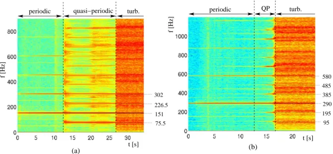
The case is here illustrated in Fig. 1, showing measurements drawn from a thin rectangular plate of lateral dimensions 38cm×29cm and thickness h=1 mm. The plate is excited at its centre by a shaker and has free edges. The vibration velocity is measured by a laser vibrometer, 2 centimeters from the center (to avoid laser saturation if measuring near the edges, as can occur in the turbulent regime where the vibration amplitude can be of the order of one centimeter). Fig. 1 shows two typical measurements obtained for excitation frequencies fexc=151 Hz and
290 Hz respectively. The excitation amplitude is increased linearly during the experiment, then maintained at a constant value once the turbulent regime is attained. Spectrograms of the measured velocity are shown, with time indicated on the abscissa.
f [Hz] (b) t [s] periodic QP turb. f [Hz] t [s] periodic quasi−periodic (a) turb. 75.5 151 226.5 302 95 195 290 385 485 580
Figure 1:Experimental spectrograms of the vibration velocity for a rectangular plate excited with a har-monic force of increasing amplitude and frequency 151 Hz (a), and 290 Hz (b). In each case the three different vibration regimes are clearly identified.
For small excitation amplitude, the regime is moderately nonlinear. In order to optimize the injection of energy, fexc is generally chosen in the vicinity of one of the structure’s linear eigenfrequencies. Hence the first regime is essentially a nonlinear unimodal regime, where the directly excited mode vibrates in the nonlinear regime, characterized by the appearance of harmonics of the forcing in the response. In the two cases, harmonics of order 2 to 4 are clearly visible; as imperfections are unavoidable in real plates [37], quadratic nonlinearity is present, and these even harmonics are observed in the response. Note the presence of harmonics of 50 Hz in the response, at small and constant levels. They are related to the current delivered and are unavoidable in measurements. They are easily recognizable and must not be interpreted as physical.
For a given excitation amplitude level, a bifurcation is observed. In Fig. 1(a), a 1:2 inter-nal resonance is excited, and energy is transferred from the directly excited mode to that with eigenfrequency near fexc/2. Modal analysis reveals the existence of an eigenmode at frequency
72 Hz, which is here slightly shifted by the nonlinearity and lock-in phenomena to perfectly fulfill the 1:2 resonance relationship and receive energy from the directly excited mode. The bifurcation is clearly delimited, as is usual in 1:2 internal resonance where a subcritical bi-furcation is at hand [38, 39, 40]. Consequently the jump to the coupled branch excites higher
frequencies resulting in a short transient. Then the coupled 1:2 regime sets in clearly, and finally appears to be disturbed in the vicinity of the second bifurcation. For fexc= 290 Hz, Fig 1(b),
the first regime becomes unstable in favour of a coupled regime involving two eigenmodes, whose eigenfrequencies f1 =95 Hz and f2 =195 Hz are such that f1+ f2 = fexc, resulting in a
1+1:2 internal resonance relationship. Once again, linear analysis reveals the presence of two eigenmodes at 90 and 190 Hz respectively, again with frequencies slightly shifted to fulfill the resonance condition. From these two examples and those already presented in [13, 14, 25], the generic scenario experimentally observed involves thus a first bifurcation where all the modes sharing internal resonance relationships of the form :
fi+ fj = fexc (1)
are excited through energy exchange, leading to a so-called quasiperiodic state. The simple case of 1:2 internal resonance is a particular case of (1) where fi = fjleading to a quasiperiodic
state degenerated in a periodic regime. The frequency peaks appearing in the quasiperiodic regime can also not be directly related to the excitation frequency. The energy can first be spread through modes sharing internal resonance with the directly excited modes like (1), then, once this new subset of frequencies is excited, new modes sharing a resonance relationship of the form fn± fp = fk with at least one of fn, fp or fk belonging to the first subset of excited
modes, can appear in the vibration. In all the experiments realized, order-two internal resonance relationships have always been observed, which simply reflect the fact that for real plates with imperfections, quadratic nonlinearities dominate those of cubic type, so that order-three internal resonance relationships are completely hidden by those of second order. Fig. 1 shows two excitation frequencies for which the quasiperiodic regime appears, but it may not be present if no evident internal resonance relationships exist. This has been observed preferentially for low-frequency excitations, as the coupling appears to be with modes with frequency smaller than that of the excitation.
Finally, the second bifurcation occurs and the turbulent regime sets in. It is characterized by a broadband Fourier spectrum with energy up to 8000 Hz for the two cases shown in Fig 1, indicating a flux of energy from the injection scale to the dissipative scale.
The aim of this paper is to develop an efficient numerical method in order to study the transition to turbulence through simulations, allowing validation of the scenario inferred from experimental measurements, as well as to give more insight to turbulent behaviour.
2. Numerical model
2.1. The von K´arm´an equations for perfect and imperfect plates
The model chosen here relies on the von K´arm´an kinematical assumptions for describing the geometric (large-amplitude) non-linear behaviour of thin plates. A rectangular plate of dimensions Lx× Lyand thickness h is considered, and is of elastic material of density ρ, Young’s
modulus E and Poisson’s ratio ν. The equations of motion are given for an imperfect plate without residual stresses, and comprise a set of two equations for the two unknowns, namely the transverse displacement ¯w(x, y, t) and the Airy (or stress) function ¯F(x, y, t) [41, 42, 43, 37]:
ρh ¨¯w + D∆∆ ¯w + ¯σ0w = L( ¯˙¯ w, ¯F) + L( ¯w0, ¯F) + ¯p, (2a) ∆∆ ¯F = −Eh
where D = Eh3/12(1 − ν2) is the flexural rigidity, ¯σ
0 is an ad hoc viscous damping coefficient,
and ¯p represents the external forcing applied to the plate. The geometric imperfection is repre-sented by the displacement ¯w0(x, y, t) of the middle surface. In setting ¯w0 = 0, the von K´arm´an
equations for perfect plates are recovered. The bilinear operator L is defined, in Cartesian coor-dinates, as:
L(F, w) = F,xxw,yy+ F,yyw,xx− 2F,xyw,xy (3)
The equations (2) are scaled by using the following transformations:
x = ¯x pLxLy , y = ¯y pLxLy , w = p 6(1 − ν2) h w¯ (4a) F = F¯ D, σ0 = ¯ σ0 ρh, p = p 6(1 − ν2) ρh2 ¯p (4b)
After substitution, we obtain: ¨
w + κ2∆∆w + σ0w = κ˙ 2L(w + w0, F) + p, (5a)
∆∆F = −L(w, w + 2w0), (5b)
where κ2 = D
ρhL2
xL2y. The equations of motion (5) will be used in the remainder of the article. It is worth noting that they are not non-dimensional equations: time has not been scaled, so that the factor κ has the dimension of a frequency. This choice has been retained for computational reasons.
In the remainder of the paper, simply supported boundary conditions are chosen. For the scaled transverse displacement w, simplified boundary conditions are used [44, 45, 16]:
w = 0, ∂ 2w ∂x2 = 0; for x = 0, s Lx Ly ; ∀y (6a) w = 0, ∂ 2w ∂y2 = 0; for y = 0, s Ly Lx ; ∀x. (6b)
For the scaled Airy stress function F the following boundary conditions have been cho-sen [45]: F = 0, ∂F ∂x = 0; for x = 0, s Lx Ly ; ∀y (7a) F = 0, ∂F ∂y = 0; for y = 0, s Lx Ly ; ∀x (7b)
2.2. Finite difference scheme
In this section a finite difference scheme is introduced to solve the equations of motion (5) together with boundary conditions (6)-(7). The scheme is a perfectly energy-conserving scheme (under lossless conditions), to machine accuracy, and has been introduced in [32]. It is here adapted to the case of forced and damped equations.
2.2.1. Grid functions and operators
The main steps for deriving the energy-conserving scheme are here briefly recalled, fol-lowing the notations and the definitions given in [16, 32]. For more thorough details on the discrete operators, the reader is referred to [16], and to [32] for the proof that the scheme is energy-conserving for undamped and unforced equations.
The continuous unknown functions w(x, y, t) and F(x, y, t) are replaced by their values on a discrete domain: wnl,m and Fl,mn , for integer l, m and n. The time index is n where continuous time t has been replaced by its discrete counterpart tn = nht with ht the time step. In the
same manner, the spatial domain is discretized so that the indices l, m are defined through: (l, m) ∈ [0, Nx] × [0, Ny]. The size of the domain is (Nx + 1)(Ny + 1), and the space steps are
denoted respectively by hx and hy. In practice, the grid spacings hx and hy are fixed by the
stability condition of the scheme (see below), and the number of grid points is deduced from Nx = E(h1x q Lx Ly) and Ny = E( 1 hy q Ly
Lx), where E(⊺) stands for the integer part of ⊺. For minimal numerical dispersion effects, it is best to choose the grid spacings as close to these bounds as possible, for a given time step.
The following discrete notations are now introduced. The unit forward and backward time shift operator are defined through their action on a grid function, say wnl,m, as:
et+wnl,m= wn+1l,m , et−wnl,m = wn−1l,m. (8)
Classical approximations of the first (centered, forward and backward) and second derivatives in time read as:
δt. = 1 2ht (et+− et−), δt+ = 1 ht (et+ − 1), δt− = 1 ht (1 − et−), δtt =δt+δt−, (9)
where ”1” stands for the identity operator. Temporal averaging operator are defined as:
µt+ = 1 2(et+ + 1), µt− = 1 2(1 + et−), µt. = 1 2(et+ + et−), µtt= µt+µt−, (10) The same definitions clearly follow for the spatial discrete variables, where we will also need a discrete bi-Laplacian (or biharmonic) operator δ∆∆ defined from:
δ∆= δxx+δyy (11)
δ∆∆ = δ∆δ∆ (12)
2.2.2. Conservative scheme
The two-parameter family of energy-conserving schemes (or monotonically dissipative in the lossy case) introduced in [32] is here adapted to the case of the damped and forced problem defined by (5). For the sake of simplicity, the discrete variables wn
l,mand F n
l,mare simply denoted
by w and F. The family of schemes depends on two parameters named β and γ, as:
δttw = −κ2δ∆∆w − σ0δt.w + κ2l( ˜w + ˜w0, ˜F) + pn
l,m, (13a)
µt−δ∆∆F = −γl(w, et−(w + 2w0)) − (1 − γ)µt−l(w, w + 2w0). (13b)
where the following terms, directly depending on the two parameters β and γ, have been intro-duced: ˜ w = γw + (1 − γ)µt.w, (14a) ˜ w0 =γw0+ (1 − γ)µt.w0, (14b) ˜ F = βF + (1 − β)µt.F. (14c)
The bilinear operator L has been discretized as l(w, F) and reads:
l(w, F) = δxxw δyyF + δyyw δxxF − 2µx−µy−(δx+y+w δx+y+F). (15)
The external forcing is introduced so as to mimic the experimental results described in the introduction. Consequently, the dimensioned forcing has been chosen as
¯p( ¯x, ¯y, t) = δ( ¯x − ¯x0)δ(¯y − ¯y0) ¯A sin(Ωt), (16)
where ¯A is the amplitude of the forcing (in N), and Ω the excitation frequency. The non-dimensional forcing simply reads:
p(x, y, t) = δ(x − x0)δ(y − y0) A sin(Ωt), with A = p 6(1 − ν2) ρh2L xLy ¯ A (17)
The forcing is pointwise, so that the discretized forcing term pnl,m appearing in Eq. (13a) is bilinearly spread to the four nearest neighbours of the chosen excitation point (x0, y0).
The stability condition, which may be derived through energy analysis, is:
β ≤ 1/2 (18a) ht ≤ h2 xh2y 2(h2 x+ h2y) r ρh D (18b)
under the choice of γ = 1 and β = 0. It is worth emphasizing that this condition, identical to that which holds in the linear case, is here necessary and sufficient for stability in the fully nonlinear case as well.
In practice, the sampling rate fS is chosen a priori, and the number of grid points for the
simulation is chosen so as to satisfy the above condition as closely as possible, thus minimizing numerical dispersion effects.
3. Simulation results for the perfect plate 3.1. Linear convergence
For the simulations, a plate has been chosen with dimensions Lx = 0.4m × Ly = 0.6m, and
thickness h=1 mm. Material parameters have been set so as to model a steel plate, with E= 200 GPa, ν=0.3 and ρ=7860 kg.m−3.
For a simply-supported plate, the radian frequencies are known analytically [44]:
ωapq =π2 s D ρh " p2 L2 x + q 2 L2 y # , (19)
where p and q are two integers indicating the number of half-waves in the x and y directions respectively. Table 1 shows the first 27 exact eigenfrequencies of the chosen plate, ranging from 21.65 Hz (fundamental mode) to 406.29 Hz.
The linear problem associated with (5) allows estimation of the numerical eigenfrequen-cies computed with the finite-difference scheme. As usual with finite differences, a fine grid is necessary in order to have significant accuracy in the computed frequencies, and the accuracy
21.65 41.63 66.61 74.93 86.59 119.89 121.55 141.54 161.52
166.52 181.50 194.82 226.46 241.44 246.44 254.76 266.42 299.72
299.72 301.39 341.35 346.35 374.65 381.32 386.31 401.29 406.29
Table 1: Eigenfrequencies (analytical values, in Hz) of the selected plate for the simulations, Lx= 0.4m, Ly= 0.6m, h=1 mm, E= 200 GPa, ν=0.3 and ρ=7860 kg.m−3.
decreases with mode number. It is worth noting, however, that accuracy is rather good over the entire spectrum, up to the Nyquist frequency—such is not the case, for example, for Chebyshev spectral methods, which compute low modes with very high accuracy, but fail spectacularly in computing high frequency modal frequencies. Because the interest here is in obtaining wide band responses at a reasonable sample rate, simpler finite difference schemes are a good alter-native. Figure 2 and Table 2 illustrate the numerical accuracy obtained. In Figure 2, the relative deviation of the computed eigenfrequencies with respect to the analytical values are shown by plotting: ∆if = |ω fS i − ω a i| ωai , (20) where ωfS
i stands for the numerical i
th eigenfrequency, computed with the given sampling rate
fS, and ωai is the analytical ith eigenfrequency recalled in Eq. (19), in the frequency range [0,
5000] Hz. One can see that for fS=100 000 Hz, the relative deviation of the eigenfrequencies is
less than 10% up to 5000 Hz, i.e. until the 370th mode.
0 1000 2000 3000 4000 5000 0 0.1 0.2 0.3 0.4 SR=12500 SR=25000 SR=50000 SR=100000 f [Hz] ∆f relative deviation
Figure 2:Relative deviation ∆if between analytical eigenfrequencies of a simply supported plate and those computed with the finite difference scheme with increasing fS, in the frequency range [0, 5000] Hz.
Recalling that our interest is matching the experimental observations discussed in the intro-duction, the frequency range of interest for the choice of the forcing frequency will not exceed 400 Hz, as it allows simulation of the transition scenario up to the 30th mode, hence giving rise to numerous bifurcations. In the experiments, the same frequency range was also tested, mainly because the amplitude of forces required to attain the turbulent regime for higher excitation frequencies is generally out of range for conventional shakers. Table 2 shows, for the computed eigenfrequencies shown in Figure 2, the number of grid points used, as well as the maximal
fS Nx Ny (Nx− 1)(Ny− 1) [0,500] Hz [0,2000] Hz [0,5000] Hz [0,10000] Hz
Sampling rate (Hz) Number of grid points up to 34thmode up to 144thmode up to 370thmode up to 755thmode
12500 18 27 442 6.8% 23.5% 41.6%
25000 25 37 864 3.6% 13.0% 30.4% 41.6%
50000 36 54 1855 1.7% 7.1% 15.1% 28.9%
100000 51 76 3750 0.9% 3.7% 8.3% 15.2%
Table 2: Convergence of numerical eigenfrequencies on selected frequency bands. For each value of fS, the number
of grid points used in the scheme is given, as well as the maximum deviation ∆i
f on four frequency intervals.
deviations within some selected frequency ranges. One can conclude that a fair accuracy is ob-tained for the eigenfrequencies up to 500 Hz for fS=25000 Hz, hence allowing the simulation
of the transition to turbulence for the first 30 eigenfrequencies. Obtaining better accuracy for larger frequency bands requires a number of points for simulation which increases rapidly. As compared to a preceding study on the transition to chaotic vibrations in circular plates where a Galerkin modal projection was used to discretize the equations [25], one can conclude that with the present method, a very large number of modes is retained in the simulation. However their accuracy is limited although the lower modes are finely represented. Convergence will be further studied in the next section in order to select an operational value for the simulations. 3.2. Conservation of energy and nonlinear convergence
For the dimensional problem defined by Eqs (2) and without imperfection (w0 = 0 gives a
perfect plate), one can define the kinetic energy ¯T , the bending ¯V and the in-plane energy ¯U as [38, 16]: ¯ T = Z Z ¯ S ρh 2 w˙¯ 2d ¯S, (21a) ¯ V = Z Z ¯ S D 2(∆ ¯w) 2d ¯S, (21b) ¯ U = Z Z ¯ S 1 2Eh(∆ ¯F) 2d ¯S, (21c)
where ¯S = [0, Lx] × [0, Ly] is the dimensional area of the plate. When undamped vibrations
are considered ( ¯σ0 = 0) and for conservative boundary conditions (such as those of
simply-supported type), the total energy of the plate (or Hamiltonian) ¯H = ¯T + ¯V + ¯U is conserved during any motion. Note the simplified form for the bending energy (21b), arising from the fact that simply-supported boundary conditions are considered [38, 16].
After the scaling defined in Eqs (4), one obtains the following form for the scaled energies: ¯ T = ρh 3L xLy 6(1 − ν2)T, with T = Z Z S 1 2w˙ 2dS, (22a) ¯ V = ρh 3L xLy 6(1 − ν2)V, with V = κ 2 Z Z S 1 2(∆w) 2dS, (22b) ¯ U = ρh 3L xLy 6(1 − ν2)U, with U = κ 2 Z Z S 1 2(∆F) 2 dS, (22c)
with S=[0,pLx/Ly]×[0, pLy/Lx] the scaled area. The discrete counterparts of the scaled forms
of the energies T , U and V are defined through:
t = 1 2||δt−w|| 2 s, (23a) v = 1 2κ 2 < δ∆w, et−δ∆w >s, (23b) u = 1 2κ 2µ t−||δ∆F||2s, (23c)
where the scalar product < f , g >s between two discrete functions f ≡ fl,mand g ≡ gl,mdefined
on the discrete domain s = [0, Nx] × [0, Ny] is given by:
< f , g >s= hxhy Nx X l=0 Ny X m=0 fl,mgl,m (24)
In Eqs (23), the expression for u is simplified to the specific scheme selected with γ=1 and
β=0. These expressions are constructed so as to obtain the conservation of the total energy
or discrete Hamiltonian of the system. For σ0 = 0 and conservative boundary conditions, the
conservation relationship δt+h = 0 with h = t + v + u is demonstrated in [32].
Figure 3 shows a typical simulation with the selected plate, excited with a frequency of 87 Hz (in the vicinity of the fifth eigenfrequency), where the amplitude of the forcing is first increased from 0 to 30 N in 7 seconds, then kept constant during 7 seconds, and finally set to zero in the remaining 7 seconds of the simulation. An undamped plate is considered in this simulation (σ0 = 0) in order to numerically verify the conservation of energy. An arbitrary
output point from the plate is selected for analyzing the vibration. It is located at ¯x = 0.2Lx,
¯y = 0.3Ly, and will be denoted by wout in the remainder of the article. The spectrogram of
wout shows a transition from periodic to turbulent behaviour occurring at t=5 s. As no damping is considered, the turbulent state persists once the external forcing is set to zero. Figure 3(c) shows the behaviour of the computed energies during the simulation: the total energy h being decomposed between its transverse t + v and in-plane u components. As long as the forcing is not cancelled, energy is fed to the plate that can not be dissipated, hence the total energy of the system increases continuously. Once the forcing set to zero, a perfect conservation of energy (to machine accuracy) is found. A significant increase of the in-plane energy is observed during the turbulent behaviour. This peculiar feature will be discussed in section 5 where will we show that it results from the relaxation of the simulated system to an absolute equilibrium state that has no physical meaning, and is only a consequence of the truncation imposed by the numerics. The simulation shown in Fig. 3 has been computed with fS=50 kHz and lasts 18 hours on a
standard PC with a CPU clock at 2 GHz.
The same simulation is shown in Fig. 4, where a linear viscous damping term has been added to the dynamics. The damping value has been set to σ0 = 0.75, consistent with what is
observed in metallic plates, as well as what was chosen in [25]. In Fig. 4, the decay time is around 7 seconds which corresponds to what is usually measured. This value, σ0 = 0.75, will
be kept in the remainder of the study.
The same excitation frequency has been chosen, so that a direct transition is still observed, as no internal resonance relationships are fulfilled for this excitation frequency. As compared to the undamped case where energy is present in the whole spectrum, up to fS/2, the damping
0 5 10 15 20 0 1 2 3 4 x 10⁷ 0 5 10 15 20 −5 −2.5 0 2.5 5x 10 −3 0 5 10 15 20 0 10 20 30
Energy
in−plane
transverse
total
10
−3A [N]
0w [m]
t [s]
t [s]
Frequency [Hz]
t [s]
(a)
(b)
(c)
Figure 3: Transverse vibration and energy of an undamped plate excited at 87 Hz. (a): transverse dis-placement woutat one point on the plate and history of the dimensioned loading amplitude ¯A on the right
axis. (b): Spectrogram of wout. (c): Total discrete energy (arbitrary units) h (black) of the plate during the
simulation, decomposed into its bending (transverse) component t + v (blue) and its in-plane component
0 5 10 15 20 −3 −2 −1 0 1 2 3x 10 −3 0 5 10 15 20 0 10 20 30 0 2 4 6 8 10 12 14 16 18 20 0 0.5 1 1.5 2 2.5 3x 10 6
Energy
total
in−plane
transverse
10
−3A [N]
0w [m]
t [s]
t [s]
Frequency [Hz]
t [s]
(a)
(b)
(c)
Figure 4: Transverse vibration and energy of the damped plate (σ0=0.75) excited at 87 Hz. (a): output transverse displacement wout and history of the loading amplitude ¯A. (b): Spectrogram of wout. (c): Total discrete energy h (black) of the plate during the simulation: transverse component t + v (blue) and in-plane component u (magenta).
Here, energy is present up to 10 kHz. The energetic behaviour shows that in-plane energy u remains limited to very small values so that transverse energy t + v is almost superposed to h.
X X X X X X X X X X XX fexc(Hz) fS (kHz) 2.5 5 10 15 25 35 50 75 22 Hz 5.8 10.1 7.1 14.4 15.8 15.8 15.8 75 Hz 3.4 6.1 7.1 11.8 10.1 10.1 10.1 227 Hz 4.9 8.6 13.1 18.1 18.9 18.9 20.1 20.1
Table 3: Critical value ¯Acr(in N) of the amplitude of the external forcing for which the turbulent behaviour sets
in, as a function of the sampling frequency fS in kHz (first row), and for three different excitation frequencies fexc= Ω/2π: 22 Hz, 75 Hz and 227 Hz.
In order to gain some insight into (and confidence in) the convergence of the numerical re-sults with respect to the chosen sampling rate fS and consequently the number of grid points
used to simulate the plate dynamics, a convergence study with respect to the critical force needed to attain the turbulent behaviour is conducted, in the same manner as in [25]. More specifically, in order to obtain the long-term behaviour of the plate for a given forcing ampli-tude, instead of continuously increasing A, the variation interval [0, Amax] is separated into 50
steps, and A is incremented by small steps (around 0.5 N) and a constant value is maintained on each subinterval. The length of each subinterval is 350 periods so that the transient behaviour can be fully damped, and after that 60 periods of the vibration response are recorded for ana-lyzing the behaviour (periodic, quasi-periodic or turbulent). This kind of numerical simulation strictly follows the modus operandi presented in [25] for circular plates. This results in ex-tremely long simulations that lasts around 3 weeks for each of the three forcing frequencies tested. Table 3 shows the obtained results for increasing values of fS, where the critical force
¯
Acr(in N), where the turbulent behaviour sets in, is reported. For fS=35 kHz, the critical forcing
amplitude obtained is converged. This observation recovers results already shown [25] explain-ing that this critical forcexplain-ing value appears to be controlled by the low-frequency part of the dynamics (slow-flow equations), so that a very refined grid is not necessary for obtaining con-vergence in the first regime. This will not be the case anymore for the turbulent regime where higher values of fS are needed due to the presence of the energy flux through lengthscales. this
will be discussed in section 5. For studying the transition scenario, the sampling frequency has been selected as fS = 50 kHz.
In order to get a complete picture of the transition scenario, 33 simulations have been re-alized for frequencies in the range [20, 350] Hz. Within this frequency range, 21 modes are present. 21 simulations have thus been realized around the eigenfrequencies, from 22 Hz for the first to 342 Hz for the 21th, and 12 additional frequencies have been tested to observe the
scenario away from linear resonances. The results are divided in two frequency bands, ”low fre-quency” from the fundamental to the ninth mode at 162 Hz, and ”high frefre-quency” from 167 Hz to 342 Hz. This distinction is made with regard to the obtained results. As will be shown subse-quently, in the low frequency range, the generic transition scenario observed is that of a direct transition to turbulence, whereas in the ”high frequency” range, the most common encountered case was that of a three-stage scenario with the appearance of the quasiperiodic regime before the turbulent state.
3.3. Low frequency excitation 3.3.1. Generic case
In the low frequency range, 17 frequencies have been tested. They are given as follows, in parenthesis is indicated the critical value ¯Acr(in N) for which the turbulent behaviour sets in: 22
Hz (22 N), 42 Hz (56 N), 65 Hz (51 N), 67 Hz (38 N), 70 Hz (18 N), 75 Hz (16 N), 80 Hz (15 N), 87 Hz (21 N), 118 Hz (56 N), 120 Hz (54 N), 122 Hz (55 N), 125 Hz (52 N), 127 Hz (25 N), 130 Hz (18 N), 131 Hz (20 N), 142 Hz (15 N) and 154 Hz (45 N). Note that the critical force amplitude ¯Acr is given in an indicative manner, and the values can be slighlty different from
those reported in Table 3.2 as in these experiments the forcing amplitude was linearly increased in 20 seconds without waiting for the transient to die away at each force step. A more thorough study of the critical force is reported in [25] for circular plates.
Frequency [Hz]
t [s]
Figure 5:Spectrogram of output displacement woutfor the plate excited at 154 Hz, with a linearly increas-ing force from 0 to 60 N over 20 seconds. A direct transition to turbulence is observed, occurrincreas-ing at t=15 s, i.e. for F=45 N.
Figure 5, where the plate is excited at 154 Hz, shows the generic case observed in the low frequency range: a direct transition to turbulence, as is also the case presented in Fig. 4 with fexc=87 Hz. In both cases, a first regime is obtained where the directly excited mode vibrates
nonlinearly, hence creating odd harmonics of the excitation frequency that are clearly present. As expected from perfect non-linear plate dynamics containing only a cubic nonlinearity due to the internal force symmetry with respect to the middle surface, no even harmonics are present in the response. In Fig. 4 with fexc=87 Hz, i.e. in the vicinity of the fifth mode, the
turbu-lent behaviour suddenly settles down for F=21 N, whereas this critical amplitude needs to be attained at 45 N for fexc=154 Hz, mainly because 154 Hz is not in the vicinity of an
eigen-frequency so that a higher amplitude is needed to attain large amplitudes of vibrations (linear resonance). The direct transition has been observed for all the frequencies tested in the low-frequency range, namely for : 22 Hz, 42 Hz, 70 Hz, 80 Hz, 87 Hz, 118 Hz, 120 Hz, 122 Hz, 125 Hz, 131 Hz and 154 Hz. This generic behaviour is interpreted as a reflection of the fact that no internal resonance relationships exist between the very low-order eigenfrequencies that are excited here. Hence the energy is stored in an eigenmode motion which cannot exchange its
energy with other internally resonant modes, until the stability limit is attained and the turbulent regime sets in. As the direct transition do not need specific investigations, we turn now to the analysis of the particular cases obtained for some frequencies in the low-frequency range. 3.3.2. Particular cases
The six remaining frequencies show a different transition scenario, three of them being illustrated in Figs 6, 7 and 8.
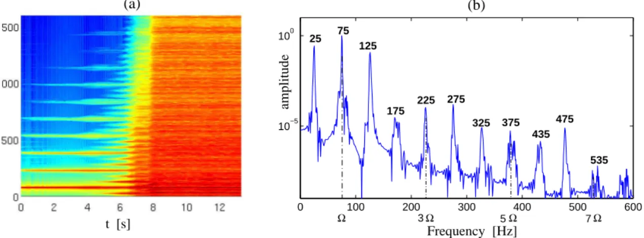
0 100 200 300 400 500 600 10−5 100 3Ω 5Ω 7Ω 25 75 125 175 275 225 325 375 435 475 535 Ω t [s] Frequency [Hz] Frequency [Hz] amplitude (b) (a)
Figure 6: (a): Spectrogram of output displacement wout for the plate excited at 75 Hz, with a forcing amplitude F from 0 to 28 N in 14 seconds. A superharmonic resonance is excited with participation of the first mode locked at 25 Hz from t=5 s, then the turbulent regime is obtained at t=8 s, i.e. for F=16 N. (b): Fourier transform of a 1.3 sec (Hanning window of 216=65536 points) computed at t=6 s showing
the spectral content of the vibration in the coupled superharmonic regime.
The first particular case studied is represented in Figure 6, observed for fexc=75 Hz, i.e. in
the vicinity of the fourth mode of the plate. The amplitude of the forcing is increased linearly from 0 to 28 N in 14 seconds. The first regime is the moderately non-linear regime where only the directly excited mode participates in the plate response. At t=5 s, a bifurcation is observed with the clear appearance of a frequency of 25 Hz in the vibration, as highlighted in Fig. 6(b). This frequency peak is the signature of the first eigenmode participation through a superhar-monic 1:3 resonance. It occurs for a non-negligible forcing amplitude (10 N), mainly because the 1:3 resonance relationship is not perfectly satisfied. Hence the 1:3 resonance relationship can be satisfied only for an energy that is sufficient so as to obtain a frequency shift of the first mode. The fact that internal resonance can occur between modes that are not commensurate natural frequencies has already been observed in [46, 47, 48, 49]. When increasing amplitudes of vibrations and thus the total energy level, periodic solutions follow nonlinear normal mode (NNM) branches, showing large variations of frequencies. Thus internal resonances can be ful-filled between the shifted frequencies, so that the examination of natural frequencies to predict possible mode coupling is not enough. A correct representation is to compute the variations of all eigenfrequencies as a function of the total energy of the system, resulting in a so-called Frequency-Energy Plot (FEP) [50]. The numerical result obtained here for fexc=75 Hz seems to
verify this kind of behaviour and resembles the results shown in [48] on a simple two degrees-of-freedom (dofs) system. This assumption could be fully confirmed by computing the complete FEP of the plate for the first frequencies, which is out of the scope of the present study. Once activation of the 1:3 superharmonic resonance is realized, the spectrum, shown in Fig. 6(b), is
logically composed of peaks being separated by 75-25= 50 Hz. However, one can observe that the third peak at 125 Hz is proeminent as compared to the followings, as it has almost equal energy than the spectral component at 25 Hz. As the seventh mode of the plate is given at 121.5 Hz, a possible assumption here is that this mode is also excited via energy transfer so that a 3-modes dynamics is present after the first bifurcation. The coupled regime persists during 4 seconds and is enriched in spectral content with an increase of the width of the spectral peaks, until the turbulent regime sets in for a forcing amplitude of F=16 N.
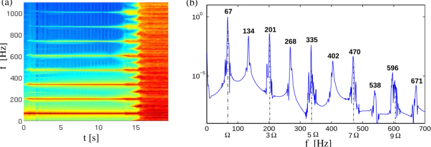
0 100 200 300 400 500 600 700 10−5 100 3Ω 5Ω 7Ω 9Ω Ω 67 134 201 268 335 402 470 538 596 671 f [Hz] t [s] f [Hz] (a) (b)
Figure 7:(a): Spectrogram of output vibration woutfor the plate excited at 67 Hz, with a forcing amplitude
F from 0 to 50 N in 20 seconds. A symmetry-breaking (SB) bifurcation is observed with the appearance
of even harmonics in the response, before the turbulent regime. (b): Fourier transform of a 1.3 sec segment (Hanning window of 216=65536 points) computed at t=14.5 s showing the spectral content of
the vibration after the SB bifurcation.
Surprisingly enough, the 1:3 superharmonic resonance has not been observed in the vicinity of the third mode, the eigenfrequency of which more closely fulfills the 1:3 ratio needed. This is confirmed in Fig. 7 where the scenario for fexc=67 Hz is shown. For this frequency, the
1:3 resonance is not excited, and a symmetry-breaking (SB) bifurcation is observed, which is characterized by the appearance of even harmonics in the response before the turbulent regime and a wideband Fourier spectrum. The SB bifurcation is classically observed in the Duffing equation, its location in the plane being, in frequency, between the 1:3 superharmonic and the main resonance; see e.g. [51, 52]. It has also been observed in the FEP of the two dofs system analyzed in [48, 49], where it was found to appear before the 1:3 internal resonance, what also seems to be observed here in the case of the plate. Once again, a complete picture of the internal resonance must include the energy level, so that a FEP should fully confirm the assumptions for the mode coupling observed here for fexc=75 Hz and fexc=67 Hz.
Finally, two other numerical experiments have been conducted in this frequency range, fexc=65 Hz and 70 Hz. For fexc=65 Hz, neither the SB bifurcation is found, nor the
super-harmonic resonance. Instead, a short quasiperiodic regime sets in with a clear appearance of frequency peaks at 25 Hz, 105 Hz and 155 Hz between the excitation frequency and the third harmonic at 195 Hz. These five frequencies fulfill third-order relationships so that an energy transfer is at hand. However, apart from the first frequency at 25 Hz that can be easily related to the first mode, it appears to be more difficult to relate the two new frequencies at 105 and 155 Hz to an eigenfrequency. Noting that the first regime is destabilized at a high value of
the forcing (around 50 N) for fexc=65 Hz, one can conclude that the frequencies have already
encountered a large variation due to nonlinearity. In the last test with fexc=70 Hz, a direct
transi-tion is obtained, highlighting that the internal resonance relatransi-tionships exist on narrow frequency intervals. 0 100 200 300 400 500 600 700 800 10−5 100 0 100 200 300 400 500 600 700 800 10−5 100 t [s] f [Hz] f [Hz] f [Hz] (a) (b) (c)
Figure 8: (a): Spectrogram of the output vibration wout for the plate excited at 130 Hz, with a forcing amplitude F from 0 to 30 N in 10 seconds. A direct transition is observed with frequency peaks of increasing width just before the turbulent regime. (b) and (c) : Fourier transforms of a 1.3 sec segment computed respectively at t=5 s and t=8 s.
The last case shown for the low frequency range is represented in Fig. 8, for fexc=130 Hz.
A similar behaviour has also been found for fexc=127 Hz and 142 Hz. Here the peculiar feature
is a marked broadening of the spectral peaks around all harmonics just before the turbulent regime, as illustrated in the two spectra of the output displacement wout shown in Fig. 8(b-c).
The interpretation of this bifurcation is not straightforward in this case, as it appears slightly different from a direct transition, but it could also be seen as a quasiperiodic state involving so many modes that peak identification is difficult. We note also that this spectral enlargement is one of the characteristics of modulation instability [53, 54, 55], which could be the correct interpretation in these cases. It is worth noting that these kinds of transitions have also been observed experimentally. Further research specifically concentrated on this case is however needed to ensure the category in which it falls. In the remainder of the article, this type of scenario will be called, for lack of a better term, modulation instability; at this stage it is simply a blanket term for a phenomenon that needs a more complete characterization.
3.4. High frequency excitation
In this section we discuss the results obtained in the frequency range [167, 342] Hz, here called the ”high frequency range” because the observed scenario differs radically from the cases discussed in the previous section. 15 numerical experiments have been conducted, and only two direct transitions without quasiperiodic regime have been found, whereas ten cases of energy transfer within the quasiperiodic regime have been observed, and three cases corresponding to the more difficult case shown previously with fexc=130 Hz and called modulation instability.
The tested frequencies are (in parenthesis the case obeserved: D for direct transition, QP for quasiperiodic regime, MI for Modulation instability, as well as the critical force amplitude ¯Acr
(QP, 31 N), 184 Hz (QP, 37 N), 190 Hz (QP, 21 N), 195 Hz (QP, 24 N), 198 Hz (QP, 66 N), 202 Hz (D, 19 N), 227 Hz (MI, 82 N), 230 Hz (QP, 100 N), 247 Hz (MI, 18 N), 300 Hz (QP, 42 N), 302 Hz (QP, 40 N), 304 Hz (QP, 20 N), 342 Hz (D, 50 N). Hence the dominant observed scenario is that of the appearance of the quasiperiodic regime, which will now be further highlighted. It is explained by the fact that exciting the plate at a higher frequency with numerous eigenmodes before the excitation frequency renders possible a larger number of resonance relationships, hence making this scenario more likely to appear. Three cases are shown and discussed.
0 200 400 600 800 1000 10−5 100 0 5 10 15 20 25 30 −1 0 1x 10 −3 0 100 200 300 400 500 600 700 10−5 100 f f t [s] t [s] f [Hz] w [m] (a) (b) f [Hz] (c) : FFT 1 (d): FFT2 FFT 1 FFT 2 f f f f f f f [Hz] f f f f f f f f f f 1 1 28 69 126 167 265 306 362 403 501 599 640 2 4 5 6 7 9 2 4 5 6 7 9 3 exc exc exc 3 exc
Figure 9:Transition scenario to turbulence for the perfect plate excited at 167 Hz, with a forcing amplitude from 0 to 65 N in 30 seconds. (a) : time series of the output displacement wout. (b) : spectrogram of the
vibration. (c) and (d) : Fourier transforms of 1.3 s of the displacement, respectively at t=7.5 s (c), and t=23 s (d).
The first case is that of the excitation frequency fexc=167 Hz, in the vicinity of the tenth
mode, depicted in Fig. 9, where the amplitude of the forcing ¯A is increased from 0 to 65 N in 30 seconds. A first bifurcation is observed at t=7.5 s, leading to a transient regime that fail to stabilize and lasts 5 seconds. This unstable transient regime is characterized by an increased width of the spectral peaks of the forcing harmonics, as shown in the first spectrum in Fig. 9(c). Then the stable quasiperiodic regime sets in, with a clear appearance of distinct frequency peaks shown in Fig. 9(d). For a better identification, the most prominent frequency peaks are denoted as: f1 = 28 Hz, f2 = 69 Hz, f3 = fexc = 167 Hz, f4 = 265 Hz, f5 = 306 Hz, f6 = 362 Hz, f7 = 403 Hz, f8 = 3 fexc = 501 Hz and f9 = 599 Hz. All of these new frequencies share evident
order-three internal resonances amongst themselves, highlighting the fact that energy has been transferred in order to arrive at the quasiperiodic regime. For most of them, they can also be easily identified to eigenfrequencies of the plate. From the order of appearance and respective magnitude of these peaks, the following scenarios can be identified. The first frequencies to appear, f2, f4, f7 and f9 are related to the excitation frequency f3 = fexc by the following
relationships:
f3 = f7− f2− f3, (25a)
f3= f9− f4− f3. (25b)
Moreover, f2, f4, f7 and f9 are near eigenfrequencies, respectively to modes number 3, 17, 26
and 41. Hence a first double order-three internal resonance is excited leading to a quasiperiodic regime with 5 modes exchanging energy. This 5-modes dynamics is rapidly destabilized for a more complicated regime including more modes, corresponding to all the frequency peaks identified in Fig. 9. These new frequencies appear with a little delay as compared to the first four identified, but they also share evident order-three relationships:
f3= f4+ f7− f8, (26a)
f3= f6+ f5− f8, (26b)
f3= f1+ f8− f6. (26c)
Eventually, the quasiperiodic regime involves 9 modes excited through energy transfers. The last bifurcation involves destabilization of this complicated 9-modes dynamics in favour of the turbulent regime. 19 20 21 22 23 24 25 26 −2 0 2x 10 −3 0 200 400 600 800 1000 10−10 10−5 100 0 200 400 600 800 1000 10−5 100 t [s] t [s] f [Hz] w [m] f [Hz] f [Hz] f1 f f4 f5f6 f7 f8 2 f2 f3 f7 f8 f1 f4 f5 f6 f3 20 87.5 195 370 410 477.5 585 692.5 302.5 31 81.6 148 195 310 425 585 = fexc = 3fexc FFT 1 FFT 2 (a) (b) (c) : FFT 1 (d) : FFT 2
Figure 10: Transition scenario to turbulence for the perfect plate excited at 195 Hz, with a forcing am-plitude from 0 to 35 N in 30 seconds. (a) : time series of the output displacement wout, zoom on the
transition between 19 and 26 s. (b) : spectrogram of the vibration. (c) and (d) : Fourier transforms of 0.65 s of the displacement, respectively at t=20 s (c), and t=21.1 s (d).
The second case selected for analysis is shown in Fig. 10, and corresponds to an excitation frequency of fexc= 195 Hz, in the vicinity of the 12th eigenfrequency. The forcing amplitude
Fig. 10(b), shows a clear scenario with a quasiperiodic state before the turbulent regime. The quasiperiodic state sets in progressively with the appearance of the following frequency peaks, identified in Fig. 10(b-c) : f1= 20 Hz, f2= 87.5 Hz, f3 = fexc= 195 Hz, f4= 302.5 Hz, f5= 370
Hz, f6 = 410 Hz, f7 = 477.5 Hz, f8 = 3 fexc = 585 Hz. The first step involves energy transfers
between f2 (in the vicinity of mode 5), f4 (mode 20), f7 (mode 32). The energy, injected on
f3 = fexc = 195 Hz spread to these new frequency peaks appearing first in the spectrogram
through the following order-three internal resonance relationships:
2 f3 = f2+ f4= f7− f2. (27)
Then, as shown in the displacement spectrum in Fig. 10(c), a new set of frequencies is excited through new internal resonance relationships. They appear later in the spectrogram with a smaller amplitude, indicating that the first identified resonance dominates. These new peaks, f1, f5and f6are not directly related to the excitation frequency f3 = fexc or its third harmonics,
so that their appearance is conditioned by the fact that the first step has been excited and that energy is present in f2, f4and/or f7. This second instability is characterized by energy transfers
through the following identified relationships:
f3 = f1+ 2 f2, (28a)
f4 = f1+ f2+ f3, (28b)
f5= f4+ f2− f1, (28c)
f6= f4+ f2+ f1, (28d)
f7= f2+ f1+ f5. (28e)
After this second instability, the quasiperiodic regime involves 8 modes. It is quickly destabi-lized in favour of the turbulent regime which sets in rapidly. Interestingly, once the turbulent regime is attained, energy is redistributed through all the lengthscales, so that the most promi-nent peaks, identified in Fig. 10(d), are distinct from the ones identified in the quasiperiodic regime, where the frequencies were locked to fulfill internal resonance relationships.
The last case analyzed is shown in Fig. 11, for fexc= 230 Hz, with a forcing amplitude
increasing from 0 to 110 N in 20 seconds. Once again a clear quasiperiodic regime sets in before the turbulent behaviour, hence recovering the general transition scenario inferred from the experimental measurements. The quasiperiodic state is much more complicated in this case with the appearance of 5 frequencies under the excitation frequency. All the frequency peaks share order-three internal resonance relationships, and there is a gap of 40 Hz between the majority of them.
Finally, all other excitation frequencies tested in this ”high frequency” range show a similar behaviour to that observed in the three cases illustrated. Consequently the generic transition scenario is fully confirmed by these numerical experiments. We now turn to an imperfect plate to simulate a more realistic case, because in experiments imperfections are unavoidable and order-two internal resonances in the quasiperiodic regime are always observed.
4. Simulation results for the imperfect plate 4.1. Selected case
The case of an imperfect plate is now studied by imposing a static deflection w0(x, y) to the
mid-plane of the plate having the form of a raised cosine: w0(x, y) = 1 2Aimp 1 + cos πp(x − x0)2+ (y − y0)2 Limp ; (29)
0 250 500 750 10−8 10−6 10−4 10−2 100 30 70 110 150 190 230 270 310 350 390 430 489 570 609 650 660 690 730 t [s] f [Hz] f [Hz] (a) (b)
Figure 11:(a): Spectrogram of the vibration wout for the perfect plate excited at 230 Hz, with a forcing amplitude F from 0 to 110 N in 20 seconds. (b): Fourier transform of 1.3 sec of the displacement at t=15 s. 0 0.3 0.6 0 1 2 x 10⁻³ 0 0.2 0.4 0 1 2 x 10⁻³ 0 50 100 150 200 250 300 0 1 2 3 4 5x 10 −3 0 0.2 0.4 0 0.2 0.4 0.6 0 1 2 x 10⁻³ (c) (a) (b) Aimp Aimp w0 w0 w0 A imp x y x y [m] f [Hz]
Figure 12: (a): cross-section (in the x and y directions) of the imperfection of amplitude Aimp (in m)
considered for the plate. (b): three-dimensional view of the imperfect plate. (c) : eigenfrequencies (in Hz) for increasing values of Aimp.
where Aimpis the height (in m) of the imposed static deflection, and Limpits width. The
imper-fection is centered at (x0, y0), as is shown in Fig. 12(a,b) for x0 = Lx/2 and y0 = Ly/2 which
will be the case considered in the remainder of the study. All the other parameters (material parameters ρ, E and ν, size Lx, Ly and thickness h) are unchanged with respect to the preceding
case so as to illustrate a continuous deviation from the perfect case studied in preceding section. The width Limphas been set to 0.2 m.
A modal analysis can be conducted by considering the linear part of Eqs.(2):
ρh ¨¯w + D∆∆ ¯w = L( ¯w0, ¯F), (30a)
∆∆ ¯F = −EhL( ¯w, ¯w0), (30b)
The associated eigenproblem is solved by using the finite-difference operators introduced in section 2. For increasing values of the imperfection amplitude Aimpfrom 0 to 5 mm, the
(equal to the thickness) is chosen for the simulations. Table 4 gives the first 18 eigenfrequencies for this case, computed with fS=50 kHz (Nx=36, Ny=54), i.e. the sampling frequency used for
the dynamical simulations.
24.81 42.34 68.33 81.63 87.24 122.35 124.78 145.78 162.56
166.49 184.10 198.76 226.42 241.67 247.69 255.65 265.61 298.38
Table 4: Eigenfrequencies for the imperfect plate chosen for the simulations, computed with Nx=36, Ny=54 spatial
points ( fS=50 kHz). Dimensions are: Lx = 0.4m, Ly = 0.6m, h=1 mm, Aimp=1mm, Limp = 0.2 m, material
parameters are: E= 200 GPa, ν=0.3 and ρ=7860 kg.m−3.
4.2. Transition scenario
As compared to the perfect plate, the distinction between low and high frequencies does not appear in the simulations conducted. This appears naturally as a reflection of the fact that adding quadratic nonlinearity enables more simple order-two internal resonance relationships so that the scenario with the quasiperiodic state appears for the very first frequencies. A set of 24 simulations has been conducted for fexc ranging from 25 Hz (second mode) to 202 Hz,
in the vicinity of the 12th mode (eigenfrequency at 199.25 Hz), i.e. in a somewhat narrower frequency band than for the perfect plate. The list of the frequencies tested (and in parenthesis the observed scenario: D for direct transition, QP for appearance of the quasiperiodic state (the resonance relationship is indicated when it was evident otherwise nothing is mentioned indicating that a single resonance could not be identified), MI for the last case where the direct transition is not clearly marked, as in the perfect case, as well as the critical force amplitude ¯Acr
(in N) for which the turbulent behaviour sets in) is: 26 Hz (D, 20 N), 42 Hz (D, 45 N), 70 Hz (D, 10 N), 81 Hz (D, 15 N), 84 Hz (QP, 8 N), 85.5 Hz (QP, 1:2 case, 10 N), 87 Hz (QP, 1:2, 11 N), 92 Hz (D, 20 N), 109 Hz (QP, 62 N), 111 Hz (D, 60 N), 120 Hz (D, 58 N), 123 Hz (MI, 54 N), 130 Hz (QP, 12 N), 137 Hz (MI, 24 N), 140 Hz (D, 25 N), 142 Hz (D, 21 N), 147 Hz (MI, 10 N), 150 Hz (QP, 22 N), 160 Hz (QP, 1+1:2, 46 N), 162 Hz (QP, 44 N), 164 Hz (QP, 42 N), 167 Hz (QP, 45 N), 180 Hz (QP, 1:2, 35 N), 202 Hz (MI, 14 N). Hence in the 24 simulations run, only 9 direct transitions are observed, which is markedly in contrast with the perfect plate. It is thus concluded that the presence of quadratic nonlinearity favours the mode coupling and the appearance of energy exchange leading to a quasiperiodic state, which can be more easily degenerated in this case due to occurrences of 1:2 resonance.
Fig. 13 shows the simulation results obtained for fexc=85.5 Hz. The 1:2 internal resonance
is activated for very small values of the forcing amplitude. The coupling is with the second mode, the eigenfrequency of which is 42 Hz. One may also note the appearance of all even har-monics of the forcing frequency, in accordance with the presence of the quadratic nonlinearity. The coupled regime where the two modes are present in the vibration persists until the forcing amplitude attains the value of ¯A= 12 N, a smaller value for obtaining the turbulent regime as compared to those observed for the perfect plate. This is in accordance with numerical results presented in [25].
A more complicated case is now analyzed for fexc=109 Hz, presented in Fig. 14. The
spectrogram and the Fourier spectrum of the displacement shown in Fig. 14(b) indicate that a first energy transfer follows from 1+1:2 internal resonance. The modes number 1 and 4, whose eigenfrequency are respectively 24.8 and 81.6 Hz, are excited and slightly shifted so as to perfectly fulfill the relationship f1+ f4 = fexc, with f1=26.3 Hz, and f4=82.7 Hz. The other
f [Hz]
t [s]
Figure 13: Spectrogram of output for the imperfect plate excited at 85.5 Hz, with a forcing amplitude F from 0 to 60 N in 20 seconds (with only the first 8 seconds shown). A clear 1:2 internal resonance is excited for F=4 N before the turbulent regime sets in for F=12 N.
0 100 200 300 10−6 10−4 10−2 100 f [Hz] t [s] (a) (b) f [Hz] = =
f
1f
2f
3f
5f
4f
6f
7f
8f
9f
10 218 191.9 165.6 161.6 135.4 109 82.7 56.4 52.3 26.3f
exc2 f
exc3f
excFigure 14:(a) Spectrogram of output for the imperfect plate excited at 109 Hz, with a forcing amplitude
F from 0 to 50 N in 20 seconds. (b) Fourier transform of 1.3 sec of the displacement wout at t=14 s, showing the combination resonances before the turbulent behaviour.
frequencies noted in the Fourier spectrum are denoted as: f2=52.3 Hz, f3=56.4 Hz, f5= fexc=109
Hz, f6=135.4 Hz, f7=161.6 Hz, f8=165.6 Hz, f9=191.9 Hz, f10=2 fexc=218 Hz. Inspecting
following order-two resonance relationships are fulfilled:
f1+ f3 = f4, (31a)
f1+ f8 = f9, (31b)
f3+ f7 = f10. (31c)
These three relations allows and explanation for energy transfer and the appearance of frequency peaks f3, f8, f9and f7. Finally f2and f6are not involved in any order-two relationships. Thus we
assume here that the presence of these frequency peaks is due to order-three internal resonance relationships, as one can verify that:
f2= f7+ f4− f9, (32a)
f6= f7+ f9− f10. (32b)
To conclude with this section, the distinction between low frequency and high frequency range for the imperfect plate has no meaning anymore since the generic transition scenario with the quasiperiodic state is the most frequently observed. The particular case of the perfect plate, unreachable in real experiments, enforces to make this distinction due to the lack of possible internal resonance that must mandatory be of order-three, and thus more difficult to activate. As soon as a small imperfection is considered (here equal to the thickness h), quadratic non-linearity is at hand, and energy transfer through quadratic couplings are more easily obtained. These numerical results confirms in particular that the imperfect plate is more likely to undergo instabilities for low levels of vibratory energy, as already shown in [25].
5. Turbulent behaviour 5.1. Wave Turbulence
In this section, we analyze the regime occurring after the second bifurcation and charac-terized by a broadband Fourier spectrum. Recently, theoretical and experimental studies have revealed that the correct framework for analysis is that of a weakly turbulent behaviour, cor-roborating preliminary experimental studies revealing the divergence of dimension calculations when using classical indicators of low-dimensional chaos [23, 13]. D¨uring et al apply the Wave Turbulence Theory (WTT) to von K´arm´an equations of motions governing the non linear dy-namics of thin plates, showing the existence of a direct cascade of energy through lengthscales and deriving their statistical properties in terms of energy repartition [26]. In particular, they show that the power spectrum Pw(k) for the displacement w, for a perfect plate, must verify the
following dependence: Pw(k) = C P1/3 [12(1 − ν2)]1/6 ln1/3(k⋆/k) pE/ρ k4 , (33)
where C is a constant, P is the injected power, and k = ||k|| the modulus of the two-dimensional wavenumber. Omitting the log-dependence that is neglectable before the k−4one, and translat-ing the theoretical prediction in the frequency domain and for the velocity ˙w, one obtains:
Pw˙( f ) =
C′P1/3h
[12(1 − ν2)]2/3f
0 (34)
where the term f0 has been written explicitly to underline the flat dependence as function of
discrepancy between theory and experiments that is attributed to the presence of damping, not taken into account in the theoretical derivations.
Here we want to compare the results of our simulations with the predictions provided by WTT. Consequently, an undamped plate is selected so as to verify the energy repartition of the power spectrum given by (34). Note that in [26], a numerical scheme based on a pseudospectral method has already been used to validate the theoretical prediction.
Figure 15 shows a snapshot of the transverse displacement w and velocity ˙w for the plate excited with an amplitude of ¯A=30 N and an excitation frequency of fexc= 87 Hz,
correspond-ing to Fig. 3. The spectrum of the displacement becorrespond-ing k-dependent as k−4, the snapshot of the displacement is quite smooth, while for the velocity higher frequencies are much more appre-ciable. This figure from numerical simulation can be compared to deformation and velocity measured experimentally and shown in [30].
x y x y w [m] w [m/s] (a) (b)
Figure 15:(a) Transverse displacement of the plate w(x, y) in the turbulent regime. (b) Transverse velocity ˙
w(x, y). The undamped plate is excited at fexc= 87 Hz with a forcing amplitude ¯A=30 N.
5.2. Power spectra
Numerical simulations of turbulent behaviour in conservative media are difficult because of the simultaneous presence of a cascade of energy (a priori infinite) from large to small length-scales and the absence of dissipation in the system. As the energy flux enforces the creation of smaller and smaller lengthscales, a numerical problem is encountered when the Nyquist fre-quency, being half the sampling frequency fS, is attained. From that, energy comes back into the
simulation box as it should normally go to smaller lengthscales that are not simulated. Hence conducting numerical simulations in the undamped case requires, a priori, a very high value of fS in order to have a frequency band of interest where the cascade develops without numerical
interference.
This is illustrated in Fig. 16, where the complete spectrograms of two simulations with the same set are shown, and for two different sampling frequency fS. The undamped plate (σ0 = 0)
is excited with fexc = 75 Hz, the amplitude of the forcing being increased from 0 to 80 N in two
seconds, then kept constant during 8 seconds and finally cut off until the end of the simulation. In Figs 16(a-c), the sampling frequency is fS= 100 kHz, while in Figs 16(b-d) it has been set
0 2 4 6 8 10 12 14 0 2 4 6 8x 10 7 0 5 10 15 0 2 4 6 8 10x 10 7 fc fc t [s] t [s] t [s] t [s] f [Hz] f [Hz] Energy Energy (a) (b) (c) (d) f = 400 kHz f = 100 kHzs s
Figure 16:Spectrograms and Energies for the undamped plate excited at fexc = 75 Hz. (a)-(c): fS = 100
kHz, (b)-(d): fS = 400 kHz. Bending energy in blue, in-plane energy in magenta, total energy in black.
exhibits a numerical cut-off, at: fC = fS π Arcsin 2κ fS (h2 x+ h2y) h2 xh2y (35)
In the limit of high sample rate, and if the grid spacings are chosen exactly according to the stability condition, this cutoff is precisely the Nyquist frequency fS/2; in practice, however,
there will be a slight loss of bandwidth due to a choice of grid spacings away from this bound (so, e.g., one may have the domain divided evenly into an integer number of grid points along each dimension).
For fS = 100 kHz, one can observe that the upper frequency generated by the cascade
quickly attains the Nyquist frequency. Due to the numerical limitation, the energy seems to be blocked in the very high frequency range, and starts to accumulate. Hence from that point, the computed solutions are not physical anymore, and what is observed is due to numerical limitations. This is also clearly seen on the energies. For fS = 100 kHz, on can see in Fig. 16(c)
that up to 5 seconds, the total energy increases linearly, the in-plane energy being maintained at a neglectable value. Then this in-plane energy starts to increase slowly and dramatically, with an evident broke-up in the slope of the total and bending energies. From that moment the numerical solutions are non physical anymore. What is observed is a sort of thermalization where the system relaxes to an absolute equilibrium state completely driven by the numerical limitation. Similar numerical observations are shown for Euler flows in turbulent regime [58].
For fS = 400 kHz, the time for the energy flux to generate an upper frequency attaining the