HAL Id: hal-01318124
https://hal.archives-ouvertes.fr/hal-01318124
Submitted on 19 May 2016
HAL is a multi-disciplinary open access
archive for the deposit and dissemination of
sci-entific research documents, whether they are
pub-lished or not. The documents may come from
teaching and research institutions in France or
abroad, or from public or private research centers.
L’archive ouverte pluridisciplinaire HAL, est
destinée au dépôt et à la diffusion de documents
scientifiques de niveau recherche, publiés ou non,
émanant des établissements d’enseignement et de
recherche français ou étrangers, des laboratoires
publics ou privés.
Tuning interpolation methods for environmental
uni-dimensional (transect) surveys
You Li, Maria-João Rendas
To cite this version:
You Li, Maria-João Rendas. Tuning interpolation methods for environmental uni-dimensional
(tran-sect) surveys. OCEANS 2015, IEES OES, Oct 2015, Washington DC, United States. �hal-01318124�
Tuning interpolation methods for environmental
uni-dimensional (transect) surveys
You Li and Maria-Jo˜ao Rendas
Laboratoire I3S, CNRS Sophia Antipolis, FRANCE Email:{yli}{rendas}@unice.fr
Abstract—The paper proposes rCV, a new randomised Cross
Validation (CV) criterion specially designed for use with data acquired over non-uniformly scattered designs, like the linear transect surveys typical in environmental observation. The new criterion enables a robust parameterisation of interpolation algorithms, in a manner completely driven by the data and free of any modelling assumptions. The new CV method randomly chooses the hold-out sets such that they reflect, statistically, the geometry of the design with respect to the unobserved points of the area where the observations are to be extrapolated, minimising biases due to the particular geometry of the designs. Numerical results on both simulated and realistic datasets show its robustness and superiority, leading to interpolated fields with smaller error.
I. INTRODUCTION
Environmental observation of an extended regionA is often accomplished by using a motorised platform equipped of sensing equipment that performs a trajectory p(·) ⊂ A that “covers”A with a series of nearly paralell line transects. The trajectory followed by a surface boat during observation of a lake in Belgium shown in Figure 11 is a representative
example. Sensor acquisition rate and carrier speed, along with limitations in power and time, result in a much higher sampling rate along the trajectory of the carrier than the average point density overA. This apparent in Figure 1, that actually plots (color coded) the individual sampled values.
The ultimate goal of spatial surveys is to produce a map of some observed field f (·) over the entire region A, i.e., to extrapolate (the term ”predict” is also used) the point samples of f (·) taken along the carrier path to the entire surface.
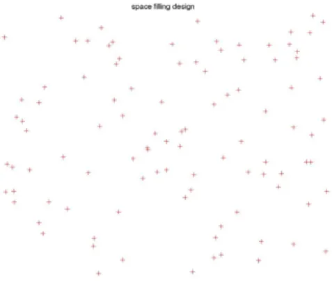
In this paper we address the problem of tuning the param-eters of the algorithm used to estimate the value of f (·) at the unobserved points of A, taking into account that the set of sampled points (the design) may have an arbitrary geom-etry, in particular the intrinsically one-dimensional geometry described above. A method widely used by practitioners to chose algorithm’s parameters is Cross Validation (CV), whose origins go at least as far as the 1930’s, see the interesting discussion in [1]. As we show below, CV works well in the geo-statistical context when the data points are “space filling”, i.e., uniformly scattered in A, as in Figure 2. This is clearly not the case for the uni-dimensional design of Figure 1. This paper presents rCV, a novel randomised version of CV
1Courtesy of VITO.
Fig. 1. Design used for a lake observation (courtesy of VITO).
specially tailored to be robust with respect to strongly “non space filling” design geometries.
Fig. 2. Space filling design.
We start by introducing notation and formulating the algo-rithm tuning problem (section II) and subsequently present CV methodologies (section III) pointing out the specific difficulties that arise for uni-dimensional designs. Section IV presents rCV, the new randomised CV method that we propose. Finally, we demonstrate (section V) the advantages of rCV in both
real and simulated datasets, and section VI summarises our contribution and lists some directions for future work.
II. PROBLEM FORMULATION
Let Y(K) denote the complete set of measures acquired during a one-dimensional survey done along path p(·) ⊂ A
Y(K)={yk = f (p(ℓk)) , k = 1, . . . , K}
Let Ξ be the design, i.e., the set of points at which observations are made
Ξ ={p(ℓk), k = 1, . . . , K} ,
and denote by ξk = p(ℓk) a generic point of Ξ.
Let F denote the operator that when applied to the set of measures Y(K) generates the field predictions (the extrapola-tion algorithm): ˆ f (s|Y(K); ρ) = F ( s, Y(K); ρ ) , s∈ A . As indicated above, F usually depends on a series of pa-rameters ρ ∈ Rq (for instance, the kernel scale and trend model for kriging methods, or the number of neighbours or neighbourhood size in local regression methods) that must be defined by the user. Choice of ρ is particularly important when, as it is often the case in environmental applications, Ξ does not sampleA densely.
Several criteria can be used to measure the quality of spatial extrapolation. We consider here the most common one, the Integrated Square Error (ISE), even if the method proposed is independent of this particular choice:
Cise(ρ; Y(K)) = 1 |A| ∫ A e2ρ(s; Y(K)) ds, (1) eρ(s; Y(K)) = f (s)− ˆf (s|Y(K); ρ) .
Ideally, one would choose ρ such that the reconstruction error is minimal:
ρ⋆(Y(K)) = arg min
ρ
Cise(ρ; Y(K)) . (2)
Note that Cise cannot be computed, as it depends on the
field’s values outside the design Ξ, and only estimates of Cise
based on the available data Y(K) can be used to chose ρ.
Two different frameworks are envisageable: (a) a parametric stochastic modelM(γ) is known to capture the characteristics of the field f (·) , enabling determination of the expected value of Cise; (b) Cisemust be estimated using only Y(K), no
addi-tional knowledge about f (·) being available. Kriging methods fall under (a), the interpolation algorithm being intrinsincally tied to a stochastic model of the observed field: data Y(K) can be used to estimate the model parameters ˆγ(Y(K)), which
determine the optimal (in an expected value sense) estimator of f (·) at unobserved points of A. Model-based frameworks are sensitive to the correctness of the assumed models, and for this reason (b) is often the preferred practitioners’ choice. In this paper we propose a new estimator of the reconstruction errror for subsequent selection of the value of ρ using Cross Validation, a popular methodology belonging to framework (b), see the section below.
III. CROSSVALIDATION
Several variants of CV exist [2], but the simple description below captures the main principle at work behind them all and is sufficient for the purpose of this paper.
Let ξi denote a generic point of Ξ, Ξ(−i) a subset of Ξ that
does not contain ξi and Y−(i) the corresponding measures.
A realisation of the interpolation error for algorithm F with parameters ρ is obtained by using Y(−i) to estimate the field at ξi:
ϵρ(ξi; Y(−i)) = yi− ˆf (ξi|Y(−i); ρ), ξi∈ Ξ .
Averaging these residuals over ξi ∈ Ξ yields a CV estimate
of Cise CCV(ρ|Y(K)) = dCise(ρ|Y(K)) = 1 |Ξ| ∑ ξi∈Ξ ϵ2ρ(ξi; Y(−i)) , (3) that can be used to select ρ by ρ⋆= arg min
ρCCV(ρ|Y(K)).
Different choices for the sets Y(−i) give rise to different
variants of CV, the most common being “leave-one-out,” where Y(−i)= Y(K)\ {y
i}.
As it is obvious from the presentation above, one necessary condition for CCV(ρ|Y(K)) to be a sensible estimate of
the true error is that the set of “cross-validation residuals” ϵρ(ξi; Y(−i)) be a representative sample of the prediction error
process at unobserved points of A. This is never exactly the case, and in fact one can show that CCV is in general a
con-servative estimate of the error, i.e., it predicts a performance poorer than the expected one, and several corrections have been proposed to eliminate this negative bias. However, it is customarily accepted that this bias it does not affect the location of the minimum of CCV as a function of ρ, i.e., the
uncorrected CV criterion can safely be used to select the best interpolating model.
Let us now analyse the impact of the one-dimensional design geometry on the quality of CCV as an estimator of
the true prediction error.
Spatial interpolation is known to be particularly sensitive to the geometry of Ξ around each reconstructed point. An additional condition for the validity of CCV as a proxy of the
interpolation error Ciseis thus that, around each design point
ξi, the geometry of the designs Ξ(−i) be representative of the
spatial distribution of the points of Ξ around generic unob-served points ofA. This is true for “space filling designs”2,
where the density of the design points is nearly homogeneous insideA, but is violated in the case of uni-dimensional surveys as the ones considered in this paper.
Consider the extreme case of the leave-one-out CV, where Y(−i)= Y(K)\ {y
i}, that clearly reveals the biasing effect of
uni-dimensional designs Ξ. Points of Ξ are naturally numbered along the curve p(·). There are two nearest neighboors in the sets Ξ(−i), for each ξ
i: ξi−1 and ξi+1, at distances d− =
∥ξi−ξi−1∥ ≃ d+=∥ξi−ξi+1∥. The estimates at ξiproduced
2The exact definition of ”space filling” varies in the literature, but here it is
sufficient to say that points of these designs are as far away from each other as possible.
by most interpolation algorithms will be strongly determined by these two points, with an error that will be small if these distances are small, i.e., when p(·) is densely sampled, as we consider in this paper.
To facilitate analysis, consider the simple case of a regular survey with transects of length L spaced D apart. The dis-tribution of distances of a generic points s ∈ A to Ξ can be approximated by πΞ(d)≃ ( 1 + D 2L− 2 Ld ) , d∈ [ 0,D 2 ] , which, for D ≪ L is close to the uniform distribution in [0,D2]. With probability ≃ 1 − 2δ+/D the distance of points
in A to Ξ will be larger than d− ≃ d+, the distance to the
closest points in the leave-one-out hold sets Y(−i), leading
to largely optimistic CV estimates of the reconstruction error, i.e., the CV criterion (3) will be much smaller than the actual reconstruction error (1).
For model-based estimators, if the model assumed is correct, the minimum of CCV(·) can still occur, in average, near the
”good value” of parameter ρ, as our results on simulated data in section V show. However, in the most likely situation that the observations do not follow the model for which F has been designed, standard CV criteria will be unable to capture the behaviour of the prediction error over the entire range of possible situations (in terms of distances to the closest data points). The randomised CV method presented in the next section overcomes this limitation.
IV. RANDOMISEDCROSSVALIDATION(RCV) As mentioned in the previous section the reconstruction error at a point s ∈ A is highly dependent on the local geometry of the points of Ξ in the neighborhood of s. In a first order approach this error is dominated by the distance of s to its closest point in Ξ, see [3]. This justifies use of the common minimax design criterion that minimises CmM(Ξ),
the maximum distance between points ofA and the design Ξ: CmM(Ξ) = max
s∈Aminξ∈Ξ∥s − ξ∥ .
This criterion is difficult to compute, requiring a search over the entire regionA, and the maximim criterion CM mis often
used instead. It evaluates a design by the distance between the closest points of Ξ, which should be as large as possible:
CM m(Ξ) = min ξ1,ξ2∈Ξ
∥ξ1− ξ2∥ .
Maximising this criterion leads to maximally spreading all points inside A, and is known to push some of the design points to its boundary, which is certainly not optimal from the point of view of the CmM criterion. For designs with good
space filling properties the set of distances {d(ξi, Ξ(−i)), ξ∈
Ξ} is expected to be a typical sample from the distribution of distances{d(s, Ξ), s ∈ A}, which is a condition for (3) to yield a valid indication of (1).
It is obvious that dense one-dimensional transect designs like the ones considered in this paper are not space filling
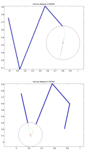
Fig. 3. Example of block-out sets Y−(s,r)
under any purely geometric criterion. When Ξ is a regular sampling of a one-dimensional curve p(ℓ), CM m will be
trivially equal to the distance between adjacent points, while CmM will most likely be equal to D/2 as the approximate
expression for πΞ given above shows. That the difference
between CM nand CmM is large is an indication that standard
CV techniques will fail to provide a valid indication of the expected performance when extrapolating over the entireA.
Let d(s, Ξ) be the distance between point s∈ A and Ξ: d(s, Ξ) = min
ξ∈Ξ∥s − ξ∥ ,
and, as before, let πΞ(d) the probability distribution of d(s, Ξ)
when s∼ U(A), i.e., when s is uniformly distributed in A. For any s∈ A and r ≥ 0 let Br(s) be the ball of radius r
centred at s, and denote by Ξ−(s,r) be the sets
Ξ−(s,r)= Ξ∩ Br(s)c , (4)
and denote by Y−(s,r) the corresponding measures. Notation Ac denotes complement of set A in A. Figure 3 illustrates
the definition of the sets Y−(s,r), the hold-out sets used in our randomised CV.
Randomised CV criterion
The randomised CV criterion for the prediction error over region A using observations Y(K) taken over design Ξ is
CrCV(ρ|Y(K)) = Er,ξ ( y(ξ)− F ( ξ, Y−(ξ,r), ρ ))2 , (5) where the statistical average is computed using distributions r ∼ πΞ and ξ ∼ U(Ξ), and the hold-out sets Y−(ξ,r) are
defined by (4).
Criterion CrCV, as equation (5) shows, uses randomly
chosen hold-out sets, that statistically reflect the geometry of design Ξ with respect to the entire regionA: it puts CV in the geometrical conditions under which extrapolation will actually be done.
The numerical computation of CrCV ressorts to stochastic
simulation, the expected value in the definition (5) being approximated by the empirical average
CrCV(ρ|Y(K))≃ 1 M M ∑ i=1 ( yi− F ( ξi, Y−(ξi,ri), ρ ))2 ,
where yi = y(ξi), M ∝ |A| is a large number and the pairs
(ξi, ri) are independently drawn according to
1) ξi∼ U(Ξ)
2) ri= d(si, Ξ), si ∼ U(A).
The price payed for the robustness of CrCV is its higher
numerical complexity: the number of criterion evaluations (predictions) is now of the order of the size ofA, usually much larger than the size of Ξ, required for instance by leave-one-out CV. Also, the determination of the distances d(si, Ξ), requiring
a minimisation over Ξ, are computationally expensive. Note that for designs based on paths p(·) ans sets A of simple geometry, for which πΞ can be approximated analytically,
computation of these distances can be avoided. V. NUMERICALRESULTS
We compare the performance of several sptatial interpola-tion methods tuned by the randomised CV proposed in the paper to the following methods.
1) Usual leave-one-out (LOOCV). This corresponds to using all other points to estimate each observation, i.e., to hold-out sets of the form
Ξ(−i) = Ξ\ {ξi} .
Comparison with this criterion will show the importance of holding out points close to the interpolation point. 2) Fixed distance hold-out (Fix). This is a simplified
ver-sion of rCV, and corresponds to considering hold-out sets which are of the form
Ξ(−i)= Ξ−(ξi,r⋆) .
This is a standard approach used for correlated data, where the value of r⋆ is specified by the user, based
on its expectation with respect to the field’s correlation range, which in general is unknown. We propose instead
to adjust the hold-out distance r⋆ based on the distribu-tion πΞ, and set r⋆to a fixed quantile α of πΞ, i.e., such
that
Prob{d(s, Ξ) ≤ r⋆} = α .
We used α = .75 in the numerical results below. Comparison with this criterion will enable us to assess the importance of using hold-out sets that reflect πΞ(d),
even if in a simplified manner.
3) Variogram (Var). To stress the robustness of the pro-posed criterion, we also show numerical results for Kriging, comparing the observed prediction errors of the optimal Kriging estimator using a range parameter ρ chosen by CrCV to the standard use of variogram
considered by most geo-statistics packages. A. Simulated Data
This section considers simulated datasets which are reali-sations of a Gaussian Process (GP) of zero mean and Mat´ern correlation function with parameter ν = 3/2
R(s, s′) = σ2 ( 1 + √ 3∥s − s′∥ ρ ) exp ( − √ 3∥s − s′∥ ρ ) , with ρ = 10. The field is simulated inside a square region A = [0, 60] × [0, 60]. Figure 6 shows one of the simulated fields and the one-dimensional design used in the numerical results shown below.
Interpolation by both non-parametric (Local Weighted re-gression, LWR) and parametric (Kriging) methods are studied. 1) LWR: is a common interpolation method that fits simple local parametric models f (s) = F (s; θ(s, ρ)) to the dataset. At each point s ∈ A, the parameters θ(s, ρ) minimise the weighted average θ(s, ρ) = arg min θ ∑ yi∈Y(K) w(s, ξi; ρ) (yi− F (s; θ)) 2 ,
where the weights w(s, ξi; ρ) are a decreasing function of
∥s − ξi∥ such that
∑
i
w(s, i; ρ) = 1 .
The local models that are fit are most commonly of polynomial type, θ being the coefficients of these polynomials. The original method [4] considers weighting functions of compact support, the parameter ρ being the size of this support, making at each point a truly local (weighted) fit to a strict subset of Y(K). Alternatively, we may consider functions of infinite support, like exponential or Gauss functions, and in this case ρ controls the speed with each the w(s,·; ρ) tends to zero. The numerical results below use a Gauss weight function.
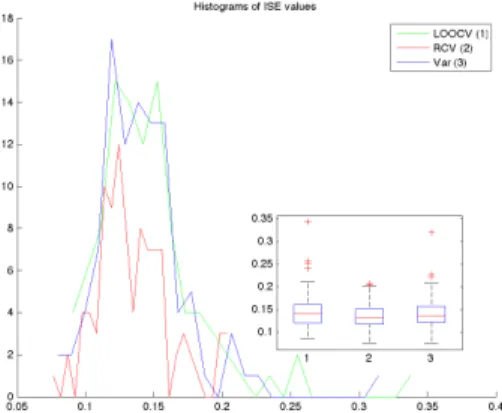
Figures 4 and 5 illustrate the performances observed in 100 distinct simulations of the model above for quadratic LWR. The three tuning methods studied here are LOOCV (green), rCV (red) and the fixed-distance hold-out set (blue). We also plot (black curve) the ISE values for the best ρ parameter that can be adjusted to each of the 100 simulated datasets.
Fig. 4. ISE for LWR using different tuning methods (one-dimensional design).
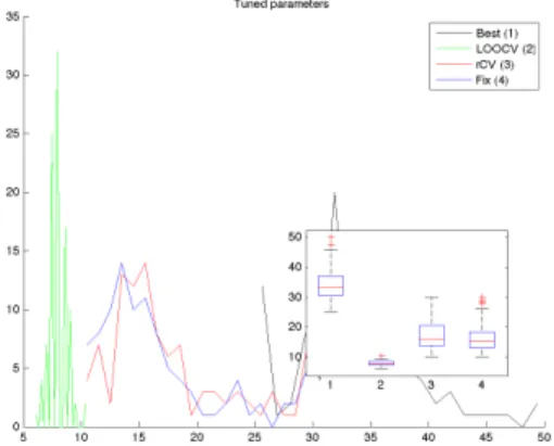
Fig. 5. Tuned LWR parameters (uni-dimensional design).
We can see that rCV consistently leads to better interpolation performance (lowest ISE), see Figure 4. Average values of ISE are equal to 0.186 for LOOCV, 0.131 for rCV and 0.135 for fixed hold-out. The actual minimum of ISE (computed using knowledge of the entire simulated field) is equal to 0.101. As we see, even the simple hold-out sets using a fixed distance already lead to a good improvement over LOOCV, showing how important it is that the sets Ξ(−i) reflect the
actual geometric conditions under which the dataset will be interpolated. Figure 5 shows histograms and corresponding box-plots of the tuned parameters ρ (in this case the rate of the Gaussian weight function) for the 100 datasets. As it should be expected, the rate chosen by LOOCV is systematically lower than the rates chosen by the other two methods, leading to a worst performance when interpolating over distant points. The ”best” ρ parameters are also shown for comparison.
Figure 7 shows the interpolation results for one of the sampled fields using the parameters tuned by LOOCV (top) and rCV (bottom).
2) Kriging: Kriging [5] is a popular geo-statistical interpo-lation method that implements the optimal mean-square error estimate of a spatial field based on the assumption that it is a realisation of a stationary Gaussian Process. Several variants
Fig. 6. Simulated Gaussian field and one-dimensional design.
Fig. 7. LWR interpolated fields with weight rate chosen by LOOCV (top) and rCV (bottom). Compare with Figure 6.
Fig. 8. ISE values for Kriging, one-dimensional design.
of Kriging exist, considering different modelling approaches for the mean function of the process. Simple Kriging assumes a known mean, ordinary kriging a constant unknown mean, and universal Kriging assumes that the mean function of the process belongs to the linear span of a finite set of known functions, most commonly polynomials. The estimator is linear in the observations, and is fundamentally determined by the correlation function of the GP. In this paper we studied ordinary Kriging, considering tuning of the range parameter ρ of the Mat´ern covariance using the variogram, LOOCV and rCV.
Figure 8 plots the ISE observed for Kriging. It can be seen that the new criterion leads to slightly better tuning of the interpolation method, although impact is less in this case, since the observations are realisation of the assumed stochastic model: the average ISE over theses 100 realisation is 0.1454 for LOOCV, 0.1412 for the Variogram and 0.1351 for rCV, such that, again rCV leads to the best tuning.
Figure 9 shows the ISE for observations over a regular grid with the same number of points as the previous designs, showing that randomisation does not lead to ISE increase, even when its higher numerical complexity is not justified. In fact, although all three methods lead approximately to the same performance, as it should be expected since in this case the inter-design distances reflect well what happens for generic points ofA. Although the designs have the same size, remark the strong impact of design geometry on the absolute value of the prediction error.
Figures 10 and 11 show the values of ρ that were chosen by the different criteria. For the one-dimensional design (Figure reffig:line:rg) rCV and Var lead to the values of ρ closer to the true one, LOOCV seriously underestimates ρ, while for the regular design (Figure 11) CV is best able to identify the true model (although this does not map into a better ISE, as Figure 9 shows). The parameter estimates for the regular design shows similar performance of rCv and LOOC, underestimating the value of ρ, while the variogram is not significantly affected by the change of design geometry.
Fig. 9. Values of ISE for Kriging using, regular design.
Fig. 10. Values of ˆρ, Kriging, one-dimensional design.
TABLE I
ISE,INTERPOLATION OF FIELD INFIG. 12. LWR (linear) LWR (quad.) Kriging CV 0.007536 0.083414 0.003984 rCV 0.002778 0.003551 0.002887 fix 0.002947 0.008507 0.003746 Var ⋆ ⋆ 0.002961 TABLE II ρ,FIELD INFIG. 12.
LWR (linear) LWR (quad.) Kriging CV 2.5 10 3.3 rCV 10 26 8.6 fix 7.5 18 16.3 Var ⋆ ⋆ 9.43
B. Real Data
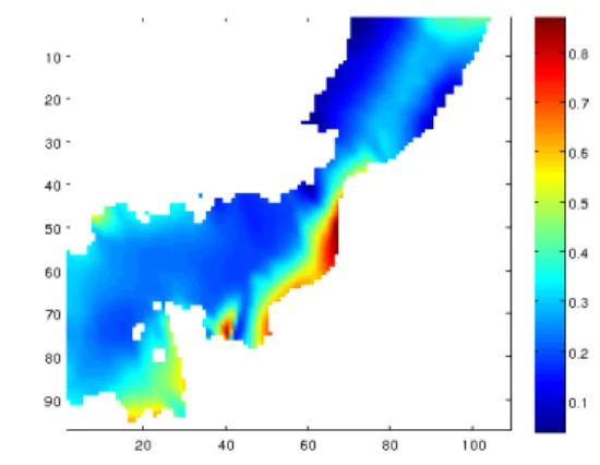
We also compare rCV to the other methods on a realistic dataset, produced by the MIRO&CO oceanographic model [6], that predicts the annual cycle of inorganic and organic carbon and nutrients, phytoplankton, bacteria and zooplankton under realistic forcing conditions. The model covers the entire water column of the Southern Bight of the North Sea. The scalar field used, see Figure 12, is Chlorophyllα. The uni-dimensional
survey trajectory that has been simulated is the thin black line in the Figure, that samples the field rather coarsely along a series of nearly parallel transects. Tables I and II summarise our results.
The tables show the ISE values and the identified parameters ρ for both linear and quadratic LWR and Kriging (using a Mat´ern covariance with ν = 3.2). For the Kriging estimator, use of the variogram has also been considered. We can see that rCV consistently leads to better interpolation performance for all interpolation methods. The global minimum being achieved for linear LWR, with an ISE value of 9.7 (the interpolated field is shown in 13, remark the large errors outside the convex hull of the design), and it is only slightly degraded for the other interpolation methods, being highest for quadratic LWR (ISE = 12.4). Compare with use of standard CV, that may lead to ISE values up to 291 (quadratic LWR). The fixed CV using πΞ is also consistently better than CV, but is less robust than
rCV, leading to an important degradation for quadratic LWR. The method that is the less sensitive to the tuning method is Kriging for which the ISE of all methods is in the interval [10.08, 13.91].
Analysis of the parameters identified, Table II, confirms that standard CV always leads to more local interpolation for this type of designs (smaller values of ρ).
VI. CONCLUSION
This paper presents a new Cross Validation Criterion in-tended to be used on datasets acquired along linear/transect surveys, a common practice in environmental observation. The new criterion is a randomised version of standard CV, where the hold-out sets are randomly chosen in order to statistical replicate the local geometry of the design around each point in
Fig. 12. Chlorophyllα field produced by model MIRO&CO (courtesy of
MUMM).
Fig. 13. Interpolated field (LWR with linear model, rCV tuning).
the target interpolation region. We formally motivated the new method, and illustrated its advantage with respect to standard CV (and even parametric moment-matching techniques like use of variogram in the context of kriging) in both simulated and realistic oceanographic data. Future work along the same line concerns two issues: (i) CrCV(·) makes sense only in
the context of prediction of spatially stationary fields, and we are studying how we can apply the same idea to enable local adjustment of the interpolator parameters, see [7]; (ii) the numerical complexity of Crev(·) is much higher than
standard CV, and two directions will be explored to improve its efficiency: (a) consider analytical approximations to πΞ(d),
as outlined in section III, eliminating the need to estimate πΞ;
(b) consider ”fast CV” approaches, that exploit the recursive version of some estimators.
ACKNOWLEDGMENTS
This work has been partially supported by the European Union through project DRONIC (FP7-ICT 611428, “Appli-cation of an unmanned surface vessel with ultrasonic, en-vironmentally friendly system to (map and) control blue-green algae (Cyanobacteria),” http://dronicproject.com/), and by ANR (France) through project DESIRE (https://www.i3s.
unice.fr/desire/). The authors acknowledge the collaboration of the Institutes VITO and MUMM (Royal Belgian Institute of Natural Sciences) in providing some of the datasets used in this work.
REFERENCES
[1] M. Stone, Cross-validatory Choice and Assessment of Statistical
Predic-tion, Journal of the Royal Statistical Society. Series B (Methodological),
Vol. 36, No. 2, pp. 111-147, 1974.
[2] S. Arlot, A Survey of Cross Validation Procedures for Model Selection, Statistics Surveys, Vol. 4, pp 40-79, 2010.
[3] L. Pronzato and W. Muller, Design of computer experiments: space filling
and beyond, Statistics and Computing, Springer Verlag (Germany), 22 (3),
pp.681-701, 2012.
[4] W. S. Cleveland and S. J. Devlin, Locally-Weighted Regression: An
Ap-proach to Regression Analysis by Local Fitting, Journal of the American
Statistical Association, vol. 83, no 403, p. 596610, 1988.
[5] C. E. Rassmussen, Gaussian processes for machine learning, MIT Press, 2006.
[6] G. Lacroix, K. Ruddick, Y. Park, N. Gypens, and C. Lancelot, C.,
Valida-tion of the 3D biogeochemical model MIRO&CO with field nutrient and phytoplankton data and MERIS-derived surface chlorophyll α images.,
Journal of Marine Systems, Vol 64, p. 66-88, 2007.
[7] G. Lacroix, K. Ruddick, Y. Park, N. Gypens, and C. Lancelot, C., Local
Polynomial Modelling and Its Applications: Monographs on Statistics and Applied Probability, Monographs on Statistics and Applied Probability