HAL Id: hal-02988148
https://hal.sorbonne-universite.fr/hal-02988148
Submitted on 4 Nov 2020
HAL is a multi-disciplinary open access
archive for the deposit and dissemination of
sci-entific research documents, whether they are
pub-lished or not. The documents may come from
teaching and research institutions in France or
abroad, or from public or private research centers.
L’archive ouverte pluridisciplinaire HAL, est
destinée au dépôt et à la diffusion de documents
scientifiques de niveau recherche, publiés ou non,
émanant des établissements d’enseignement et de
recherche français ou étrangers, des laboratoires
publics ou privés.
A semiclassical Thomas-Fermi model to tune the
metallicity of electrodes in molecular simulations
Laura Scalfi, Thomas Dufils, Kyle Reeves, Benjamin Rotenberg, Mathieu
Salanne
To cite this version:
Laura Scalfi, Thomas Dufils, Kyle Reeves, Benjamin Rotenberg, Mathieu Salanne. A
semiclassi-cal Thomas-Fermi model to tune the metallicity of electrodes in molecular simulations. Journal of
Chemical Physics, American Institute of Physics, 2020, 153 (17), pp.174704. �10.1063/5.0028232�.
�hal-02988148�
to tune the metallicity of electrodes in
molecular simulations
Cite as: J. Chem. Phys. 153, 174704 (2020); https://doi.org/10.1063/5.0028232
Submitted: 03 September 2020 . Accepted: 14 October 2020 . Published Online: 04 November 2020
Laura Scalfi, Thomas Dufils, Kyle G. Reeves, Benjamin Rotenberg, and Mathieu Salanne COLLECTIONS
This paper was selected as Featured This paper was selected as Scilight
The Journal
of Chemical Physics
ARTICLE scitation.org/journal/jcpA semiclassical Thomas–Fermi model to tune
the metallicity of electrodes in molecular
simulations
Cite as: J. Chem. Phys. 153, 174704 (2020);doi: 10.1063/5.0028232
Submitted: 3 September 2020 • Accepted: 14 October 2020 • Published Online: 4 November 2020
Laura Scalfi,1,2 Thomas Dufils,1,2 Kyle G. Reeves,1,2 Benjamin Rotenberg,1,2 and Mathieu Salanne1,2,3,a)
AFFILIATIONS
1Sorbonne Université, CNRS, Physico-chimie des Électrolytes et Nanosystèmes Interfaciaux, PHENIX, F-75005 Paris, France 2Réseau sur le Stockage Electrochimique de l’Energie (RS2E), FR CNRS 3459, 80039 Amiens Cedex, France
3Institut Universitaire de France (IUF), 75231 Paris Cedex 05, France
a)Author to whom correspondence should be addressed:mathieu.salanne@sorbonne-universite.fr
ABSTRACT
Spurred by the increasing needs in electrochemical energy storage devices, the electrode/electrolyte interface has received a lot of interest in recent years. Molecular dynamics simulations play a prominent role in this field since they provide a microscopic picture of the mechanisms involved. The current state-of-the-art consists of treating the electrode as a perfect conductor, precluding the possibility to analyze the effect of its metallicity on the interfacial properties. Here, we show that the Thomas–Fermi model provides a very convenient framework to account for the screening of the electric field at the interface and differentiating good metals such as gold from imperfect conductors such as graphite. All the interfacial properties are modified by screening within the metal: the capacitance decreases significantly and both the structure and dynamics of the adsorbed electrolyte are affected. The proposed model opens the door for quantitative predictions of the capacitive properties of materials for energy storage.
Published under license by AIP Publishing.https://doi.org/10.1063/5.0028232., s
I. INTRODUCTION
The development of constant applied potential methods for simulating electrochemical systems1 has allowed solving many outstanding problems in physical electrochemistry, rang-ing from the origin of supercapacitance in nanoporous elec-trodes made of carbon2 or even of metal organic frameworks3
to the understanding of the dynamic aspects of metal sur-face hydration.4 These methods are based on the use of an extended Hamiltonian in which the electrode charges are addi-tional degrees of freedom that obey a constant potential constraint at each simulation step.5They allowed to partly alleviate the main conceptual difficulty to represent the electrode–electrolyte interface at the molecular scale, which is the need to account for the elec-tronic structure on the electrode side, while the electrolyte is usu-ally better simulated using classical force fields because it requires a sampling of the configurational space beyond the reach of today’s
capabilities with ab initio calculations (see Ref. 6 for a recent review of classical molecular simulations of electrode–electrolyte interfaces).
Despite these successes, the possibility to simulate realistic sys-tems remains limited by the crudeness of the “electronic structure” model, since the electrode is treated as a perfect metal. It is, however, well known that the electronic response of different electrodes (e.g., graphite vs gold) to the adsorption of a charge should strongly dif-fer. This was shown in numerous analytical7,8or density functional theory (DFT)-based studies,9,10but also more recently in an exper-imental study where strong differences in the confinement-induced freezing of ionic liquids were shown depending on the nature of the electrode.11In the latter study, this effect was interpreted using ana-lytical developments accounting for themetallicity of the system in the framework of the Thomas–Fermi (TF) model.12
Here, we build upon these developments to implement a com-putational Thomas–Fermi electrode. The TF model13,14is based on
J. Chem. Phys. 153, 174704 (2020); doi: 10.1063/5.0028232 153, 174704-1
a local density approximation of the free electron gas, limited to its kinetic energy, and it accounts for the screening of the electrostatic potential over a characteristic screening length. We consider model electrodes with the gold structure and tunable metallicity, separated by either vacuum or a simple NaCl aqueous electrolyte. We show that both the total accumulated charge and its distribution within the electrode are strongly affected. Accounting for screening in the electrodes radically changes their response to the adsorption of the electrolyte, which results in noticeable differences in the structure of the liquid when a voltage is applied. Screening inside the metal should therefore be accounted for when simulating electrochemi-cal interfaces in applications ranging from supercapacitors to Li-ion batteries.
II. THE THOMAS–FERMI ELECTRODE MODEL
We consider an electrode composed ofNssites (here, these sites are positioned on the nuclei) with a number densityd. Each atom i hasZ valence electrons, and we introduce its partial charge qias a dynamical variable accounting for the local excess of electrons. As shown schematically in Fig. 1, in the currently available method, the charges fluctuate in time to represent perfect metals. The partial charges are calculated at each simulation step in order to ensure that the potential is the same within the whole electrode;15when such an
electrode is put in contact with an electrolyte, the screening occurs within a thin layer at the surface only [note that supercapacitors are often simulated using constant charge setups in which the vector {qi}i∈[1,N
s]contains prescribed (usually identical) values for all the atoms of each electrode and does not vary with time, which does not correspond to a realistic electrode]. Nevertheless, many electrode materials have a finite density of states available at the Fermi level. This was sometimes considered in the literature by computing the so-called quantum capacitance that accounts for the corresponding screening.10,16
Here, we propose taking these effects into account directly within classical molecular dynamics simulations by employing the Thomas–Fermi model. It consists of a local density approximation of the energy of the valence electrons. The Thomas–Fermi functional for the kinetic energy reads
FIG. 1. Electrode polarization with different simulation methods. Constant
poten-tial simulations (left) correspond to a perfect screening of the charges, hence to the behavior of an ideal metal, whereas the Thomas–Fermi model introduces a screening length to account for the imperfect screening of the charge in a non-ideal metal. UTF[n(r)] =∫ 3 10 ̵ h2 me(3π 2 ) 2/3 n(r)5/3dr, (1)
wheren(r) is the local number density of electrons, with mebeing their mass, and ̵h being Planck’s constant. In order to obtain a prac-tical description in molecular simulations, we now expressn(r) as a sum over discrete atomic sitesi, with local densities ni=d[Z +(−e)qi ], withe being the elementary charge. If the perturbation in the num-ber of free charge carriers is small compared to the numnum-ber of elec-trons, i.e., |qi| ≪Ze, we can expand the kinetic energy to second order in powers ofqias UTF=3 5NsZEF+ EF (−e) Ns ∑ i=1 qi+l 2 TFd 2ϵ0 Ns ∑ i=1 q2i, (2)
whereEF=̵h2k2F/2meis the Fermi level of a free-electron gas of den-sityZd and lTF =
√
ϵ0̵h2π2/(mee2kF)is the Thomas–Fermi length of the material, with the corresponding Fermi wavevector defined byk3F/3π2=Zd and ϵ0being the vacuum permittivity. The zeroth-order term is the total kinetic energy of an electron gas withNsZ electrons (the total number of electrons in the system). The first order corresponds, by definition, to the chemical potential of the added/removed electrons (depending on the sign ofqi). The second order term that is always positive and reaches its minimum when all the partial charges vanish corresponds to an energy penalty to induce non-homogeneous charge distributions.
Our system consists of two electrodes, hereafter named after their positions in the simulation cell: left (L) and right (R). Their atom indices range between [1,NL] and [NL+ 1,NL+NR], their Thomas–Fermi energies are denoted asUTFL andUTFR, and they are held at potentials ΨLand ΨR= ΨL+ ΔΨ, respectively, where ΔΨ is the applied voltage. We assume, for simplicity, that the electrodes are made of the same material, and hence, they have the same Fermi level at rest. The total energy of the system reads
Etot=K + UC+UvdW+UTFL +URTF− NL ∑ i=1 ΨLqi− NL+NR ∑ i=NL+1 ΨRqi, (3)
whereK is the kinetic energy of the electrolyte, UCcorresponds to the Coulombic interactions, andUvdWdescribes the van der Waals interactions (given by a force field), while the last two terms account for the reversible work necessary to charge the electrode atoms.UC reads UC=1 2∬ ρ(r)ρ(r′ ) 4πϵ0∣r − r′∣ dr dr′ , (4)
where the charge distribution ρ(r) consists of a collection of M point charges for the electrolyte andN = NL+NRatom-centered Gaussians (with width η−1) representing the electrodes,
ρ(r) = M ∑ j=1 qjδ(r − rj)+ N ∑ i=1 qiη3π−3/2e−η2∣r−ri∣2 , (5)
with δ being the Dirac function. Note that in Eq.(4), the only self-energy to be included is the one due to the Gaussian charges. For an electrochemical cell in which the two electrodes are made of the
The Journal
of Chemical Physics
ARTICLE scitation.org/journal/jcpsame material (hence,EFandlTFare equal), by injecting Eq.(2)into Eq.(3)and introducing ΔΨ, the total energy can be rewritten as
Etot=K + UC+UvdW+3 5NZEF+ l2TFd 2ϵ0 N ∑ i=1 q2i−ΔΨQtot, (6)
where we imposed the electroneutrality constraint ∑Ni=1qi = 0, as detailed in Ref.5, so that the electrodes bear opposite charges and the corresponding term in the reversible work reduces to the usual QtotΔΨ, with Qtotbeing the total charge of the positive electrode. As in the constant potential method neglecting the quantum nature of the electrons (corresponding tolTF= 0.0 Å), the charges are treated as dynamic variables, which are obtained at each time step of the simulation by enforcing the constant potential constraint ∂Etot/∂qi = 0.5,15Compared to this perfect metal case, the modifications of the algorithm are minimal and virtually do not add any computational cost.
Our approach, which involves fluctuating charges, may be related to the charge equilibration model,17–19 particularly to its
extension to electrochemical systems proposed by Onofrioet al.20 This method is based on two main chemical quantities, the elec-tronegativity χ and the hardness H of each atomic species. The self-consistent equations to solve are equivalent if we take χ ∼ EFand H ∼ e2lTF2 d/ϵ0. However, these concepts, which are related to those of electronic affinity and ionization energy,21 are rooted in the description of the electronic properties of atoms and molecules, rather than that of bulk materials, which are more naturally described in terms of the band structure. The issue of starting from the correct reference state for (electro-)chemical potential equaliza-tion methods was already pointed out in Ref.22, where York and Yang derived a fluctuating charge model from DFT for molecules and underlined the difference between atomic and molecular ref-erence states to determine the electronegativities and hardnesses. More recently, a detailed discussion on the correspondence between constant potential electrode models and the charge equilibration approach was provided in Ref.23. Another physical model of elec-trodes was proposed24in which the Hamiltonian is constructed in the tight-binding approximation.
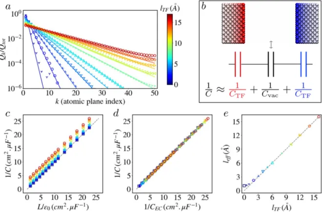
FIG. 2. Empty Thomas–Fermi capacitor. All results correspond to a (100) gold-like electrode structure with n = 50 atomic planes and L = 300 Å between the electrodes where
not stated otherwise. Charges are computed by applying a voltageΔΨ = 1 V between the electrodes for different Thomas–Fermi lengths lTFranging from 0.0 Å to 16.0 Å,
which are represented both by different symbols and by different colors indicated by the color bar. (a) Total charge per plane on the positive electrode as a function of the position from the surface (k is the index of the atomic plane), normalized by the total electrode charge Qtot(only values for lTF>0.5 Å are shown). The symbols are simulated values for different Thomas–Fermi lengths lTF, and the lines are the prediction of Eq.(7). (b) Snapshot of the simulated system and its equivalent circuit representation
corresponding to the capacitance obtained with the continuum theory (see the text). (c) Computed reciprocal capacitance as a function of the analytical predictions for perfect metals usingLvac= L and (d) for Thomas–Fermi metals using Eq.(8)withLvac= L − a for varying electrode spacing L (between 10 Å and 200 Å). (e) Effective length leff,
defined in Eq.(9), as a function of lTF.
J. Chem. Phys. 153, 174704 (2020); doi: 10.1063/5.0028232 153, 174704-3
III. EMPTY CAPACITOR
As a first validation of our implementation, we study a model system composed of two planar (100) gold electrodes sep-arated by a distance L and held at a constant potential differ-ence ΔΨ = 1 V. Each electrode consists of n atomic planes with an inter-spacing a in the z direction. We compare the simulated results against analytical predictions of the corresponding contin-uum model where the Poisson equation for the one-dimensional potential Ψ(z) reads Ψ′′
(z) = l−2TFΨ(z) inside each electrode and Ψ′′
(z) = 0 between them. The total capacitance of the system is given byC = Qtot/ΔΨ.
Assuming that the width of the material is large compared to the Thomas–Fermi length, the in-plane chargeQkatz = ka (k ∈ [1, n]) can be expressed as
Qk Qtot =e
−(k−1)a/lTF
[1 −e−a/lTF]. (7)
Figure 2(a)shows a very good agreement between Eq.(7)and the simulation for largelTF values. Small deviations are observed for largez due to the finite number of planes and for lTFvalues smaller than characteristic atomic lengths where the continuum prediction is not expected to hold. The above exponentially decaying charge distribution inside the metal, due to the screening over the Thomas– Fermi lengthlTF, results according to the continuous model in a capacitance per unit area,
1 CEC = 1 Cvac + 2 CTF = Lvac ϵ0 +2lTF ϵ0 , (8)
withCvac= ϵ0/Lvacbeing the theoretical capacitance per unit area for perfect metallic electrodes (lTF = 0.0 Å) separated by a vac-uum slab of width Lvac and CTF = ϵ0/lTF being that for a sin-gle Thomas–Fermi electrode. This result can be simply understood in terms of the equivalent circuit (hence the subscriptCEC) illus-trated inFig. 2(b), with three capacitors in series (see Sec. S1 of the
supplementary materialfor a discussion of the continuum descrip-tions and equivalent circuit models). As shown in Fig. 2(c), the simulation results are consistent with the prediction of a linear rela-tion between 1/C and L/ϵ0, whereL is the distance between the first
atomic planes on each electrode, with a constant shift that increases withlTF.
However, the width of the vacuum slab between the elec-trodes is not exactly the distance between the first atomic planes. Indeed, each atomic site is surrounded by electrons, and the bound-ary between the free electron gas inside the electrode and the vac-uum25(the so-called “Jellium edge”26) is rather shifted half of the inter-plane distance away from the electrode. Since this feature is present on both electrodes, the actual vacuum slab width is more consistent with Lvac = L − a. Figure 2(d)shows that using this prescription, Eq.(8)provides a very good description of the sim-ulated capacitanceC over a wide range of distances between the electrodes and Thomas–Fermi lengths, which confirms the consis-tency of the present classical model to represent the charge distri-bution within the metal. The decay length of the charge inside the electrode coincides withlTF within 1% for all valueslTF≳a. The slight deviations from the predictions of the continuous theory can be analyzed by introducing an effective lengthlefffrom the measured capacitance as 1 C= L − a ϵ0 +2leff ϵ0 . (9)
The results obtained for variouslTFat fixedL, illustrated inFig. 2(e), indicate that this effective length deviates from the Thomas–Fermi length only when the latter becomes comparable to the atomic details of the electrodes (interplane and interatomic distances, width of the Gaussian distributions). An additional test was performed by adding a single charge at various distances between the electrodes and comparing the energy of the system to an approximate analyt-ical expression.12The results, which are provided in Sec. S2 of the
supplementary material, also show a good agreement over a broad range oflTFvalues.
IV. IMPACT OF THE THOMAS–FERMI LENGTH
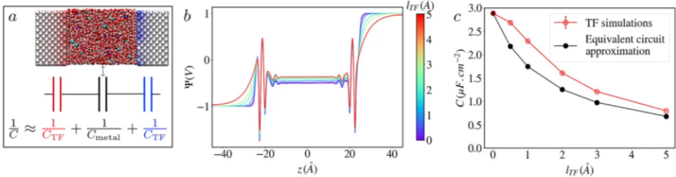
ON THE ELECTROCHEMICAL INTERFACE PROPERTIES In order to understand the impact of screening inside the metal on the properties of electrode/electrolyte interfaces, we study
FIG. 3. The capacitance decreases significantly with the Thomas–Fermi length. (a) Snapshot of the simulated system and its equivalent circuit representation, where Cmetal
stands for the capacitance computed for the perfect metal simulation. (b) Poisson potential across the simulation cell for a system made of two (100) gold-like electrodes in contact with a NaCl aqueous solution. The applied voltage is 2 V and different lTFvalues ranging from 0.0 Å to 5.0 Å are represented by different colors indicated in the color
bar. The screening of the potential inside the electrodes increases markedly with lTF. (c) Variation of the capacitance with lTF. The results from the simulations are compared
The Journal
of Chemical Physics
ARTICLE scitation.org/journal/jcpa system consisting of two (100) gold-like electrodes in contact with an aqueous solution of NaCl (with concentration 1 mol l−1), illus-trated inFig. 3(a). The TF lengthlTFwas systematically varied from 0.0 Å to 5.0 Å in order to switch from a perfect metal to typical semi-metallic conditions (estimations yield typical values of 0.5 Å for platinum, 1.5 Å for doped silicon, and 3.4 Å for graphite11). Sim-ulations were performed for voltages ΔΨ = 0 V, 1 V, and 2 V between the two electrodes.
As a first illustration of the impact of screening on the electro-chemical interface, we compute the Poisson potential across the cell.
The results for an applied potential of 2 V are displayed onFig. 3(b). We observe a very different pattern inside the electrode depend-ing onlTF: for the perfect metal, the applied potential is reached at positions corresponding to the first atomic plane, while for the TF model, we clearly see the desired effect of field penetration with an exponential decay inside the electrode. Note also that at the largest applied voltage, the average atomic charge ranges between 0.02e for lTF= 0 Å and 0.003e for lTF= 5 Å (with corresponding standard devi-ations of 0.01e and 0.001e), which validates a posteriori the hypoth-esis on the number of free charge carriers being smaller than the
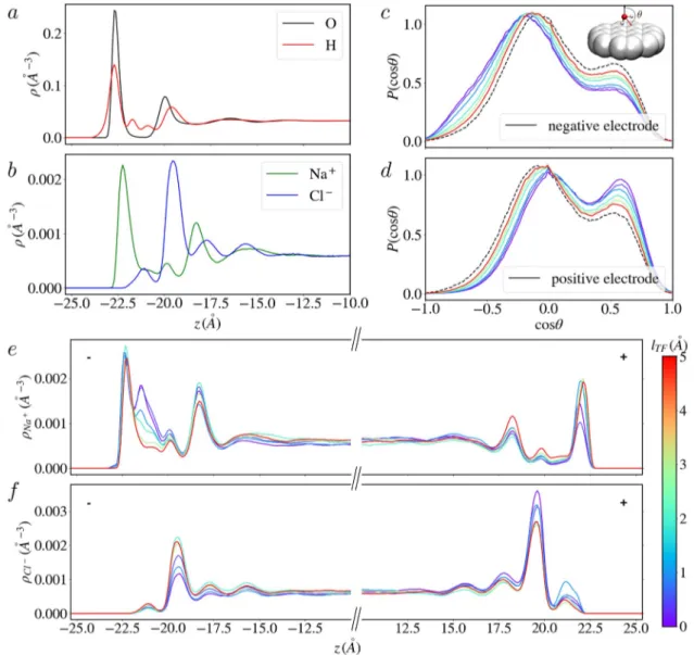
FIG. 4. The structure of the electrochemical interface depends on the Thomas–Fermi length at finite voltages. [(a) and (b)] Atomic density profiles for the O, H, Na+, and Cl−
atoms near the electrode at null potential for lTF= 0.0 Å (the profiles are the same for the other lTFvalues, as shown in Fig. S3 of thesupplementary material). Note that in the
case of H atoms, the profile is divided by two to facilitate the comparison with O atoms. [(c) and (d)] Distribution of the orientation of adsorbed water molecules with respect to the vector normal to the electrode surfaces for an applied potential of 2 V for the whole range of simulated lTFindicated by the color bar; the distribution for 0 V and lTF
= 0.0 Å is also reported (black dashed lines) as a reference. [(e) and (f)] Atomic density profiles for the Na+and Cl−ions for an applied potential of 2 V for the whole range of
simulated lTFindicated by the color bar. The negative (positive) electrode is located at negative (positive) z.
J. Chem. Phys. 153, 174704 (2020); doi: 10.1063/5.0028232 153, 174704-5
number of electrons made in the derivation of the TF electrode model.
Figure 3(c)shows that the integral capacitance decreases sig-nificantly withlTF(note that it remains constant between 1 V and 2 V and that the decrease is of similar magnitude for the individ-ual capacitance of the positive and negative electrodes; see Fig. S2 of thesupplementary material). The effect is already non-negligible forlTF= 0.5 Å (which is representative of many real metals) since the capacitance is 7% smaller than the one of the perfect metal; it is even more pronounced in the semi-metallic régime. This can be understood by noting that the TF length varies as the inverse square-root of the number of available states at the Fermi level. In a perfect metal, the number of accessible states is infinite so that the only resistance to charging arises from the Coulombic energy. In contrast, the TF model results in an additional energy penalty for increasing the surface charge, described by the quadratic term in Eq.(6).
As for the empty capacitor, it is possible to estimate the capac-itance from the value for the perfect metalCmetalusing the equiva-lent circuit depicted onFig. 3(a)(see Sec. S1 of thesupplementary material). This approach, used by Gerischer to interpret experimen-tal data,27 has been applied in many simulation works where the additional term due to the screening was computed using DFT and therefore called “quantum capacitance,” while the perfect metal capacitance was computed using either a mean-field the-ory10or molecular dynamics.28Nevertheless, it neglects the interplay between the electronic structure of the electrode and the ionic struc-ture of the adsorbed electrolyte. This coupling is self-consistently taken into account in our model, which therefore provides a per-fect framework to test this approximation. As shown inFig. 3(c), the equivalent circuit approximation underestimates rather significantly the real capacitance (by 20%–30%).
At null voltage, the average structure of the liquid does not vary significantly withlTF(see Fig. S3 of thesupplementary material). As shown inFigs. 4(a)and4(b), it is characterized by several adsorption layers, mainly consisting of water molecules. By computing the dis-tribution of the angle θ between the vector normal to the surface and the water dipole [see the black dashed curve inFigs. 4(c)and4(d)] or the O–H bonds (see Fig. S4 of thesupplementary material) for molecules in the first adsorbed layer, we observe that they mostly lie in a plane parallel to the surface or with one H atom pointing away from the surface. A small population is oriented toward the surface, which results in a small shoulder on atomic density profiles of the H atoms.
The ions have different adsorption profiles: the Na+density is characterized by a large peak located close to one of the O atoms so that they can be considered to belong to the first layer, while the Cl− ions are located further away from the electrode surface. Their pro-file displays a small pre-peak in the region where the water density is very low and a peak with a larger intensity located in the sec-ond hydration layer. Once a potential is applied, the liquid mainly responds to the two electrodes through (i) a stronger orientation of the water molecules toward/away from the negative/positive elec-trode, as shown inFigs. 4(c)and 4(d)and Figs. S4 and S5 of the
supplementary material, and (ii) the appearance of a new adsorption peak for the Na+ions near the negative electrode [Fig. 4(e)] and an increase in the pre-peak intensity in the Cl−density profiles on the positive electrode side [Fig. 4(f)]. In all cases, the modifications in
FIG. 5. The relaxation of the electrode charge indicates a faster dynamics of the
interfacial electrolyte near screened metals. Normalized auto-correlation function of the total charge at null potential for varying lTFvalues ranging from 0.0 Å to
5.0 Å indicated by the color bar.
the structure depend strongly onlTF. This shows that depending on the type of material, we can expect all the electrochemical double-layer properties to change markedly with the nature of the chosen electrode.
Dynamical properties are particularly important for electro-chemical applications. They control the power delivered by an energy storage device. The equilibrium fluctuations of the electrode charge at 0 V, which reflect the linear response to a small applied voltage, are shown inFig. 5for variouslTF. An increased screen-ing yields faster dynamics for the relaxation of the electrochemical double-layer. Such a difference was somewhat unexpected given that the systems at null potential have, on average, the same structural features, but it can be qualitatively understood as the result of weaker interactions with the more diffuse charges induced within the elec-trode. This means that the dynamics do not only depend on the nature of the electrolyte but also depend on the electronic structure of the electrode material.
V. CONCLUSION
Understanding the electrode/electrolyte interface is a prerequi-site not only for the design of more efficient energy storage devices29 but also for understanding wetting phenomena involved in lubri-cation or heterogeneous catalysis.30Although in the past decades, molecular simulations have provided much insight into the struc-ture of the electrochemical double-layer, they still fail at predicting quantitatively many experimental quantities, such as the variation of the differential capacitance with the applied voltage.31This is par-ticularly true in the case of carbon materials due to their complex electronic structure properties that deviate largely from the ones of typical metals. Many intriguing experimental observations, such as the capillary freezing of ionic liquids confined between metal-lic surfaces11and the emergence of longer-than-expected
electro-static screening lengths in concentrated electrolytes,32,33remain to be explained quantitatively. The Thomas–Fermi model, by allowing to tune the metallicity of the electrode using a single parameter (also without introducing additional computational costs), should lead to
The Journal
of Chemical Physics
ARTICLE scitation.org/journal/jcpa more accurate understanding of the interfacial properties of such electrodes using molecular simulations. The extension of this work to complex materials such as nanoporous carbons will require addi-tional efforts in order to take into account the effect of the local environment of each atom on its electronic response. In that case, it might be relevant to sacrifice some of the simplicity of the TF model by including atom-specific or even bond-specific terms in the energy, following the split charge equilibration approach.34,35In this
context, the present work suggests that it could be possible to deter-mine the associated parameters from a simplified representation of the underlying electronic density.
SUPPLEMENTARY MATERIAL
See theSupplementary materialfor a discussion on the con-tinuum description and equivalent circuit models, additional tests for a single charge between two electrodes, additional results on the differential capacitances of the two electrodes and their variation with the Thomas–Fermi length, and additional structural charac-terizations of the aqueous NaCl electrolyte put in contact with the gold-like electrodes at 0 V and 2 V.
AUTHORS’ CONTRIBUTIONS
L.S. and T.D. contributed equally to this work.
ACKNOWLEDGMENTS
The authors thank M. Sprik, P. A. Madden, L. Bocquet, and B. Coasne for useful discussions. This project received fund-ing from the European Research Council under the European Union’s Horizon 2020 research and innovation program (Grant Agreement No. 771294). This work was supported by the French National Research Agency [Labex STORE-EX (Grant No. ANR-10-LABX-0076), project SELFIE (Grant No. ANR-17-ERC2-0028), and project NEPTUNE (Grant No. ANR-17-CE09-0046-02)]. The authors acknowledge HPC resources granted by GENCI (resources of CINES; Grant No. A0070911054).
APPENDIX: SIMULATION DETAILS
The TF electrode model was implemented in the molecu-lar dynamics code MetalWalls.36 All simulations were run using a matrix inversion method5 to enforce both the constant
poten-tial and the electroneutrality constraints on the charges. Electrode atoms have a Gaussian charge distribution of width η−1= 0.56 Å centered on zero, and the Thomas–Fermi lengthlTFranges from 0.0 Å to 16.0 Å for the empty capacitor and from 0.0 Å to 5.0 Å in the presence of an aqueous NaCl electrolyte. Two-dimensional boundary conditions were used with no periodicity in thez direc-tion using an accurate 2D Ewald summadirec-tion method to compute electrostatic interactions. A cutoff of 17.0 Å was used for both the short range part of the Coulomb interactions and the intermolecular interactions. For the latter, we used the truncated shifted Lennard-Jones potential. The box length in both thex and y directions was Lx=Ly= 36.630 Å with 162 atoms per atomic plane. The structure
is face-centered cubic with a lattice parameter of 4.07 Å and a sepa-ration between planesa = 2.035 Å in the (100) direction (the atomic densityd is 0.59 ⋅ 1029 m−3). The empty capacitors have 50 planes per electrode, whereas the electrochemical cells have 10 (leading to a total of 1620 atoms per electrode). In the latter case, the electrolyte is composed of 2160 water molecules, modeled using the SPC/E force field,37and 39 NaCl ion pairs. The Lennard-Jones parameters for Na+and Cl−were taken from Ref.38and the ones for the electrode atoms from Ref.39; the Lorentz–Berthelot mixing rules were used. The simulation boxes were equilibrated at a constant atmospheric pressure for 500 ps by applying a constant pressure force to the elec-trodes withlTF= 0.0 Å, and then, the electrode separation was fixed to the equilibrium value (for which the density in the middle of the liquid slab is equal to its bulk value)L = 56.8 Å. The simulations were run at 298 K with a time step of 1 fs. Each system was run for at least 8 ns.
DATA AVAILABILITY
The code used for the simulations and the data that support the findings of this study are openly available in the repository
https://gitlab.com/ampere2.
REFERENCES
1J. I. Siepmann and M. Sprik, “Influence of surface-topology and electrostatic potential on water electrode systems,”J. Chem. Phys.102, 511–524 (1995). 2
C. Merlet, B. Rotenberg, P. A. Madden, P.-L. Taberna, P. Simon, Y. Gogotsi, and M. Salanne, “On the molecular origin of supercapacitance in nanoporous carbon electrodes,”Nat. Mater.11, 306–310 (2012).
3
S. Bi, H. Banda, M. Chen, L. Niu, M. Chen, T. Wu, J. Wang, R. Wang, J. Feng, T. Chen, M. Dinc˘a, A. A. Kornyshev, and G. Feng, “Molecular understanding of charge storage and charging dynamics in supercapacitors with MOF electrodes and ionic liquid electrolytes,”Nat. Mater.19, 552–558 (2020).
4D. T. Limmer, A. P. Willard, P. Madden, and D. Chandler, “Hydration of metal surfaces can be dynamically heterogeneous and hydrophobic,”Proc. Natl. Acad. Sci. U. S. A.110, 4200–4205 (2013).
5L. Scalfi, D. T. Limmer, A. Coretti, S. Bonella, P. A. Madden, M. Salanne, and B. Rotenberg, “Charge fluctuations from molecular simulations in the constant-potential ensemble,”Phys. Chem. Chem. Phys.22, 10480–10489 (2020). 6L. Scalfi, M. Salanne, and B. Rotenberg, “Molecular simulation of electrode-solution interfaces,”arXiv:2008.11967(2020).
7
A. A. Kornyshev and M. A. Vorotyntsev, “Analytic expression for the potential energy of a test charge bounded by solid state plasma,”J. Phys. C: Solid State Phys. 11, L691–L694 (1978).
8
A. A. Kornyshev, W. Schmickler, and M. A. Vorotyntsev, “Nonlocal electrostatic approach to the problem of a double layer at a metal-electrolyte interface,”Phys. Rev. B25, 5244–5256 (1982).
9
N. B. Luque and W. Schmickler, “The electric double layer on graphite,” Elec-trochim. Acta71, 82–85 (2012).
10A. A. Kornyshev, N. B. Luque, and W. Schmickler, “Differential capacitance of ionic liquid interface with graphite: The story of two double layers,”J. Solid State Electrochem.18, 1345–1349 (2014).
11J. Comtet, A. Niguès, V. Kaiser, B. Coasne, L. Bocquet, and A. Siria, “Nanoscale capillary freezing of ionic liquids confined between metallic interfaces and the role of electronic screening,”Nat. Mater.16, 634–639 (2017).
12V. Kaiser, J. Comtet, A. Niguès, A. Siria, B. Coasne, and L. Bocquet, “Electro-static interactions between ions near Thomas-Fermi substrates and the surface energy of ionic crystal at imperfect metals,”Faraday Discuss.199, 129–158 (2017). 13L. H. Thomas, “The calculation of atomic fields,”Math. Proc. Cambridge Philos. Soc.23, 542–548 (1927).
J. Chem. Phys. 153, 174704 (2020); doi: 10.1063/5.0028232 153, 174704-7
14
E. Fermi, “Un metodo statistico per la determinazione di alcune proprietà dell’atomo,” Rend. Accad. Naz. Lincei 6, 602–607 (1927).
15
S. K. Reed, O. J. Lanning, and P. A. Madden, “Electrochemical interface between an ionic liquid and a model metallic electrode,”J. Chem. Phys.126, 084704 (2007).
16E. Paek, A. J. Pak, and G. S. Hwang, “On the influence of polarization effects in predicting the interfacial structure and capacitance of graphene-like electrodes in ionic liquids,”J. Chem. Phys.142, 024701 (2015).
17
R. F. Nalewajski, “Electrostatic effects in interactions between hard (soft) acids and bases,”J. Am. Chem. Soc.106, 944–945 (1984).
18W. J. Mortier, S. K. Ghosh, and S. Shankar, “Electronegativity-equalization method for the calculation of atomic charges in molecules,”J. Am. Chem. Soc. 108, 4315–4320 (1986).
19A. K. Rappe and W. A. Goddard III, “Charge equilibration for molecular dynamics simulations,”J. Phys. Chem.95, 3358–3363 (1991).
20
N. Onofrio, D. Guzman, and A. Strachan, “Atomic origin of ultrafast resis-tance switching in nanoscale electrometallization cells,”Nat. Mater.14, 440–446 (2015).
21
M. Buraschi, S. Sansotta, and D. Zahn, “Polarization effects in dynamic inter-faces of platinum electrodes and ionic liquid phases: A molecular dynamics study,” J. Phys. Chem. C124, 2002–2007 (2020).
22
D. M. York and W. Yang, “A chemical potential equalization method for molecular simulations,”J. Chem. Phys.104, 159–172 (1996).
23H. Nakano and H. Sato, “A chemical potential equalization approach to constant potential polarizable electrodes for electrochemical-cell simulations,” J. Chem. Phys.151, 164123 (2019).
24L. Pastewka, T. T. Järvi, L. Mayrhofer, and M. Moseler, “Charge-transfer model for carbonaceous electrodes in polar environments,”Phys. Rev. B83, 165418 (2011).
25N. D. Lang and W. Kohn, “Theory of metal surfaces: Induced surface charge and image potential,”Phys. Rev. B7, 3541–3550 (1973).
26
N. V. Smith, C. T. Chen, and M. Weinert, “Distance of the image plane from metal surfaces,”Phys. Rev. B40, 7565–7573 (1989).
27
H. Gerischer, “An interpretation of the double layer capacity of graphite elec-trodes in relation to the density of states at the Fermi level,”J. Phys. Chem.89, 4249–4251 (1985).
28
A. J. Pak, E. Paek, and G. S. Hwang, “Relative contributions of quantum and double layer capacitance toward the supercapacitor performance of carbon nanotubes in an ionic liquid,”Phys. Chem. Chem. Phys.15, 19741–19747 (2013). 29
M. Salanne, B. Rotenberg, K. Naoi, K. Kaneko, P.-L. Taberna, C. P. Grey, B. Dunn, and P. Simon, “Efficient storage mechanisms for building better super-capacitors,”Nat. Energy1, 16070 (2016).
30
J. Carrasco, A. Hodgson, and A. Michaelides, “A molecular perspective of water at metal interfaces,”Nat. Mater.11, 667–674 (2012).
31M. V. Fedorov and A. A. Kornyshev, “Ionic liquids at electrified interfaces,” Chem. Rev.114, 2978–3036 (2014).
32
M. A. Gebbie, M. Valtiner, X. Banquy, E. T. Fox, W. A. Henderson, and J. N. Israelachvili, “Ionic liquids behave as dilute electrolyte solutions,”Proc. Natl. Acad. Sci. U. S. A.110, 9674–9679 (2013).
33
A. M. Smith, A. A. Lee, and S. Perkin, “The electrostatic screening length in concentrated electrolytes increases with concentration,”J. Phys. Chem. Lett.7, 2157–2163 (2016).
34
R. A. Nistor, J. G. Polihronov, and M. H. Müser, “A generalization of the charge equilibration method for nonmetallic materials,” J. Chem. Phys.125, 094108 (2006).
35
R. A. Nistor and M. H. Müser, “Dielectric properties of solids in the regular and split-charge equilibration formalisms,”Phys. Rev. B79, 104303 (2009). 36A. Marin-Laflèche, M. Haefele, L. Scalfi, A. Coretti, T. Dufils, G. Jeanmairet, S. Reed, A. Serva, R. Berthin, C. Bacon, S. Bonella, B. Rotenberg, P. A. Madden, and M. Salanne, “Metalwalls: A classical molecular dynamics software dedicated to the simulation of electrochemical systems,”J. Open Source Software5, 2373 (2020).
37H. J. C. Berendsen, J. R. Grigera, and T. P. Straatsma, “The missing term in effective pair potentials,”J. Phys. Chem.91, 6269–6271 (1987).
38
L. X. Dang,J. Am. Chem. Soc.117, 6954 (1995). 39