HAL Id: tel-01958678
https://pastel.archives-ouvertes.fr/tel-01958678
Submitted on 18 Dec 2018HAL is a multi-disciplinary open access archive for the deposit and dissemination of sci-entific research documents, whether they are pub-lished or not. The documents may come from teaching and research institutions in France or abroad, or from public or private research centers.
L’archive ouverte pluridisciplinaire HAL, est destinée au dépôt et à la diffusion de documents scientifiques de niveau recherche, publiés ou non, émanant des établissements d’enseignement et de recherche français ou étrangers, des laboratoires publics ou privés.
Description des processus physiques pilotant le cycle de
vie de brouillards radiatifs et des transitions
brouillard–stratus basé de modèles conceptuels
Eivind Wærsted
To cite this version:
Eivind Wærsted. Description des processus physiques pilotant le cycle de vie de brouillards radiatifs et des transitions brouillard–stratus basé de modèles conceptuels. Meteorology. Université Paris-Saclay, 2018. English. �NNT : 2018SACLX053�. �tel-01958678�
NNT
:2018SA
CLX053
Description of physical processes driving
the life cycle of radiation fog and
fog–stratus transitions based on
conceptual models
Th`ese de doctorat de l’Universit´e Paris-Saclaypr´epar´ee `a ´Ecole Polytechnique Ecole doctorale n◦579 Sciences m´ecaniques et ´energ´etiques, mat´eriaux et
g´eosciences (SMEMAG)
Sp´ecialit´e de doctorat : M´et´eorologie, oc´eanographie, physique de l’environnement
Th`ese pr´esent´ee et soutenue `a Palaiseau, le 12.10.2018, par
E
IVINDW
ÆRSTEDComposition du Jury :
Philippe Drobinski
Directeur de recherche CNRS, LMD (UMR-8539) Pr´esident Marie Lothon
Charg´ee de recherche CNRS, LA (UMR-5560) Rapporteur Pierre Gentine
Professor Columbia University, EEE Rapporteur Gert-Jan Steeneveld
Associate Professor, Wageningen University, MAQ Examinateur Christine Lac
Ing´enieur ICPEF M´et´eo-France, CNRM (UMR-3589) Examinatrice Marjolaine Chiriaco
Maˆıtre de conf´erences UVSQ, LATMOS Examinatrice Martial Haeffelin
Ing´enieur de recherche CNRS, IPSL (FR-636) Directeur de th`ese Jean-Charles Dupont
Physicien adjoint UVSQ, IPSL (FR-636) Co-encadrant de th`ese Marie Vicomte
Ing´enieur Direction G´en´erale de l’Armement Invit´ee Damien Vignelles
Acknowledgements
This PhD thesis has been a great experience for me, both professionally and personally. For the first time of my life, I have lived abroad for a longer time period, and I got the chance to live in a big city and be in touch with a large and diverse research environment of atmospheric sciences. One motivation for choosing this particular thesis was the possibility to work closer to the actual observations of the atmosphere and clouds. Being part of the SIRTA team, with occasional field work at the observatory, and the direct use of observational data, has been just the enriching experience I had hoped for. I would like to thank the financial organisms of my thesis, the Direction Générale de l’Armement, and the company Meteomodem, for granting me the scholarship that allowed me to study fog for the past 3 years.
I give a great thanks to my main supervisor, Martial Haeffelin, who has put a lot of time and energy into our weekly discussions of my work. He has always been available to answer my questions or help me find a new direction when everything seemed to be stuck. There has always been a vast amount of alternative angles of attack and pists to pursue, not least due to the very large and multi-instrumental fog dataset that has been at my disposal, and the clarifying discussions with Martial have been essential for keeping up the progress. I would also like to thank my co-supervisor Jean-Charles Dupont, who has followed my work closely as well and answered my questions to help me interpret my results. His practical knowledge about the SIRTA instrument park has been very important for being able to understand and correctly apply the observational data. The whole SIRTA team has also been helpful with processing the data we had particular need of and the deployment of specific instruments in the fog season. The comprehensive observations at SIRTA are supported through the ACTRIS-2 project, which is funded by the European Union’s Horizon 2020 research and innovation programme under grant agreement No 654109. The BASTA cloud radar, which is one of the main tools used in my thesis, is maintained and developed by Julien Delanoë of LATMOS, and his help with understanding the radar has been very important for my work. Felipe Toledo also helped me understanding better the functioning of radars in general. I would also like to acknowledge those who participated in the early-morning balloon flights with the droplet-counting instrument LOAC, and Jean-Baptiste Renard for helping us understand and use the LOAC.
In spite of the large observational dataset, modelling has been an essential part of my thesis. I have needed the models to understand the mechanisms we observe and their sensitivities, and to estimate the variables that we do not directly observe, especially the processes at fog top. The application of the radiative transfer model ARTDECO allowed us to study the very important fog-top radiative fluxes. I thank Philippe Dubuisson from LOA at the University of Lille as well as Victor Winiarek, for their assistance in setting up the model runs with ARTDECO. Thanks to the ICARE Data and Services Center for providing access to the ARTDECO code and the associated datasets.
this PhD thesis, using large-eddy simulations (LES). This was possible thanks to Gert-Jan Steeneveld, who welcomed me to a 3 months stay at his institute in Wageningen in the Netherlands, and to the WIMEK, who financed this stay. Gert-Jan has always been very positive and interested in our work with the large-eddy model and patient to explain the technical aspect to someone who had never worked with LES before. I learned a lot during the stay in the Netherlands, not least because of the new processes I had to understand, especially the surface energy balance and entrainment at the top of well-mixed boundary layers. The expertise of the Dutch researchers on atmosphere–vegetation interactions and boundary-layer turbulence was very valuable for me. In addition to Gert-Jan, I would especially like to thank Arnold Moene, Stephan de Roode, Chiel van Heerwarden, Jordi Vila, Huug Ouwersloot, Xabier Pedruzo Bagazgoitia and Fred Bosveld for important discussions on how best to understand the fog interactions with the surface and the layer above its top, and how to set up the LES in a good way. The simulations were also made possible thanks to the SURFsara supercomputer facilities with the financial support of the Netherlands Organisation for Scientific Research (NWO) Physical Science Division (project number SH-312-15). The ACTRIS Trans-National Access program funded a visit of Gert-Jan to Paris some time after the 3-months stay, which helped us continue our collaboration.
We also applied data from the reanalysis ERA5 in the fog analysis. These were provided through ECMWF, COPERNICUS Climate Change Service data, available from the ESPRI/IPSL data center. There are also many colleges at LMD other than my supervisors who helped me understand and develop the concepts of my thesis. In particular, I had fruitful discussions with Jordi Badosa, Simone Kotthaus, Juan Antonio Bravo-Aranda, Thibault Vaillant de Guélis, Felipe Toledo, Olivier Atlan and Jan Polcher. I also want to thank Gaëlle Clain, Pauline Martinet, Maud Pastel and Julien Delanoë for participating in my monitoring committee, and Pierre Gentine and Marie Lothon for accepting to be reviewers for my thesis. Thanks also to all the other members of my defence committee for evaluating my PhD project: Christine Lac, Marjolaine Chiriaco, Philippe Drobinski, Gert-Jan Steeneveld, Damien Vignelles and Marie Vicomte.
A research project like mine requires a lot of work dedicated to writing, debugging and under-standing programming code, as well as logging into various computers. I would here like to give a special thanks to Marc-Antoine Drouin for his help with computer technicalities, which he has always been very willing to give at almost any time. Julien Lenseigne has also helped me out with technical problems of a wide range, such as helping me make the printer print my thesis correctly, and providing me with a keyboard when the built-in one in my Macbook was broken.
Coming to work in France is specifically challenging due to the formalities involved, even when I did not need a visa or work permit. Thanks to the administration staff (Isabelle Ricordel, France-Lise Robin, Gaëlle Bruant, Grégory Boucher), my supervisor Martial, and Imma Bastida for helping me out with various forms. Thanks to Xavier Quidelleur and Kim Ho of the Smemag doctoral school for the good communication regarding my yearly re-registrations and validation of courses. Thanks also to Emmanuel Fullenwarth and Aurélien Arnoux for the very clear instructions and good communication regarding the intricate formalities required for the thesis defence and legal deposits of my dissertation. On the wider aspect of living in France, I would also like to thank the organisation Science Accueil for preparing my stay in France by enabling me to open a bank account before I arrived and giving me explanations on which insurances I needed to get. I also very much appreciate being allowed to live at the excellent student house Maison de Norvège in Cité Universitaire for my whole stay. All of
the staff there has been very kind and helpful, and I have enjoyed staying with my fellow residents – thank you all first-floorers! Thanks also to my very nice fellow residents in the apartment where I lived during my stay in Wageningen. I am also thankful for the very inclusive Trinity International Church of Paris and the friendly young people I got to know there.
I very much appreciated the social activities among the PhD students and Post-docs at LMD, including football, board games and evenings out in Paris. Bastien, Nicolas, Oliver, Felipe, Aurore, Artemis, Stavros, Thibault, Adrien, Rodrigo, Xudong, Ariel, Sara, Fuxing, Erik, Trung, Alexis, I am going to miss you all.
A very special thanks goes to my girlfriend Beate, who has been patiently waiting for me back in Norway all this time. Thanks for our pleasant short holidays together every 2 months or so, which have been very nice breaks from life as a PhD student. Thanks also to Beate’s family for welcoming me into their homes during the holidays and bringing me on their Europe road trip.
Finally, thanks to my own family for the regular contact during my stay in France and their interest in my work. Thanks in particular to my father Morten who is always available when I need encouragement and advice. I am also thankful for the care and concern of my grandmother Sigrun. My uncle Kristian and aunt Liv have always been very supportive, especially since the early death of my mother. I am also, as I always have been, very happy to have my large and fast growing Danish family, who I go to see every year at Christmas.
Abstract
Fog causes hazards to human activities due to the reduction of visibility, especially through the risk of traffic accidents. The fog life cycle is driven by radiative, dynamical, and microphysical processes which interact with each other in complex manners that are not yet fully understood. Improving our understanding of these processes and our ability to forecast fog formation and dissipation is therefore an objective for research. This thesis analyses the life cycle of continental fog events occurring in the Paris area, using several ground-based remote sensing instruments deployed at the SIRTA atmospheric observatory. We focus on understanding the dissipation after sunrise and the local processes involved. Over a 4-year period, more than 100 fog events are documented by observing cloud base height (CBH) (with ceilometer), cloud top height (CTH) and clouds appearing above the fog (with cloud radar), and the liquid water path (LWP) (with microwave radiometer (MWR)). When combined with the cloud radar, the MWR also provides estimates of the integrated water vapour (IWV) above the fog and the thermal stratification of the layer above fog top.
Most fog events dissipate by lifting of the CBH without a complete evaporation of the cloud, and sometimes even without a reduction in LWP. This is because an increase in the CTH can also trigger fog dissipation. In fact, by applying the model of Cermak and Bendix (2011), we find that the LWP and CTH are the principal parameters which determine the CBH and therefore fog dissipation. For each CTH, there is a critical fog LWP which must be exceeded if the fog should stay at the surface. This critical LWP increases more than linearly with CTH, and for a fog temperature of 5 ◦C it is estimated to 6 g m−2 for a CTH of 100 m, 29 g m−2 for 200 m, and 131 g m−2 for 400 m. In order to better understand fog dissipation, we therefore focus on the impacts of the physical processes on LWP and CTH. Using a radiative transfer code and large-eddy simulations (LES), we quantify the impacts on the two parameters by the processes of long-wave (LW) radiation, short-wave (SW) radiation, surface turbulent heat fluxes, fog-top entrainment, large-scale subsidence and droplet deposition, and we study the parameters which can cause important variability in these impacts. We also develop a conceptual framework based on a well-mixed assumption to be able to calculate the impacts that estimated heat and moisture fluxes have on the fog LWP.
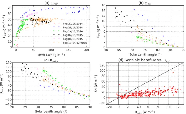
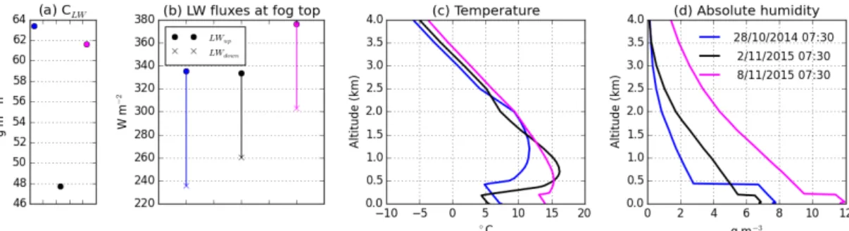
Radiative processes are studied using the comprehensive radiative transfer code ARTDECO. The LW radiative cooling at fog top can produce 40–70 g m−2 h−1 of LWP when the fog is opaque (LWP >≈ 30 g m−2) and there are no clouds above. This cooling is the main process of LWP production
and can renew the fog LWP in 0.5–2 h. Its variability is mainly explained by the fog temperature and the humidity profile above the fog. Clouds above the fog will strongly reduce this production, especially low clouds: a cloud with optical depth 4 can reduce it by 30 (100) % when located at 10 (2) km. When the fog is semi-transparent to LW radiation, corresponding to LWP <≈ 30 g m−2, which is the case for nearly half the fog dataset, the LWP production increases strongly with LWP. Loss of LWP by absorption of solar radiation by the fog is 5–15 g m−2 h−1 around midday in winter,
increasing with cloud thickness, but it can be enhanced by 100 % in case of important amounts of absorbing aerosols (case tested: a population of urban aerosols with dry aerosol optical depth of 0.15 and single scattering albedo of 0.82).
Heating of the fog due to solar radiation absorbed at the surface, through turbulent heat fluxes, is found to be the dominating process of LWP loss after sunrise and can reach 20–30 g m−2 h−1 (according to LES), but its magnitude is sensitive to the Bowen ratio. However, observations of the turbulent heat fluxes during fog are not precise enough to determine the Bowen ratio. Its importance for fog LWP budget shows that improved understanding and measurements of the Bowen ratio during fog should be a priority. Through its impact on the Bowen ratio, the liquid water on the surface can be important for fog persistence in the morning; in our LES study, fog dissipates 85 min later in a run with 50 % of the surface covered by liquid water, compared to a run with no surface water.
Observations by radiosondes reveal the variability of the thermal stratification and humidity of the layer above the fog top. Using the LES, we find a strong sensitivity of the vertical development of the fog top to this observed variability in stratification. By enhancing entrainment, a weak stratification at fog top can lead to earlier fog dissipation by (1) more depletion of LWP by entraining unsaturated air, especially if the air is dry, and (2) increase in CTH. Fog dissipation is 90 min earlier in an LES sensitivity test using a weak stratification relative to the baseline run with a strong stratification. The variability of this stratification in the radiosondes can be observed reasonably well with the MWR temperature profile, which allows continuous time series of this parameter. The variability in the humidity above fog top also has an important impact on the dissipation time: in our LES sensitivity test with dry overlying air, the fog dissipates 70 min earlier than in the baseline run with air above close to saturation. The drier air causes faster depletion of fog LWP, allowing the fog to lift earlier. However, the effect of humidity above is sensitive to the details of the humidity profile, since a dry atmosphere also increases LW radiative cooling.
In order to investigate the results presented above for a larger number of fog events, we develop a conceptual model which uses 12 parameters derived from cloud radar, microwave radiometer, ceilome-ter, broadband radiomeceilome-ter, sonic anemomeceilome-ter, soil fluxmeter and scatterometer measurements, and 2 parameters obtained from reanalysis data, to calculate the impacts on LWP and CTH from each of the six local processes (LW radiation, SW radiation, surface heat fluxes, entrainment, subsidence, deposition). It is applied to 45 observed fog events which are present at sunrise.
An important variability in radiation, entrainment rate and surface heat fluxes between the 45 cases is found, which can explain some of the observed differences between them. In particular, the observed seasonality in dissipation time, with fog lasting longer near winter solstice, sometimes the entire day, can be related to the weaker insolation near winter solstice, which limits the LWP loss processes related to solar radiation. We also find a correlation between the calculated entrainment velocity, for which we use the entrainment scheme of Gesso et al. (2014), and the observed vertical development of the CTH, although advection clearly has a strong impact on the CTH. The entrainment scheme also reproduces the effect of stratification on CTH found with the LES model, but it generally underestimates the entrainment velocity relative to the LES, showing that the scheme needs to be adjusted to the special case of fog. While fog events occur both during large-scale upward motion and subsidence, the persistent fog events systematically occur during subsidence. We show that the subsidence in itself does not favour fog persistence, because its effect on reducing the LWP (through adiabatic heating and divergence) is stronger than its reduction of critical LWP (through sinking
CTH). Thus, the correlation between persistence and subsidence is likely related to other synoptic factors that occur together with subsidence.
While the terms of radiation in the conceptual model are rather robust, several other terms suffer from significant uncertainties, leaving room for improvements in the future. We also find indications that horizontal advection and heterogeneity play an important role in the observed evolutions of LWP and CTH, because they often evolve in a way that we cannot explain by the local processes. We therefore suggest that the conceptual model should be extended to also account for observed or modelled horizontal advection.
Finally, the vertical profile of radar reflectivity in the fog, which we can study in detail thanks to the high vertical resolution and small blind-zone of our cloud radar, exhibits significant variability. The reflectivity is usually in the range -40 to -15 dBZ. The max value in the profile is in some situations located near the fog top; this often occurs right before or during dissipation by lifting of cloud base. This shape suggests a lack of bigger droplets in the lower levels of the fog. In other cases, the reflectivity is stronger and has a max near the middle of the fog layer, indicating more sedimentation of big droplets. We also show with three tethered balloon flights in fog of a droplet counter (0–300 m altitude) that an approximate relationship between radar reflectivity and liquid water content applies to fog, similarly as has previously been shown for other low clouds. The profile of radar reflectivity can therefore reveal information about fog microphysical properties.
Hence, Doppler cloud radars, microwave radiometers and ceilometers are three essential instruments to provide detailed measurements of key variables – at the base, inside, at the top and above the fog – that are critical to better understand the life cycle of continental fog.
Contents
Acknowledgements 3 Abstract 7 1 Introduction 13 1.1 Foreword . . . 13 1.2 Definition of fog . . . 14 1.2.1 Visibility . . . 141.2.2 Fog v.s. other phenomena that reduce the visibility . . . 15
1.2.3 Droplet size distribution . . . 15
1.3 Fog types . . . 16
1.4 Life cycle of continental radiation fog and stratus-lowering fog . . . 17
1.5 Context and objectives for the thesis . . . 20
2 Observed properties of fog events 23 2.1 Observational site SIRTA . . . 23
2.2 Fog events observed at SIRTA . . . 25
2.3 Cloud base and top . . . 28
2.4 Fog microphysics . . . 33
2.4.1 In situ observations at 4 m . . . 33
2.4.2 Profiles of radar reflectivity . . . 35
2.4.3 Retrieval of LWC using radar reflectivity . . . 37
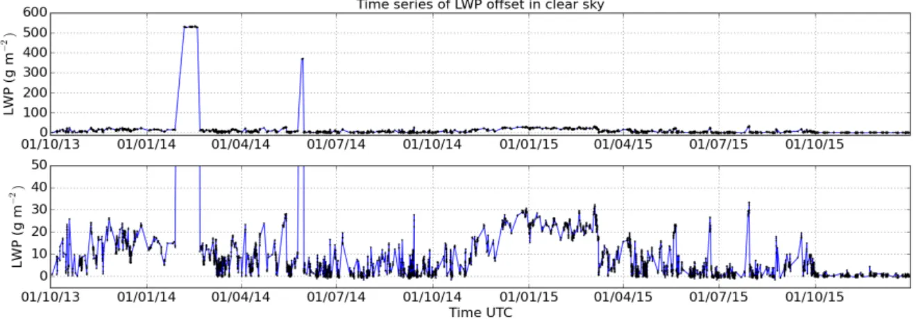
2.5 Liquid water path . . . 38
2.5.1 Microwave retrieval of LWP . . . 38
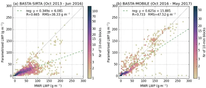
2.5.2 LWP retrieval from radar reflectivity and visibility . . . 42
2.6 Temperature and humidity profiles . . . 43
2.7 Synthesis . . . 46
3 Radiative processes 49 3.1 Published paper: Radiation in fog: quantification of the impact on fog liquid water based on ground-based remote sensing . . . 50
3.2 Parametrising the radiative processes . . . 76
3.2.1 LW radiation . . . 77
3.2.2 SW radiation . . . 79
3.4 Synthesis . . . 86
4 Turbulent processes 89 4.1 Submitted paper: Understanding the dissipation of continental fog by analysing the LWP budget using LES and in situ observations . . . 90
4.2 Impact of subsidence . . . 115
4.3 Synthesis . . . 117
5 Dissipation scenarios 119 5.1 45 days with fog at sunrise: Dissipation scenarios and seasonality . . . 119
5.2 Model of critical fog LWP . . . 122
5.3 Conceptual model of fog LWP budget and CTH development . . . 129
5.3.1 The LWP equation and general assumptions . . . 129
5.3.2 Surface turbulent heat fluxes . . . 132
5.3.3 Entrainment . . . 134
5.3.4 Subsidence . . . 139
5.3.5 Deposition . . . 140
5.4 Statistics of all the morning fog events . . . 144
5.4.1 Distribution of values in the conceptual model . . . 144
5.4.2 Diurnal cycle in the conceptual model . . . 146
5.4.3 Fog thickness and development . . . 148
5.5 Case studies . . . 150
5.5.1 Two fog events in November and February . . . 150
5.5.2 Two fog events near winter solstice . . . 155
5.5.3 Two contrasted events in October 2014 . . . 158
5.6 Uncertainty sources in the conceptual model . . . 161
5.6.1 Radiative processes . . . 162
5.6.2 Surface fluxes . . . 162
5.6.3 Entrainment velocity and entrainment loss . . . 163
5.6.4 Subsidence . . . 167
5.6.5 Deposition . . . 167
5.7 Synthesis . . . 167
6 Conclusions and outlook 171 6.1 Observed patterns in continental fog dissipation . . . 171
6.2 Understanding the evolutions of LWP and CTH . . . 172
6.3 Perspectives . . . 176
Table of symbols and acronyms 181
Bibliography 185
Chapter 1
Introduction
1.1 Foreword
Fog is an interesting meteorological phenomenon in many ways. A fog is basically like a cloud, that is a humid airmass containing microscopic, activated water droplets (or, in cold areas, ice crystals). Unlike clouds, however, fog is in direct contact with the Earth’s surface. This opens the possibility for more direct interactions with the surface and vegetation, and with human activities. Due to the scattering of visible radiation by droplets, the visibility is reduced during fog, which is hazardous for traffic, so that cars, ships and airports must take precautions (Tardif and Rasmussen, 2007). In addition to its impact on the visibility, fog has many effects on the environment. In many dry regions, especially near subtropical west coasts such as in Namibia and Chile, fog is an important source of freshwater to the ecosystems, because it occurs much more frequently than rain (e.g. Seely and Henschel, 1998). Using fog-collecting nets, it is even possible to provide freshwater for local populations from fog (Klemm et al., 2012). As the fog acts as a solvent for many atmospheric aerosols and gases, it impacts the atmospheric chemistry and can catalyse chemical reactions (e.g. Boris et al., 2018). Wet deposition of pollutants is more efficient through fog than rain due to the larger droplet surface area and the longer residence time near the surface, where the concentration of pollutants is highest, which can importantly increase the deposition of pollutants where fog frequently occurs (Dollard et al., 1983; Barrie and Schemenauer, 1986).
This thesis is mainly motivated by the impact that fog has on the visibility. The financial and human losses related to fog can be as large as for tornadoes and even storms due to the delays and increased risk of accidents in air, marine and land transportation (Gultepe et al., 2009). In order to manage and plan traffic efficiently according to the meteorological situation, forecasts of visibility are important (Tardif and Rasmussen, 2007). Fog has proven to be a difficult phenomenon to forecast, and current numerical weather prediction models (NWP) often fail to predict the time and location of the formation and dissipation of fog with sufficient accuracy (e.g. Steeneveld et al., 2015). Although the occurrence of fog and haze has decreased in Europe over the last decades, it still remains a frequent phenomenon in many areas of the continent (Vautard et al., 2009; van Oldenborgh et al., 2010). In particular, it occurs often in the Alpine region, such as the Po Valley. Northern Europe has more fog than the Mediterranean, and the winter has overall more fog days than the summer, with the number of days per winter season with visibility below 200 m (2 km) varying from >15 (>75) for some sites in the Alps and Eastern Europe to <3 (<15) in the Mediterranean and north-western United Kingdom, with most of Northern Europe having an occurrence in the middle of these two (van Oldenborgh et al.,
2010).
This thesis aims to advance the understanding of the different physical processes which govern the fog life cycle and lead to its dissipation. We will explore how ground-based remote sensing instru-ments that observe the atmospheric column can diagnose the variability of physical processes that are important for the fog evolution. This introduction chapter elaborates on the precise definition of fog (section 1.2) and gives an overview of the various situations in which fog may occur (section 1.3). The life cycle and key processes for the fog types studied in this thesis are then presented (section 1.4). The objectives of the thesis will be elaborated at the end of the chapter (section 1.5).
1.2 Definition of fog
Fog is defined as the reduction of visibility to below 1 km due to the presence of suspended water droplets in the vicinity of the Earth’s surface (American Meteorological Society, 2017). Thus, two conditions must apply for fog to occur: (1) the reduction in visibility, and (2) that the main reason for this reduction in visibility is the presence of small, suspended droplets. These two aspects of fog are explained in this section.
1.2.1 Visibility
The definition of visibility from American Meteorological Society (2017) is: “The greatest distance in a given direction at which it is just possible to see and identify with the unaided eye 1) in the daytime, a prominent dark object against the sky at the horizon, and 2) at night, a known, preferably unfocused, moderately intense light source”. This definition is by itself rather subjective, since it depends on the human capacity to observe, and a more objective formulation has therefore been developed based on the concept of the contrast between the object and its background (between 0 and 1). Due to the scattering of the light by the atmosphere between the object and the observer, the contrast decreases with distance according to the following formula (Duntley, 1948):
C = C0e−αext·d (1.1)
where C0 is the contrast at close range, C is the contrast at distance d, and αext is the extinction
coefficient of the atmosphere between the object and the observer. For a black object against a white horizon, C0 = 1. The lowest contrast that the human eye is able to discern is conventionally set to
C = 0.05 by the Commission on Illumination (Hautière et al., 2006). This is then used to derive the visibility distance by the Koschmieder formula:
V is =−ln 0.05 αext
= 3.0 αext
(1.2)
Although the theory used to derive this formula depends on several assumptions, such as a homo-geneous, static atmosphere, a flat and diffuse surface, negligible absorption, and the observed object being small compared to the distance to it, the formula has been found to agree well with human observations (Horvath and Noll, 1969). To measure visibility, the quantity which needs to be observed is therefore the extinction coefficientαext of the atmosphere at visible wavelengths. To get below the
1.2.2 Fog v.s. other phenomena that reduce the visibility
The second part of the fog definition specifies that the reduction of visibility is caused by suspended, microscopic droplets. In fact, there are several other ways the visibility may be reduced. These include heavy rain, blowing snow, smoke and sandstorms. Rain is not fog because the droplets are too big and therefore not suspended but falling from a cloud above. Conventionally the separation between cloud droplets and raindrops is at 200 µm, at which the fall speed is 0.7 m s−1 (American Meteorological Society, 2017). Smoke and sand are not fog because they are dry particles and not droplets. Snowflakes are not fog because they are too big and frozen. Although all of these phenomena can give the same effect on visibility as fog, the processes governing them are very different, and they require different approaches to understand and predict.
However, in cold environments fog may also consist of suspended ice crystals, which is referred to as ice fog (American Meteorological Society, 2017). Ice fog usually does not occur unless the temperature is below -10◦C (Gultepe et al., 2007). When fog made of water droplets occurs below 0◦C, the droplets will freeze when depositing on surfaces, so-called icing, and it is referred to as freezing fog.
If the relative humidity has not reached saturation, the hygroscopic aerosols will not activate into droplets, as explained by Köhler theory (Köhler, 1936), but they can still grow sufficiently large to reduce visibility. This phenomenon is referred to as haze, and the unactivated, hydrated aerosols are called haze particles (American Meteorological Society, 2017). Conventionally, it is assumed that the visibility in haze is higher than 1 km and that it only drops to below this threshold when the haze particles activate to droplets. An intermediate situation is referred to as mist, where relative humidity is close to 100 %, but the visibility is not below 1 km (American Meteorological Society, 2017). However, the distinction between fog and haze is not always sharp: the visibility may be reduced to below 1 km even without activation in very heavily polluted situations, such as extreme haze (e.g. Yang et al., 2015). The activation of cloud condensation nuclei (CCN) into droplets may occur at a smaller or larger diameter, typically in the range 1–4 µm, depending on the mass and chemical composition of the CCN (Rogers and Yau, 1989).
In many situations, several types of particles may contribute simultaneously to reduce the visibility. Fog may occur together with rain, and in industrial areas fog or haze may combine with smoke to form smog (American Meteorological Society, 2017). It has also been shown that haze particles may contribute a significant part of the extinction during fog (Elias et al., 2009).
1.2.3 Droplet size distribution
The fog consists of a large number of small water droplets of different sizes, which constitute a droplet size distribution (DSD). Both the droplet number and sizes are important because they affect how the fog interacts with radiation and the microphysical processes which lead to deposition. The initial number and sizes of the droplets depend on the formation mechanism of the fog (how high the su-persaturation becomes) and the aerosol population which acts as CCN (Rogers and Yau, 1989). The distribution may evolve during the fog life cycle, due to the dynamics of the fog, which may lead to the appearance of bigger droplets (e.g. Price, 2011; Dupont et al., 2012).
The DSD is commonly expressed mathematically as a function n(D), defined so that n(D)· dD is the number of particles in a unit volume of air with diameters between D and D + dD. The total
number of cloud droplets is found by integrating over all sizes:
Nc=
Z Dmax
Dmin
n(D)dD (1.3)
whereDminis the conventional threshold separating the droplets from haze particles (typically 2µm).
As mentioned above, the size Dmax which separates cloud droplets from raindrops is conventionally
set to 200µm. However, most instruments that measure the DSD only capture the droplets smaller than 50µm (Guyot et al., 2015). The liquid water content (LWC), i.e. the mass of droplets in a unit volume of air, can be calculated from the DSD as:
LW C = Z Dmax Dmin πρl 6 n(D)D 3dD (1.4)
whereρl= 103 kg m−3 is the density of liquid water.
In the visible part of the spectrum, cloud droplets efficiently scatter the radiation, while they only weakly absorb. The fraction of the radiation incident to the droplet that is scattered (or absorbed) is referred to at the extinction efficiency (Qext). The extinction coefficient is therefore:
αext= Z Dmax Dmin π 4Qext(D)n(D)D 2dD (1.5)
For cloud droplets that are several times bigger than the visible radiation, a good approximation is Qext= 2 so that the extinction coefficient is (Hu and Stamnes, 1993):
αext=
3LW C ρlDef f
(1.6)
whereDef f is the effective diameter, defined as:
Def f ≡ RDmax Dmin n(D)D 3dD RDmax Dmin n(D)D 2dD (1.7) 1.3 Fog types
Fog forms when the air near the surface becomes supersaturated with water vapour, which triggers the activation and growth of droplets to micrometer sizes. Since the saturation vapour pressure increases strongly with temperature, supersaturation of the air may be obtained from a reduction of the air temperature, from an increase in its water vapour content, or from a combination of the two (Rogers and Yau, 1989). There are therefore several meteorological conditions which may result in fog, and fog types have been defined according to the mechanism causing the fog to appear (Gultepe et al., 2007; Tardif and Rasmussen, 2007).
Radiation fog forms when the land surface is cooled through the emission of LW radiation, usually during the night in clear-sky conditions, leading to supersaturation of the air just above the surface (Haeffelin et al., 2010). This fog type is associated with anticyclones above land (Gultepe et al., 2007). The wind has been shown to be a critical factor for the formation of radiation fog; if the wind is too strong, turbulent mixing will dilute the cooling and moistening in a too thick layer for supersaturation to occur, while too little wind may result in dew deposition instead of fog (Zhou and Ferrier, 2008;
Haeffelin et al., 2013).
Another way to cool the airmass to saturation is by lifting. Upslope fog forms when moist air is forced to lift due to topography, and fog is therefore frequent on the upwind slopes of hills and mountain ranges, especially when the wind comes from a moist area, such as the sea (Błaś et al., 2002).
Fog may also form by a gradual lowering of the base of a pre-existing very low stratus all the way to the surface. Previous studies have identified the mechanisms of cloud-top radiative cooling, subsidence, and the moistening of the sub-cloud layer through evaporation of falling drizzle as possible explanation for this lowering of the cloud base (Koračin et al., 2001; Dupont et al., 2012). Another way that fog can form through moistening is through the evaporation of rain during precipitation events, so-called precipitation fog (Tardif and Rasmussen, 2007). If the precipitation is associated with the passage of a warm front, it can also be called frontal fog; the front may induce fog formation both through evaporation of precipitation and by the mixing of the warm and cold airmasses that meet at the front (Gultepe et al., 2007). Fog may also form due to the evaporation of dew from a wet surface due to heating from the sun right after sunrise, which can lead to saturation of the air. This phenomenon is called morning transition fog (Tardif and Rasmussen, 2007).
Advection fog is the result of the advection of a moist airmass above a colder surface. This is typical for fog formation above the ocean. When warm air is blowing over a colder sea surface, the mixing of the air parcels with different temperature can result in saturation, and it is especially frequent in areas of coastal upwelling (Koračin et al., 2014). Conversely, advection fog can also form when cold air is advected above a warmer surface. In high latitudes, this gives rise to a phenomenon called steam fog (Koračin et al., 2014).
This thesis studies fog events observed at the atmospheric observatory SIRTA near Paris (France). This is a continental mid-latitude site, where the fog events are mainly radiation fog or stratus-lowering fog (Dupont et al., 2016). These fog types will therefore be the focus of the rest of this introduction chapter.
1.4 Life cycle of continental radiation fog and stratus-lowering fog
Previous studies on radiation fog have identified that it goes through different evolutionary stages. Often three stages are described: the formation phase, the development phase and the dissipation phase (e.g. Bergot, 2013). During the formation phase, the surface layer is stable with limited vertical mixing, and it reaches saturation due to radiative cooling of the surface, allowing the formation of small cloud droplets. The fog may form as a very thin layer, just above the cold surface, and its horizontal extent is often broken by patches of clear air, due to heterogeneity of surface properties that impact humidity (Gultepe et al., 2007). This layer may remain thin, but often it develops vertically to become 100 m thick or more. This thicker fog will have a significant emissivity so that the radiative cooling is transferred from the surface to the fog top. This cooling at the top will eventually make the initially stable fog layer neutrally stratified, i.e. a saturated adiabatic lapse rate, which enhances vertical mixing (Price, 2011). This transition from "stable fog" to "adiabatic fog" is important for the fog internal dynamics: while the stable fog has little vertical mixing, the adiabatic fog can be strongly coupled between the surface and its top (e.g. Bergot, 2016). The phase of increasing vertical mixing and TKE is what is referred to by Bergot (2013) as the development phase. As the fog thickens, the initial distribution of small droplets is usually modified with the appearance of larger droplets of
Figure 1.1: The physical processes which impact the liquid water of the fog layer. Those marked in blue will typically produce fog water while those marked in red will reduce fog water.
diameters 15–20 µm, which Price (2011) use to define the mature phase of the fog. However, Price (2011) shows that the appearance of the bigger droplets is not always related to the time when the stable temperature profile becomes saturated adiabatic.
Radiation fog does not always start as a thin layer at the surface, though. In many cases it forms at a few tens of metres of altitude, followed by a rapid downward thickening to the surface (e.g. Haeffelin et al., 2016). The large-eddy simulation (LES) study of Mazoyer et al. (2017) explained the elevated fog formation by the presence of obstacles such as trees, which enhances wind-driven turbulence and dew deposition on the surface and vegetation, thereby limiting the humidity close to the ground. The theoretical calculations of Zhou and Ferrier (2008) suggest that very thin radiation fog cannot persist unless the turbulence is very weak: the more wind-driven turbulence is present, the thicker the fog layer must be to persist. Consequently, the saturated layer needs to acquire a certain thickness before the fog may start to form. Stratus-lowering fog differs from radiation fog by already being thick when fog forms at the surface. In this case, the formation phase consists of an interaction between the stratus and the sub-cloud layer instead of the cooling of a stable layer. Dupont et al. (2012) identified the humidification of the sub-cloud layer by evaporation of droplets falling from the cloud base as a key process for the formation of stratus-lowering fog.
Once the fog has formed, several processes affect its profile of liquid water. This is shown schemat-ically in Fig. 1.1. The contact with the surface allows droplets to deposit on the vegetation, both through the terminal fall velocity of the bigger droplets and through impaction on the vegetation and other obstacles. It has been found that the sedimentation process dominates the deposition under very weak wind speed (< 2 m s−1), while impaction is the most important of the two when the wind is stronger (Katata, 2014). The vertical flux of LWC by sedimentation is essential to account for in order to simulate realistic LWC in fog (Brown and Roach, 1976; Bergot et al., 2007). The surface also exchanges heat with the fog. Due to the radiative cooling, the surface is initially colder than the fog in case of radiation fog formation. However, once the fog has become opaque to long-wave (LW) radiation, the surface is sheltered from the radiative cooling, which instead occurs at the fog top (e.g. Haeffelin et al., 2013). Due to heat diffusion from the soil, the surface temperature will typically become higher than the air temperature, so that the surface becomes a heat source rather than a heat sink for the fog (Roach, 1995; Price, 2011). This becomes much more pronounced once the sun has risen, as the surface is then heated also by solar radiation (Brown and Roach, 1976), so that the fog
is heated from below by turbulent sensible and latent heat fluxes.
The cooling from above and heating from below generates turbulence through buoyancy, so that the fog will contain convective structures (e.g. Nakanishi, 2000). The generated turbulence will promote mixing between the fog and the unsaturated air above the fog top, leading to evaporation of fog droplets (Gultepe et al., 2007) and to upward development of the fog top. However, the mixing at fog top is limited by the strong inversion that usually develops due to the cooling of the fog top (Nakanishi, 2000; Price, 2011; Price et al., 2015). Fog droplets will also evaporate as they approach the heated surface below (Nakanishi, 2000). Radiation fog therefore usually dissipates in the morning due to the heating from the surface, so-called fog burn-off (Tardif and Rasmussen, 2007; Haeffelin et al., 2010). The dissipation phase, as characterised by Bergot (2013), involves an intensification in the vertical mixing due to a further destabilisation of the fog layer by the appearance of solar radiation, or alternatively an increase in wind speed. The dissipation phase can also be characterised by an increase in visibility and a reduction of the LWC and droplet sizes near the surface (Maier et al., 2013).
This thesis focuses specifically on the developed phase of the fog layer and the processes that affect its dissipation. Fog dissipation is defined as the increase of visibility to above 1 km due to removal of the droplets at screen level. Note that dissipation therefore does not require a complete evaporation of the cloud; the cloud may be displaced vertically so that it no longer touches the surface. Radiation fog will typically dissipate after sunrise, but there is still an important variability of the time of dissipation (Dupont et al., 2016), and occasionally very persistent fog may last for the whole day (Price et al., 2015). Roach (1995) summarises the mechanisms that can disperse a fog layer in addition to the heating by solar radiation: (1) the appearance of a cloud layer above the fog, reducing the radiative cooling, (2) heating from the soil, more so in autumn than in winter, and (3) an increase in the wind speed, which enhances mixing. These mechanisms of dissipation of fog all act by modifying the balance between the processes controlling the liquid water of the fog (Fig. 1.1). The mechanisms have since been studied using numerical models and observational studies. Bergot (2016) showed with LES simulations that a stronger wind speed favours earlier dissipation, due to the increased turbulence and mixing with the air above. The results of Maronga and Bosveld (2017) indicate that high soil temperature mainly delays fog formation and does not affect dissipation as much. Soil moisture, however, impacts the dissipation time, with drier soil favouring earlier dissipation due to the reduction in latent heat flux (Maronga and Bosveld, 2017). Due to its impact on the fog optical depth and sedimentation rate, the fog droplet number concentration can also affect dissipation time, with fewer and larger droplets favouring earlier dissipation (Maalick et al., 2016; Mazoyer et al., 2017). Falling droplets can cause fog dissipation by collection processes and deposition, but they can also cause lowering of a low stratus cloud base to the ground to form stratus-lowering fog, as studied with Doppler cloud radar by Dupont et al. (2012). Large-scale advection also has impacts on fog dissipation. The observations of Price et al. (2015) show that warm advection can reduce the relative humidity in the air overlying the fog and therefore increase the loss by mixing, which can lead to dissipation. Thus, drying from mixing, contributing to dissipation, can be enhanced by both increase in wind speed and reduction in the relative humidity of the air above. It was found in LES studies (Bergot, 2013, 2016) that dry tongues of air which penetrate the fog from above, cause a large horizontal spread in the liquid water path (LWP) during the dissipation phase of fog, so that the time of fog dissipation can be variable in the horizontal even if the surface forcing is homogeneous. Circulations at the horizontal edge between fog and clear air, driven by temperature gradients, can be an important mechanism for dissipating the
fog, as observed by Price et al. (2015). However, they also found that such circulations at the fog edge can drive a rapid expansion of the fog layer when the clear air is close to saturation.
1.5 Context and objectives for the thesis
One reason that fog is challenging to predict is that it is a threshold phenomenon governed by many small-scale processes; subtle differences in these processes can impact the fog formation or dissipation (e.g. Zhou and Ferrier, 2008; Haeffelin et al., 2013). In numerical weather prediction (NWP) models, the small-scale processes must be parametrised. Bergot et al. (2007) compared the fog prediction by single-column models of fog and found important sensitivity of the results to which parametrisa-tions were used for droplet sedimentation and soil-atmosphere interacparametrisa-tions, and also to the correct representation of the nocturnal inversion.
As a supplement to NWP, statistical models are developed for sites for which fog forecasts are needed, in particular airports. The models relate the visibility to other meteorological observations, such as temperature, relative humidity, wind speed and cloud cover. Based on a long time period of continuous measurements, conditions preceding fog formation or dissipation can be statistically identified and give a probabilistic short-term forecast of the visibility (e.g. Pasini et al., 2001) or the time of fog formation (e.g. Fabbian et al., 2007). Most of the investigations have focused mainly on observations of near-surface conditions. These are easier to observe with ground-based instruments than the properties higher up in the fog. However, since once the fog has formed, many of the processes occur near the fog top, it is important to observe the whole vertical profile of the fog layer to understand its evolution and dissipation.
Ground-based remote sensing instruments such as cloud radars and microwave radiometers (MWR) are well suited for continuously measuring properties of the vertical profile of fog and clouds. Many algorithms have been developed, based on one or several instruments, to retrieve geophysical parame-ters of clouds from the observations, such as the LWP from the MWR (Rose et al., 2005), and LWC, ice content or particles sizes from the cloud radar, with or without combining it with the MWR (e.g. Dong and Mace, 2003; Delanoë et al., 2007; Martucci and O’Dowd, 2011). These instruments are currently becoming less expensive and with higher performance, and more commonly deployed on sites of interest. For example, the ceilometer, which is traditionally only used for cloud-base detection, is being improved to give information about the vertical profile of extinction, which can be used to track the hygroscopic growth of aerosols that may lead to elevated radiation fog formation (Haeffelin et al., 2016). The systematic use of observations from these remote sensing instruments is further being facilitated by the efforts to establish standardised conventions for quality control, calibration routines, data file formats and the sharing of data between institutions and between countries. In Europe, such collaboration is currently undertaken by the project ACTRIS (www.actris.eu). By retrieving properties of the whole atmospheric column in real-time, the remote sensing instruments have a great potential for contributing to weather forecasts. The observations may either be directly used to anticipate the evolution in the next hours (nowcasting) or they can be assimilated in NWP to improve the initial state of these models. Recent studies have shown that certain short-term NWP forecasts can be improved by assimilation of MWR temperature and humidity profiles (Caumont et al., 2016).
This thesis aims (1) to improve the understanding of the physical processes that play a role in fog dissipation, and (2) to investigate how the observations from ground-based remote sensing instruments
can be used to understand and possibly anticipate the fog dissipation. We have chosen to focus particularly on the fog events that persist until sunrise, on how they evolve during the daytime until their dissipation. We further focus on the local processes, by which we mean the processes that occur in the vertical column of the atmosphere on a small horizontal scale, and which do not depend on horizontal advection or heterogeneities. The investigations will be centred on the following questions: • How much does each of the local processes contribute to the liquid water budget of the fog, in
various conditions?
• What is the impact of the variability of the properties at and above the fog top on the liquid water budget and dissipation of the fog?
• What information can be derived from the cloud radar and MWR measurements about the current state of the different fog processes?
• How is the dissipation of fog related to the evolution of its LWP and its thickness?
• To what extent can the observed evolution of the fog be attributed to the local processes, and how much must rather be attributed to advection and other non-local effects?
To answer these questions, a dataset of 7 years of fog events at the SIRTA observatory is studied. The various geophysical properties that we retrieve from observations and their variability are presented in chapter 2. Numerical modelling tools are thereafter used to understand what impact the observed variability has on different processes. In chapter 3, a comprehensive radiative transfer code is applied to study the radiative processes in fog and quantify their impacts on the LWP of the fog through heating and cooling. This chapter incorporates our published paper on this topic (Wærsted et al., 2017, hereafter W17). The dynamical processes, including surface–fog interactions and the mixing between the fog and the air above, are studied using high-resolution LES in chapter 4, which contains our paper on this topic which was submitted in July 2018 (Wærsted et al., 2018, hereafter W18). Chapters 3 and 4 allow a quantitative analysis of the importance of various local processes for the evolution of the fog LWP and its dissipation. In chapter 5, these results are applied to analyse a much larger number of fog events (45) through a conceptual model. The analysis aims to quantify the variability of the impacts of the different processes among the observed events and to explain some of the differences we observe in the evolution and time of dissipation among the events. Finally, the conclusions are presented in chapter 6.
Chapter 2
Observed properties of fog events
This chapter presents the instrumentation used in this study and the various fog properties that can be retrieved from them. It also presents statistics of these properties from the large number of fog events observed on the SIRTA observatory.
2.1 Observational site SIRTA
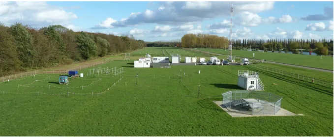
SIRTA (Site Instrumental de Recherche par Télédétection Atmosphérique) is a multi-instrumental atmospheric observatory located 20 km south of Paris at the university campus of École Polytechnique, where a large number of atmospheric variables have been continuously recorded since 2002 (Haeffelin et al., 2005). Thanks to the elevated number of fog events occurring there each winter, this site is suited for fog observational research, which has been a scientific priority for the site since the ParisFog project started in 2006 (Haeffelin et al., 2010). Table 2.1 presents the instruments used in this thesis to study fog. Nearly all of these instruments are located in the main facility of the SIRTA observatory, hereafter referred to as "the platform", which is located on a grass field between a narrow wood to the north and a small lake to the south (Fig. 2.1). The larger surroundings are characterised by a patchwork of university buildings, small woods, agricultural and sports fields, and suburban houses.
Standard meteorological measurements (2-m temperature and humidity, 10-m wind speed, surface pressure) are recorded continuously at the platform. In addition, there are six levels of temperature
Instrument Measured quantity Vertical range and resolution Temporal resolution Available from Remote sensing 95 GHz Doppler FMCW cloud radar (LATMOS, BASTA) Reflectivity (dBZ), Doppler velocity (m s−1) RA 0-6(12) km, RE 12.5(25,100,200) m 12 s July 2013 14-channel microwave radiometer (MWR) (RPG HATPRO)
LWP (g m−2) Integrated 1 min Feb 2010
IWV (kg m−2) Integrated 1 min Feb 2010
Temperature profile (K) RA 0–10 km, 4–5 deg. of freedom ≈5 min Feb 2010 Humidity profile (g m−3) RA 0–10 km, 2 deg. of freedom ≈5 min Feb 2010 905-nm ceilometer (Vaisala
CL31)
Attenuated backscatter (m−1 sr−1)
RA 0–7.6 km, RE 15 m 30 s Dec 2010 Sodar (Remtech SFAS) Wind speed profile (m s−1) RA 10–200 m, RE 5 m 10 min Nov 2015† Granulometers
Fog monitor (DMT FM-120) Droplet concentration (cm−3) in 30 size bins (2–50µm) At 4? m 1 s Oct 2013 Aerosol counter (Meteomodem LOAC) Particle concentration (cm−3) in 19 size bins (0.2–50? µm)
Tether balloon profiles 0–300 m 1 s IOP Surface layer state
550-nm scatterometer (Degreane DF20+) Visibility (m) At 3 m 60 s Feb 2010 550-nm scatterometer (Degreane DF320) Visibility (m) At 4 m 60 s Oct 2013 875-nm scatterometer (Vaisala PWD22) Visibility (m) At 20 m 60 s Oct 2013 Thermometers (Guilcor PT100)
Air temperature (K) At 1,2‡,5,10,20,30 m 60 s Sept 2011 Barometer (Vaisala PTB110) Surface pressure (Pa) At 2 m 60 s 2005 Rain gauge 3070
(Precis-Mecanique)
Precipitation rate (mm h−1) At 2? m 60 s 2005 Sonic anemometers
(METEK)
Mean wind speed (m s−1), momentum flux (m2s−2)
At 10,30 m 10 min 2007
Ground and soil state
Thermometer (unsheltered) Skin temperature (K) At ground level 60 s Jan 2014(?) Soil thermometer (Guilcor) Soil temperature (K) At 5,10,20,30,50,100 cm depth 60 s Feb 2007 Soil moisture sensor
(ThetaProbe)
Soil moisture (m−3m−3) At 5,10,20,30,50,100 cm depth 60 s Feb 2007 Surface energy budget
Pyranometers (Kipp & Zonen CMP22)
Down- and upwelling irradiance in solar spectrum (W m−2)
At 10 m 60 s Apr 2012
Pyrgeometers (Kipp & Zonen CGR4)
Down- and upwelling irradiance in terrestrial spectrum (W m−2)
At 10 m 60 s Apr 2012
Heat flux sensor (Hukseflux HFP01SC)
Soil heat flux (W m−2) At 5,20,100 cm depth 60 s Jan 2014 GILL sonic anemometer and
LI-7200 infrared gas analyser
Sensible and latent heat flux (W m−2) At 2 m 10 min Nov 2015† Radiosondes (M10, Météo France, Trappes) Temperature (K), relative humidity (%) RA 0–30 km, RE≈ 5 m 12 h 1999?
Table 2.1: Instruments used in this thesis for the study of fog. All the instrument apart from the radiosondes are located on the platform shown in Fig. 2.1. †The sodar and surface turbulent flux station were deployed for a longer period, but are only used for November 2015 in this study. ‡There is a separate thermometer at 2 m which is deployed from 2005.
and humidity measurements on the 30-m mast shown in Fig. 2.1. Wind speed is also measured by sonic anemometers at 10 m and 30 m, obtaining also the momentum flux, which allows the calculation of aerodynamic resistance (see section 5.3.2). Visibility is measured at screen level (3 or 4 m) and at 20 m.
The different terms of the surface energy budget are also measured. Two pairs of pyrano- and pyrgeometer measure global upwelling and downwelling short-wave (SW) and long-wave (LW) radiative flux at 10 m, and turbulent sensible and latent heat fluxes are measured at 2 m with the eddy covariance method using a GILL sonic anemometer and an LI-7200 closed-path infrared gas analyser. The ground heat flux is measured at 5, 20 and 100 cm depth. Soil temperature and moisture are measured at
these and three additional levels, and an unsheltered thermometer in the grass measures surface skin temperature.
Full atmosphere profiles of temperature and humidity are available from radiosondes launched from the Météo-France station Trappes twice a day, at around 11 and 23 UTC. Trappes is located 15 km to the west of SIRTA and is 12 m higher above sea level.
The fog monitor FM-120 (Droplet Measurement Technologies) is deployed at SIRTA every winter season since 2013. This instrument counts and sizes individual droplets using a forward scattering probe inside a small measurement chamber, which samples a steady flow of air using an active ventila-tion. Particles are categorised into 30 size bins in the range 2–50µm (in diameter), which are mostly droplets. From October 2014, it is equipped with a swivel, which ensures that the air inlet faces the wind direction, giving a more reliable sampling of droplets.
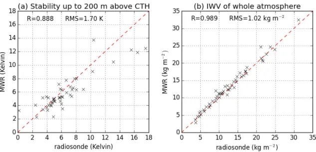
Several remote sensing instruments useful for fog observations are also deployed at the platform. A Vaisala CL31 ceilometer operating at 905 nm provides a vertical profile of (attenuated) light backscat-ter with 15 m resolution (Kotthaus et al., 2016). This wavelength is highly sensitive to cloud droplets, giving reliable detection of clouds. Since the cloud rapidly attenuates the ceilometer beam, further characterisation of the cloud profile above the cloud base is performed by the 95 GHz cloud radar BASTA (Delanoë et al., 2016,http://basta.projet.latmos.ipsl.fr/), which is deployed in a ver-tically pointing position. Because this cloud radar uses the frequency-modulated continuous wave (FMCW) technique, rather than pulses, its components are less expensive than traditional cloud radars. BASTA is suitable for fog studies due to its high resolution (12.5 m) and small blind zone (40–60 m) compared to many other cloud radars. The prototype of BASTA has been operating at SIRTA since 2010, but its high-resolution product is only available from the summer 2013. In addition to the high-resolution mode, the cloud radar has three more modes with higher sensitivity but larger blind-zone and smaller vertical resolution, all of which give one profile every 12 s. In this thesis, we use the 100-m resolution mode for detecting clouds above the fog (or the 200-m mode in W17), while the 12.5-m mode is used for observing the fog. Finally, the 14-wavelength MWR HATPRO provides brightness temperature measurements in 7 oxygen and 7 water vapour bands. The vertically integrated liquid water path (LWP) and integrated water vapour (IWV) of the whole atmospheric column, as well as rough profiles of temperature and humidity up to 10 km can be retrieved from these measurements (Rose et al., 2005).
2.2 Fog events observed at SIRTA
Most of the instruments used in this thesis have been measuring at SIRTA almost continuously since 2010 (Table 2.1). This long time series captures a large number of fog events, which is valuable for a statistical study of the fog life cycle. However, since high-resolution cloud radar data is only available from October 2013, a particular focus will be given to the fog events occurring after this.
Most of the analysis performed in this thesis is based on averages of observations in 10-minute blocks. It is convenient to use blocks to get the same times for each observed quantity. The sample size of 10 min is chosen because most of the observations are given at least once every 10 min (Table 2.1). Although the spacing of observations is not always completely even, no weighting of observations are done when averaging.
Fog presence is detected using the visibility measured at 3 or 4 m altitude (the df20+ instrument is used until 30 Sept 2013, and the DF320 thereafter). If at least half of the visibility measurements
Figure 2.2: Fog events detected during seven winter seasons by visibility. The fog events are marked in blue, while red lines indicate periods where visibility data are missing. For the first three winter seasons, we use the visibility meter DF20+ and for the last four DF320 (see Table 2.1).
are below 1 km in a 10-min block, it is considered a fog block. No distinction is made between fog and other phenomena that could reduce the visibility to below 1 km; however, the only other possibility is heavy rain, since sandstorms, snowstorms or extreme haze does not occur at SIRTA. Most of the fog events are observed by the ceilometer, which confirms that a cloud base is present. Fog events are defined using a 3-of-5 rule similar to the algorithm of Tardif and Rasmussen (2007), but with 10-min blocks rather than hourly measurements. A positive construct is defined as a sequence of 5 blocks where the middle block and at least 2 others are fog blocks. A negative construct is defined as a sequence of 5 blocks where the middle block is a fog block, but less than 2 of the others are. A fog event begins with the first fog block within a positive construct. It ends when a negative construct or 3 consecutive non-fog blocks are detected; the end of the fog is then set to the last fog block in the previous positive construct. After detecting fog events in this way, we merge neighbouring events that are closer than 60 min. Finally, events shorter than 60 min are discarded.
This fog detection algorithm identifies 250 fog events in the period 1 Oct 2010 – 30 Sept 2017, of which 218 occur in the winter half-year (October to March). In the period 1 October 2013 – 30 September 2017, which is the main focus of the thesis, there are 129 fog events. 114 of these have data from both the cloud radar BASTA and the MWR HATPRO. Figure 2.2 shows the occurrence of fog events during the seven winter seasons. It is clear that the fog events are not evenly distributed, but often occurring in clusters lasting up to a week. This clustering is probably related to periods where synoptic weather conditions are favourable for radiation or stratus-lowering fog formation. Unfortu-nately, visibility data are missing in some extended periods, especially during the mid-winter of the two first seasons (Fig. 2.2), so that we likely are missing some fog events.
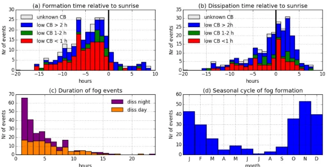
Figure 2.3: Fog events detected from 1 Oct 2010 to 30 Sept 2017: (a) Time of formation and (b) time of dissipation relative to sunrise. The different colours mark how long a cloud base is present below 400 m before formation (in a) and after dissipation (in b), ignoring cloud absence lasting less than 30 min. For some events it is unknown, due to missing ceilometer data. (c) Duration of the fog events, for those dissipating in night and in day. (d) The number of fog events forming in each month.
Figure 2.3a shows the distribution of fog formation time relative to sunrise among the 250 events. The colour classification corresponds to the time that a low cloud base is present before fog formation time (for detection of cloud base, see section 2.3). The fog events for which it is 2 h or more can be considered as stratus-lowering fog events (83 events), while the others are likely radiation fog events (150 events). Fog most frequently forms in the last 5 hours of the night (Fig. 2.3a), which is consistent with previous studies of radiation fog (Tardif and Rasmussen, 2007; Dupont et al., 2016), because radiative cooling accumulates throughout the night. There are also a few cases of formation after sunrise, but these are mainly due to stratus-lowering. Dissipation is most frequent around sunrise or up to 4 h after sunrise (Fig. 2.3b), as expected for radiation fog and stratus-lowering fog (Tardif and Rasmussen, 2007). There is also an important number of fog events which dissipate at night. These are significantly shorter in duration than those dissipating in the day: while more than half of the fog events dissipating at night last less than 3 h, the same holds true for only a quarter of those dissipating in day (Fig. 2.3c). Figure 2.3b also distinguishes the events where a low cloud remains for more than 1 h and more than 2 h after dissipation. It is common that a cloud remains for at least 2 h (at least half of the events), indicating that the fog usually dissipates at ground level prior to the complete dissipation of the cloud. This dissipation after sunrise by lifting of cloud base is also the behaviour found in several LES studies (e.g. Nakanishi, 2000; Bergot, 2013; Mazoyer et al., 2017). Finally, Fig. 2.3d shows that there is a strong seasonal cycle in the occurrence of fog, with most of the events in October–February, which is typical for northern Europe (section 1.1).
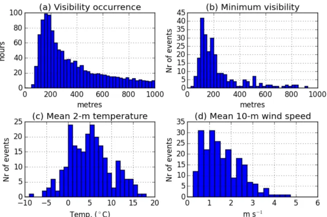
Figure 2.4 shows the variability of the surface meteorological variables during the fog events. The visibility usually reaches a minimum value in the range 100–300 m (Fig. 2.4b), but with important duration of higher visibilities (Fig. 2.4a). The temperature has a large range of variability, with some events warmer than 15 ◦C and several events with temperatures below 0◦C, while most of the events
Figure 2.4: Surface meteorological conditions during the 250 fog events observed during Oct 2010 – Sept 2017 (based on 10-min blocks within each fog event): (a) duration of 10-min median visibility during all fog events (excluding blocks with visibility above 1 km); (b) minimum value of the 10-min median visibility in each fog event; (c) mean temperature during each fog event; (d) mean wind speed (from sonic anemometer at 10 m) during each fog event.
have temperature in the range 0–10◦C (Fig. 2.4c). The 10-m wind speed (Fig. 2.4d) is usually below 3 m s−1 with a few events having higher wind speed (up to 5 m s−1). This is in agreement with previous studies finding that radiation fog typically forms when wind speeds is below 3 m s−1 (e.g. Menut et al., 2014), and the average values of 1.5 and 1.8 m s−1 during radiation fog and stratus-lowering fog, respectively, found by Dupont et al. (2016).
2.3 Cloud base and top
The cloud base height (CBH) is detected using the ceilometer. Following Haeffelin et al. (2016), it is set to the first gate in the profile where the attenuated backscatter signal exceeds the threshold of 2 ·10−4m−1sr−1. The visibility at 3 or 4 m is used to detect when the CBH is at the surface (fog): when the visibility is less than 1 km, the CBH is set to 0 m. While the ceilometer is excellent for detecting the base of the cloud, since its laser beam interacts very strongly with droplets, the rapid attenuation of the signal means it cannot observe the whole cloud profile. Here the cloud radar BASTA comes of use. By using microwave radiation, the signal interacts only weakly with the clouds and is able to penetrate even thick clouds to give a full atmospheric profile of cloud occurrence.
The backscattered signal from hydrometeors which are hit by the cloud radar beam increases strongly with the size of the particle. When observing liquid droplets, the backscattered power is
proportional to the sixth power of the diameter1 (Rogers and Yau, 1989). The range-corrected signal received by the cloud radar can therefore be used to estimate the radar reflectivity, defined as:
Z = Z ∞
0
n(D)D6dD (2.1)
Z has units of mm−6 m−3, but is usually given in dB scale, with unit dBZ =10· log
10(Z). The cloud
radar BASTA retrieves this product, assuming the target are cloud droplets. The values of Z are studied in section 2.4.2. For ice clouds, a similar relationship holds, but the signal is slightly weaker for similar sized particles due to ice having a smaller refractive index than water (Rogers and Yau, 1989).
To detect the cloud top height (CTH), we use the automatic signal detection analysis of the cloud radar software, which is based on the signal-to-noise ratio (Delanoë et al., 2016) and evaluates whether each measurement is good signal or noise. In a 10-min block, if at least half the measurements at a radar gate is considered good signal by this analysis, that gate is assumed to have a cloud signal. Searching upwards from the detected CBH, the CTH is set to the base of the first gate without cloud signal, provided that the following 2 gates do not have cloud signal either, and that a cloud signal was detected in the gate below. Four examples of the detection of cloud base and top are shown in Figs. 2.5–2.8.
Since the backscattered signal increases with the particle diameter in the sixth power, the signal from clouds containing only small droplets may be too weak to be detected by the cloud radar. Due to the dispersion of the radar beam, the sensitivity threshold (i.e. the lowest value of Z that can be detected) increases proportionally with the square of the range (i.e. the distance between the cloud radar and the target), which means an increase of 6 dBZ for every doubling of the range. The sensitivity at 1 km range of the cloud radar prototype operating at SIRTA until 2016 (BASTA-SIRTA) is about -27.5, -32, -38 and -41 dBZ with the 12.5-m, 25-m, 100-m, and 200-m modes, respectively, although it may vary with the atmospheric conditions (Delanoë et al., 2016). However, from October 2016 to June 2017 a more sensitive prototype was deployed (MOBILE), and from June 2017 BASTA-SIRTA was again deployed but with an improved sensitivity similar to that of BASTA-MOBILE. The improvement in sensitivity is at least 10 dBZ (Delanoë et al., 2016).
The 12.5-m mode of the cloud radar is used for cloud top detection, because it has the highest vertical resolution and the smallest blind-zone. Nevertheless, the 3 lowest gates cannot be used, and the following 2 gates almost always have some signal even if there is no cloud, due to the noise effect in the 3 first gates actually extending to a lesser extent into these next gates, making it hard to automatically distinguish a weak cloud signal from the instrumental noise (see examples in Fig. 2.5a, Fig. 2.7a). Therefore, the estimated fog top has a lower limit of 60–80 m when retrieved by the cloud radar. However, we may use the visibility meter at 20 m to determine whether the fog top is below 20 m or not. If the median visibility measured at 20 m is higher than 1 km while fog is detected below, we know that CTH < 20 m. In these cases, CTH is set to 10 m (in case of cloud base detected at 7.5 m, it is set to 14 m). An example is the early stages of the fog on 27 Oct 2014, when the visibility at 20 m stays well above 1 km while the 4-m visibility shows periods of fog (Fig. 2.5d). The cloud radar signal may sometimes also detect signals which are not cloud, such as after fog dissipation on 27 Oct 2014; after 9:30 UTC it is clear from the ceilometer that there is no cloud below 500 m (Fig.
1
For raindrops that are not much smaller than the cloud radar wavelength (3 mm), this power-law is not valid, although the signal still increases with drop size
Figure 2.5: Ti me series of the fog ev en t on 27 Oct 2014. V ertical lines mark fog formation and dissipation times (see section 2.2). (a) The profile of radar reflectivit y (Z) and (b) Doppler v elo cit y from the cloud radar (sho w ing only data remaining after noise filtering), (c) the atten uated bac kscatter of the ceilometer, (d) L WP retriev ed b y the MWR (see section 2.5.1) and visibilit y at 4 m and 20 m , and (e) the retriev ed CBH and C TH. Figure 2.6: Time se ries of observ ations an d retriev al o f cloud b ound-aries for the fog ev en t on 30 No v 201 4. See Fig. 2.5 for a further explanation.