2006 — Development of advanced algorithms for displacement, velocity and pressure control of electro-hydraulic systems

(1)

A THESIS SUBMITTED TO

ÉCOLE DE TECHNOLOGIE SUPÉRIEURE

IN FULFILLMENT OF THE REQUIREMENTS FOR THE DEGREE OF MASTER

IN MECHANICAL ENGINEERING M.Eng.

BY JAHO SEO

DEVELOPMENT OF ADV ANCED ALGORITHMS

FOR DISPLACEMENT, VELOCITY AND PRESSURE CONTROL OF ELECTRO-HYDRAULIC SYSTEMS

MONTRÉAL, APRIL 5, 2006

(2)

M. Jean-Pierre Kenné, director ofresearch

Mechanical Engineering Department at École de technologie supérieure

M. Ravinder Venugopal, co-director of research President of Sysendes Inc.

M. Antoine Tahan, professor and president of the jury

M. Martin Viens, member of the jury

THIS THESIS WAS DEFENDED BEFORE THE JURY AND PUBLIC ON MAR CH 1, 2006

(3)

JaHo Seo Sommaire

Les systèmes hydrauliques sont largement utilisés dans plusieurs secteurs industriels, particulièrement dans les applications qui exigent des forces ou des couples élevés. Bien que ces systèmes hydrauliques aient des composantes mécaniques relativement simples, ils sont pourtant caractérisés par des dynamiques non linéaires, plus spécifiquement, une relation en racine carrée entre la pression différentielle qui entraîne 1' écoulement du fluide hydraulique et la vitesse de 1' écoulement ou débit.

La plupart des contrôleurs industriels disponibles sur le marché utilise des commandes de type PID pour contrôler la force, la vitesse et le déplacement dans les systèmes hydrauliques. Cependant, leur performance est limitée à cause de la nature non-linéaire des ces systèmes.

Dans cette étude, nous choisissons la méthode de linéarisation de rétroaction de façon à surmonter les effets non linéaires inhérents au système. En utilisant cette théorie de commande non-linéaire, nous nous proposons de développer des contrôleurs avancés pour la commande du déplacement angulaire, de la vitesse angulaire et de la pression des actuateurs hydrauliques rotationnels. Parallèlement, nous nous proposons de valider la performance élevée des contrôleurs basés sur la linéarisation de rétroaction grâce à des essais de simulation et à des mesures expérimentales sur un banc d'essais hydrauliques.

(4)

JaHo Seo Abstract

Hydraulic motion drives are widely used in several areas of industry, especially in applications that require high forces or torques. While typical hydraulic systems have relatively simple mechanical components, they are characterized by nonlinear dynamics, specifically, a square-root relationship between the differentiai pressure that drives the flow of the hydraulic fluid and the flow rate.

Most commercially available industrial controllers use PID control for force, velocity and displacement control in hydraulic systems; however, their performance is limited due to the nonlinear nature of these systems.

In this study, we use the technique of feedback linearization method to overcome the effects of the nonlinearity. Using this nonlinear control approach, we develop advanced controllers for angular displacement, angular velocity and pressure control of a rotational hydraulic drive, and test the performance of feedback linearization based controllers through simulation & experimental testing on a hydraulic test-bench.

(5)

dans le domaine de la commande en raison des avantages tels que la compacité, le rapport force/masse élevé et la précision. Cependant, la caractéristique non-linéaire du système hydraulique limite la performance du contrôleur, basé sur la méthode linéaire traditionnelle, comme PID, d'où une théorie avancée et robuste considérant la non-linéarité est nécessaire. La méthode de linéarisation de rétroaction pourrait être une alternative pour satisfaire ce besoin.

Dans notre étude, l'objectif principal de ce projet est de développer des algorithmes avancés pour la commande du déplacement, de la vitesse et de la pression des systèmes hydrauliques rotationnels en utilisant la théorie de linéarisation de rétroaction. En même temps, notre projet contribuera à la réalisation des objectifs spécifiques suivants :

• Développer un modèle mathématique décrivant la dynamique du système.

• Développer des algorithmes de commande ( c.-à-d. contrôleur PID et contrôleur basé sur la linéarisation de rétroaction) en utilisant le modèle mathématique proposé.

• Implanter les algorithmes de commande du système développé sur un banc d'essai et comparer les performances des contrôleurs développés.

Pour réaliser les objectifs mentionnés ci-dessus, nous avons présenté les séquences et méthodes d'étude dans l'ordre suivant:

1. Description du système électrohydraulique

Notre système de commande pour cette recherche se compose essentiellement de deux servo-valves électrohydrauliques, qui commandent le mouvement d'actionneur hydraulique et le couple de charge du système respectivement. L'huile est retournée au réservoir d'huile à la pression atmosphérique par la servovalve.

(6)

2. Développement d'un modèle mathématique permettant de représenter la dynamique du système étudié.

3. Le contrôleur PID adapté au système linéarisé sera conçu en appliquant la méthode de Ziegler-Nichols. Ce contrôleur PID sera appliqué respectivement au système linéarisé et non-linéaire pour la simulation. La simulation en boucle fermée dans deux conditions d'entrée en échelon unité et sinusoïdale sera faite par MA TLAB/ Simulink. Les résultats obtenus par cette simulation en boucle fermée contribueront à identifier la performance limitée du contrôleur PID appliqué au système non-linéaire.

4. Le développement de chaque contrôleur pour la commande du déplacement angulaire, de la vitesse angulaire et de la pression de charge du système non-linéaire en utilisant la technique non-linéaire de type linéarisation de rétroaction. En outre, chaque contrôleur appliqué au système non-linéaire sera validé par la simulation en boucle fermée à 1' aide de MATLAB/Simulink et sa comparaison avec le contrôleur PID de l'étape 3 sera effectuée en fonction de sa performance.

5. La commande en temps réel pour l'essai expérimental de chaque algorithme de commande ( c.-à-d. commande de type PID et commande par linéarisation de rétroaction) proposé ci-dessus sera faite un utilisant le banc d'essai du LITP (Laboratoire d'intégration des technologies de production). Simultanément, le travail à l'étape 5 inclut la comparaison de la performance entre le contrôleur basé sur la linéarisation de rétroaction et le contrôleur PID.

Dans cette recherche, le principal processus parmi les procédures mentionnées ci-dessus est la comparaison de la performance de chaque contrôleur par les simulations de deux types faites aux étapes 4 et 5. Par cette comparaison, nous avons l'intention d'arriver à la conclusion que la stratégie de linéarisation de rétroaction est très adaptée pour concevoir un contrôleur avec la performance de poursuite plus élevée et stable pour la

(7)

commande du déplacement angulaire, de la vitesse angulaire et de la pression de charge dri système hydraulique rotationnel en surmontant la limitation du contrôleur PID.

Pour l'organisation de cette thèse, mentionnons que cette recherche se compose de 4 principales parties.

Dans le chapitre 1, à travers une revue de littérature, nous donnons une idée générale et un aperçu sur 1' état de 1' art dans le domaine de recherche, axé sur la commande des systèmes électrohydrauliques.

Le deuxième chapitre nous permet de comprendre des systèmes asservis par la modélisation et explique comment installer l'environnement expérimental pour notre système électrohydraulique.

Dans le troisième chapitre, nous validerons la réponse de chaque système ( c.-à-d. le déplacement angulaire, la vitesse angulaire et la différence de pression de la charge) après la linéarisation par la simulation en boucle ouverte avec MA TLAB/Simulink. En outre, nous présentons la procédure pour développer le contrôleur PID par la méthode de Ziegler-Nichols et le contrôleur par la théorie de linéarisation de rétroaction. Les résultats comparatifs concernant la performance de poursuite de chaque contrôleur appliqué au système non-linéaire seront analysés par la simulation en boucle fermée avec MA TLAB/Simulink.

Au quatrième chapitre, l'analyse comparative des performances de chaque contrôleur sera faite par la simulation en temps réel en utilisant le banc d'essai du LITP. Finalement, L'évaluation et la conclusion générale pour la stratégie non-linéaire appliquée dans notre étude seront présentées.

(8)

I would like to thank Dr. Jean-Pierre Kenné, my director for his sincere advice, helpful guidance, and devoted endeavor to provide me with the best environment for my research. I am also grateful to Dr. Ravinder V enugopal, my co-director for his systematic instruction and outstanding teaching regarding the theoretical and empirical approach to research. In addition, I thank Mr. Kaddissi who, in spite of his busy schedule, offered advice related to my experiment.

I would also like to thank Mr. Charlot for his friendship and heart felt consideration for my. persona! affairs as weil as my academie studies. I equally give thanks for the camaraderie and help I have received from ali members of LITP (Laboratoire d'intégration des technologies de production).

Without the steady understanding, devotion, support and constant love of my wife, Y un Hee Lee, it is needless to say that this accomplishment and honor could not have been imagined.

In addition, I deeply appreciate the encouragement, financial and spiritual support and unflagging trust of my parents, sisters and brother.

(9)

Finally, 1 would sincerely like to express my gratitude for my lord Jesus Christ, my dear Father and two Sisters of the Korean Community Catholic church.

(10)

SOMMAIRE ... iii

ABSTRACT ... ~ ... .iv

RÉSUMÉ DU MÉMOIRE EN FRANÇAIS ... v

ACKNOWLEDGEMENTS ... viii

TABLE OF CONTENTS ... x

LIST OF TABLES ... xii

LIST OF FIGURES ... xiii

NOMENCLATURE ... xvii INTRODUCTION ... ! CHAPTER 1 1.1 1.2 1.3 1.4 1.5 CHAPTER2 2.1 2.2 2.2.1 2.2.2 2.2.3 2.2.4 2.2.5 2.3 CHAPTER3 3.1 3.2 3.2.1 3.2.2 3.2.3 LITERA TURE REVIEW ... 5

Advantages and disadvantages ofElectro-hydraulic servo-system ... 5

Hydraulic drive control approaches ... 6

Feedback linearization approach ... 8

Modeling and experimental setup ... 9

Simulation and real-time control.. ... ! 0

MODELING OF ELECTRO-HYDRAULIC SYSTEM ... l2 Setup ofElectro-Hydraulic System ... l2 Modeling ofElectro-Hydraulic System ... 14

Servo-valve opening area and input command variables ... l4 Load pressure difference variable ... 15

Angular velocity variable ... 19

Sigmoid function ... 19

State Space Model ... 21

Linearization ... 23

CONTROL ALGORITHMS AND V ALIDA TION ... 29

Open-loop simulation ofnonlinear and linearized system ... 29

PID controller ... 38

Introduction ... 3 8 PID controller and Ziegler-Nichols method ... 39

(11)

3.2.4 3.3 3.3.1 3.3.2 3.3.3 CHAPTER4 4.1 4.2 4.2.1 4.2.2 4.2.3 4.3 4.3.1 4.3.2

PID controller for nonlinear system ... 53

Feedback linearization theory ... 60

Introduction ... 60

Feedback linearization based controller ... 61

F eedback linearization based controller for nonlinear system ... 79

REAL-TIME CONTROL AND COMPARATIVE STUDY ... 89

Introduction ... 89

Experimental Method for real-time simulation ... 91

LITP test hench composition ... 91

Simulink madel design using RT-LAB conventions ... 94

Execution procedure of real-time simulation ... 1 01 Real-time simulation using the LITP test hench ... 1 03 Madel validation using real-time simulation ... 1 03 Experimental testing of controllers ... 1 08 CONCLUSIONS ... 135

ANNEX 1 HYDRAULIC SERVO-SYSTEM PARAMETERS ... 136

ANNEX 2 PROGRAM IN MATLAB ... 138

(12)

Table I Positive peak point value of angular displacement in relation to amplitude of current input ... 35 Table II Positive peak point value of angular velocity in relation to amplitude of

eurre nt input ... 3 5 Table III Positive peak point value ofload pressure difference in relation to

amplitude of current input ... 36 Table IV Positive peak point value of servo-valve opening area in relation to

amplitude of current input. ... 36 Table V Tuning parameters by Ziegler Nichols method ... .44 Table VI Response of feedback linearization based controller for angular

displacement control ... l33 Table VII Response of feedback linearization based controller for angular velocity

control ... 133 Table VIII Response of feedback linearization based controller for load pressure

(13)

Figure 1 Configuration ofHydraulic System ... : ... 13

Figure 2 Comparison between sign and sigmoid function ... 20

Figure 3 Graph of sigmoid function according to the variation of 'a' value ... 21

Figure 4 Linearized open-loop system ... 29

Figure 5 Nonlinear open-loop system ... 30

Figure 6 Comparison of angular displacement at high amplitude input ... 31

Figure 7 Comparison of angular displacement at low amplitude input ... 31

Figure 8 Comparison of angular velocity at high amplitude input.. ... 32

Figure 9 Comparison of angular velocity at low amplitude input.. ... 32

Figure 10 Comparison ofload pressure difference at high amplitude input.. ... 33

Figure 11 Comparison ofload pressure difference at low amplitude input ... 33

Figure 12 Comparison ofservo-valve opening area at high amplitude input ... 34

Figure 13 Comparison of servo-valve opening area at low amplitude input ... 34

Figure 14 PID Controller applied to a linearized system ... .41

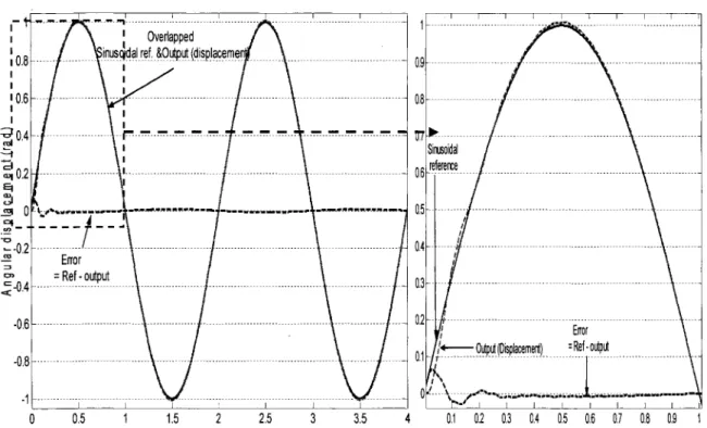
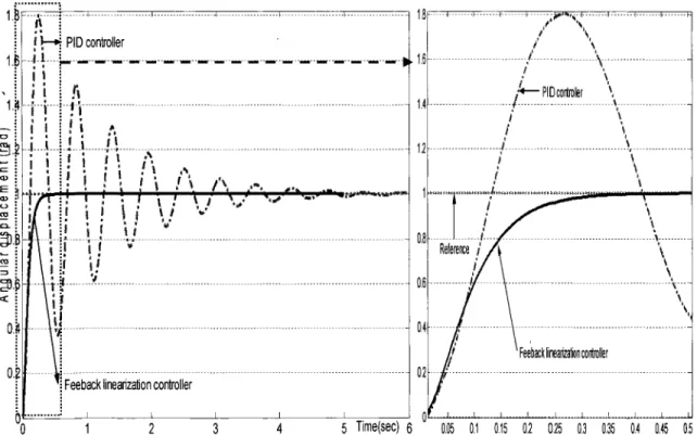
Figure 15 Unit step response of angular displacement by PID controller applied to linearized closed-loop system ... .45

Figure 16 Sinusoïdal response of angular displacement by PID controller applied to linearized closed-loop system ... .46

Figure 17 Comparison between variable with dimension and dimensionless variable as a controlled variable used for the feedback control system ... 47

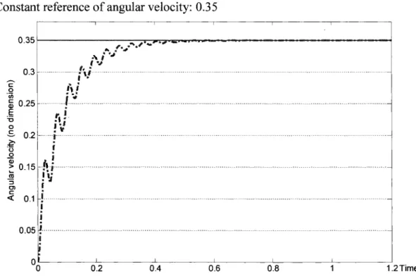
Figure 18 Constant response of dimensionless angular velocity by PID controller applied to linearized closed-loop system ... .48

Figure 19 Superposition of each response ... .49

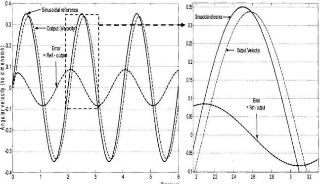
Figure 20 Sinusoïdal response of dimensionless angular velocity by PID controller applied to linearized closed-loop system ... 50 Figure 21 Constant response of dimensionless load pressure difference by PID

(14)

Figure 22 Sinusoïdal response of dimensionless load pressure difference by PID

controller applied to linearized closed-loop system ... 52

Figure 23 PID Controller in Nonlinear system ... 53

Figure 24 Unit step response of angular displacement by PID controller applied to nonlinear closed-loop system ... 54

Figure 25 Sinusoïdal response of angular displacement by PID controller applied to nonlinear closed-loop system ... 55

Figure 26 Constant response of dimensionless angular velocity by PID controller applied to nonlinear closed-loop system ... 56

Figure 27 Sinusoïdal response of dimensionless angular velocity by PID controller applied to nonlinear closed-loop system ... 57

Figure 28 Constant response of dimensionless load pressure difference by PID controller applied to nonlinear closed-loop system ... 58

Figure 29 Sinusoïdal response of dimensionless load pressure difference by PID controller applied to nonlinear closed-loop system ... 59

Figure 30 Design offeedback linearizable system ... 79

Figure 31 Comparison between feedback linearization based controller and PID controller for angular displacement control ... 81

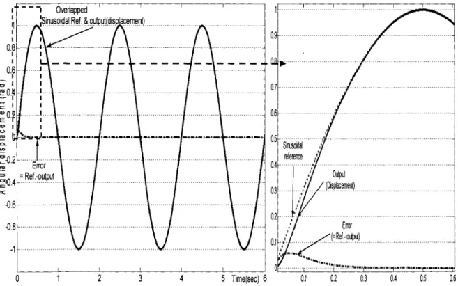
Figure 32 Sinusoïdal response of feedback linearization based controller for angular displacement control ... 82

Figure 33 Comparison between feedback linearization based controller and PID controller for angular displacement control.. ... 83

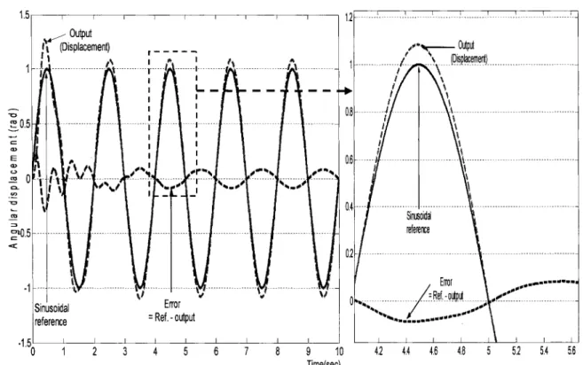
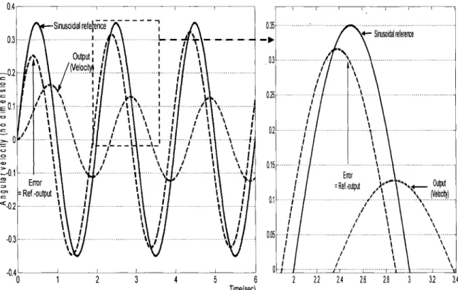
Figure 34 Sinusoïdal response offeedback linearization based controller for angular velocity ... 84

Figure 35 Comparison between feedback linearization based controller and PID controller for angular velocity control ... 85

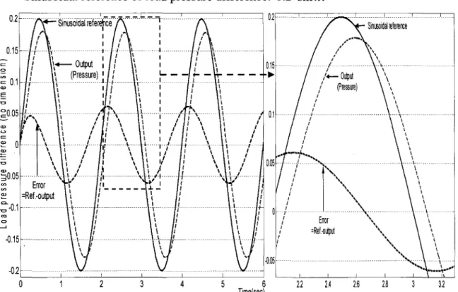
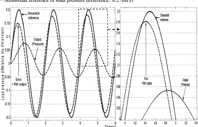
Figure 36 Sinusoïdal response of feedback linearization based controller for load pressure control ... : ... 86

Figure 37 Comparison between feedback linearization based controller and PID controller for load pressure control.. ... 87

Figure 38 Composition ofLITP test hench ... 91

Figure 39 RT-LAB HIL box and I/0 interface cards ... 92

(15)

Figure 41 Sensors used for real-time experiment.. ... 94

Figure 42 Simulink model separated into subsystems ... 95

Figure 43 SM_EH subsystem ... 96

Figure 44 SS_Feedback subsystem ... 98

Figure 4 5 SC_ U serinterface subsystem ... 1 00 Figure 46 RT-LAB main control console ... lOI Figure 4 7 Automatically launched visualization ... 1 02 Figure 48 Schematic of Open-loop real-time simulation for model validation ... 1 04 Figure 49 Comparison of angular displacement between mathematical model and real hydraulic system ... 1 05 Figure 50 Comparison of angular velocity between mathematical model and real hydraulic system ... 1 06 Figure 51 · Comparison of load pressure difference between mathematical model and real hydraulic system ... 1 07 Figure 52 Comparison ofreal-time simulation results between feedback linearization based controller and PID controller (Case 1-1) ... 11 0 Figure 53 Error comparison of feedback linearization based controller and PID controller (Case 1-1) ... 111

Figure 54 Comparison of control signais between the two controllers (Case 1-1) ... 112

Figure 55 Comparison ofreal-time simulation results between feedback linearization based controller and PID controller (Case 1-2) ... 113

Figure 56 Error comparison of feedback linearization based controller and PID controller (Case 1-2) ... 114

Figure 57 Comparison of real-time simulation results between feedback linearization based controller and PID controller (Case 1-3) ... 115

Figure 58 Error comparison of feedback linearization based controller and PID controller (Case 1-3) ... 116

(16)

Figure 61 Comparison of real-time simulation results between feedback

linearization based controller and PID controller (Case 2-1) ... 119 Figure 62 Error comparison of feedback linearization based controller and PID

controller (Case 2-1) ... 120 Figure 63 Comparison of control signais between the two controllers (Case 2-1) ... 121 Figure 64 Comparison ofreal-time simulation results between feedback

controller (Case 2-2) ... 123 Figure 66 Comparison ofreal-time simulation results between feedback

controller (Case 3-1) ... 127 Figure 70 Comparison of control signais between the two controllers (Case 3-1) ... 128 Figure 71 Comparison ofreal-time simulation results between feedback

linearization based controller and PID controller (Case 3-3) ... 131 Figure 74 Error comparison offeedback linearization based controller and PID

(17)

Avmax Maximum servo-valve opening area, m2

B Viscous damping coefficient, N ·rn· s

Cd Flow discharge coefficient

C,rn Intemalleakage coefficient, (rn 3/ s) 1 (N/m 2)

Cern Extemalleakage coefficient, (m3/s)/(N/m2)

CL Leakage coefficient, (m3/s)/(N/m2)

D rn Volumetrie displacement, m3/rad 1 Servo-valve input current, mA

1 max Maximum servo-valve input current, mA J Inertia load, N ·rn· s2

Ka Servo-valve amplifier gain, V/mA

Kv Servo-valve area constant, m2/m

Kx Servo-valve torque motor constant, mimA

~, 2 Pressures in actuator chambers, N/m2

~" Load pressure difference, N/m2

P, Supply pressure, N/m2

QI, 2 Flow rate in/out of actuator, m3/s

QL

Load flow, m3/s

Q,

Maximum supply flow, m3/s TL Actuator load torque, N · rn

(18)

e

Angular displacement, rad OJ Angular velocity, rad/s

OJh Hydraulic natural frequency, rad/s

OJmax Maximum angular velocity, rad/s

p

_{Fluid bulk modulus, N/m}2

p _{Fluid mass density, Kg/m}3

Tv Servo-valve time constant, s

Dimensionless Quantities

c,m Internalleakage coefficient

cern Externalleakage coefficient

CL Leakage load factor

i Servo-valve input current

P1,2 Pressures in actuator chambers

PL Load pressure difference

ql, 2 Flow rate in/out of actuator

qL Load flow

fL Load torque factor

xv Servo-valve opening area

a

Inertia load factor

r

Viscous load factor rjJ Angular velocity

(19)

• Problem statement and objective of research

Hydraulic systems play an indispensable role in motion and force actuation in several fields of application, due to advantages like high power, fast dynamic response and high robustness.

However, in spite of these merits, hydraulic systems have intrinsic control problems. In other words, hydraulic systems include nonlinearities resulting from flow dynamics, as well as hysteresis, friction and leakage, which make the modeling of these systems challenging. We include sorne of the se effects in our mode ling for control system design.

Due to the nonlinear nature of these systems, traditional linear methods like PID control have limitations in achieving high precision control of displacement, velocity and force. To overcome these limitations, we formulate an approach based on nonlinear theory.

Among the nonlinear strategies, the technique of feedback linearization is a viable approach to address problems induced by a certain class of system nonlinearities, by transforming a nonlinear system into an equivalent linear system by canceling out nonlinear terms.

In our study, the principal objective is to develop theoretical algorithms for angular displacement, angular velocity and pressure control of a rotational hydraulic drive with this nonlinear control technique. At the same time, our project will achieve the specifie objectives of:

(20)

• Development of control algorithms (i.e., PID controller and feedback linearization based controller) using the mathematical model that we develop

• Implementation of the control algorithms on a test bench, and comparison of the performance of each control algorithm

• Methodology

In this study, the sequence and method are as follows:

1. Description of the electro-hydraulic control system

The plant essentially consists of two electro-hydraulic servo-valves, one controlling the motion of the hydraulic motor and the other controlling the load torque of system. The oil is retumed through the servo-valve to the oil tank at atmospheric pressure.

2. Development of a mathematical model of the electro-hydraulic system (i.e., a fourth order state space model) to represent the system dynamics.

3. Design of a PID controller based on a linearized model of our nonlinear system and application of Ziegler-Nichols tuning rules. This designed PID controller will be applied to both the linearized and nonlinear system for simulation. The closed-loop simulation using unit step and sinusoïdal inputs will be performed in MATLAB/ Simulink. The closed-loop simulation results will provide insight into the performance limitations of PID control when it is applied to the nonlinear system.

4. Development of controllers for angular displacement, angular velocity and load pressure control of the nonlinear system based on the nonlinear control-design technique of feedback linearization. To evaluate its performance and compare it with the performance of PID controller, each controller will be tested in a

(21)

closed-loop simulation using the nonlinear plant model. MATLAB/Simulink will be used to perform these simulations.

5. Real-time simulation for experimental testing of each control algorithm (i.e., PID control and feedback linearization based control) proposed above will be conducted on a test bench of LITP (Laboratoire d'intégration des technologies de production). The work in this step includes a performance comparison between each feedback linearization based controller and the corresponding PID controller.

The key steps in the procedures outlined above are the performance comparisons of each controller through the simulation and experiment in Steps 4 and 5. Using these comparisons, we show that the feedback linearization based control strategy provides stable and accurate tracking performance for angular displacement, velocity and load pressure control of the nonlinear rotational hydraulic drive, and also overcomes the performance limitations of PID control.

• Organization of thesis

This thesis is organized in four parts.

In the first chapter, we present a comprehensive literature review, in which we will describe the typical features of electro-hydraulic servo-systems, the need for nonlinear theory and outline the approach for our research.

In the second chapter, we analyze the servo-system through modeling and describe the electro-hydraulic test bench used in our experiments.

In the third chapter, we perform a linearization based analysis of the system with respect to each output (i.e., angular displacement, angular velocity and load pressure difference)

(22)

using open-loop simulation in MATLAB/Simulink. We also describe the procedure to tune a PID controller using the Ziegler-Nichols method and then proceed to review feedback linearization theory for controller design. Finally, the comparative results of the tracking performance of each controller applied to the nonlinear system are analyzed using closed-loop simulation in MATLAB/Simulink.

In the fourth chapter, the comparative analysis of the performance of each controller is conducted on a test hench of LITP. We conclude by pro vi ding an overall assessment of our nonlinear control strategy.

(23)

LITERA TURE REVIEW

This chapter will first briefly describe the importance of electro-hydraulic servo-systems in modem industry, as well as the servo-system' s unique characteristics from the perspective of control. Secondly, through a comprehensive literature review, we will describe the approach to develop control algorithms for displacement, velocity and differentiai pressure of electro-hydraulic servo-systems based on our understanding of the typical features of these systems.

1.1 Advantages and disadvantages of Electro-hydraulic servo-system

There are many applications of Electro-hydraulic servo-system (EHSS) in several industries, for example, the automotive, aerospace and industrial automation industries, where large forces and torque are required along with fast dynamic response. The reasons why electro-hydraulic systems play an essential role in modem industrial applications are principally based on specifie features of these systems ( e.g., a high power/mass ratio, fast response, high stiffness and load capability). To use these advantages of hydraulic systems and to meet current industrial requirements (i.e., robust control with high accuracy and fast response ), control design for EHSS has become an active research area. However, the traditional approaches have limitations due to certain inherent characteristics of EHSS.

First, hydraulic systems include nonlinear elements that are difficult to model. Second, nonlinearities and parameter variations result in relatively complex plant behavior. Because of the inherently nonlinear nature of hydraulic systems, traditional linear control approaches cannot properly address the system's dynamics and thus have

(24)

limitations in terms of closed-loop performance. Therefore, the focus of our research is to apply a nonlinear control design technique to enhance controller performance.

1.2 Hydraulic drive control approaches

Although the control of a nonlinear system's outputs could be achieved through a general linearization, its control performance is only valid in the vicinity of the equilibrium operating point around which the system's equations are linearized. Thus, diverse approaches appropriate for nonlinear hydraulic systems have been introduced to go beyond traditionallinear methods.

Among them, the Variable Structure Control (VSC) technique deals with nonlinear systems through a fast switching control. It forces the original nonlinear system to behave as a stable linear one and achieves accurate servo tracking and consistent performance. But, despite the use of methods such as the reaching law [1] and sliding mode control [2], the discontinuity in switching control of most traditional VSC techniques results in a chattering effect, which may excite undesirable high-frequency dynamics.

The Perturbation Observer based nonlinear control [3] is another method for force control. With this proposed observer, accuracy for force control can be achieved, but it does not require position and velocity feedback. This approach is not suitable for displacement and velocity control. However, it provides a low-cost option for force control, since it does not require displacement and velocity sensors.

In order to address the discontinuity of the system at certain operational boundaries, a force-dependent gain-schedule model and Linear Parameter Varying (LPV) approach are introduced in [ 4] for velocity and force control. While satisfactory force control can be

(25)

achieved using this method, overshoot problems due to dead time are observed for velocity control.

Recently, many approaches have been introduced using Lyapunov functions. The Lyapunov based approach by Liu and Alleyne [5] is focused on reducing parameter uncertainties for force and pressure tracking. Another method based on Lyapunov function analysis, Backstepping Control, is a very robust method which guarantees system stability as well as high output tracking performance. The studies in [6], [7] and [8] describe representative applications of this method.

The main idea of backstepping is to transform the nonlinear system into a chain of integrators, and to construct a candidate Lyapunov function in terms of the error (i.e., difference between a state variable and its desired value). The control signal for the system is calculated by ensuring that the time derivative of the Lyapunov function is negative definite. Thus, the system is made globally asymptotically stable and asymptotic tracking is ensured. The flexibility for design is an important advantage of backstepping, as it makes good use ofuseful non-linearities.

Reference [7] provides an idea of the procedure for a system's stabilization through backstepping. If internai states that are not directly related to the controlled outputs are stable, we can exclude them from the main procedure for stabilizing a system. This idea can also be applied and be very helpful to our approach using feedback linearization.

However, one major weakness of backstepping is the many complicated procedures required to find the Lyapunov function of the whole system and the system's control signal. Therefore, a great deal of time and the attention during each step is necessary. This is especially so for high-order systems. Moreover, because the method can lead to a relatively large number of control parameters to stabilize the system, the determination of appropriate control parameter values that meet physical constraints such as actuator

(26)

performance limits can be challenging. Due to these drawbacks of the backstepping approach, we adopt feedback linearization theory, which is better suited to our study.

The methods outlined here have their own strengths and weakness, but they ali demonstrate that the application of nonlinear techniques is required for obtaining high performance control ofhydraulic systems.

1.3 Feedback linearization approach

The feedback linearization approach incorporates auxiliary measurements of sorne system states, which are used in the inverse model for canceling the nonlinearities. In our case, measurements of the load's position, velocity and pressure are required, and since sensors for these variables have been installed in the system, we are able to apply this method. Feedback linearization is also a theoretically rigorous method, utilizing a linearizing control law and state transformation, which transform the open-loop nonlinear system into a linear system in the closed-loop. The ability to use linear control design techniques after transforming the system is one of the advantages of using feedback linearization for control of nonlinear systems.

However, feedback linearization requires sorne limited conditions to be satisfied by the original nonlinear system. Specifically, the internai dynamics of the system described using a special state transformation need to be stable for the system to be fully linearized by the feedback law. Our electro-hydraulic servo-system satisfies the condition of being feedback linearizable for displacement, velocity and pressure control.

Studies in [ 6] and [9] for controlling velocity of a servo-system are good examples of the application of feedback linearization, but these studies only consider the case of a positive ramp output reference. In our study, we will diversify the types of output reference ( e.g., step and sinusoïdal input with various frequency and amplitude).

(27)

Noting the strengths and limitations of the various methods described above, we propose the study of feedback linearization theory for control of a nonlinear hydraulic system and provide a performance comparison with the classicallinear method, PID control.

1.4 Modeling and experimental setup

The first step of modeling prior to the experiment is to define the servo-system by its physical parameters and values. We base our modeling approach on that of [10] and [11], as the rotational hydraulic drive and experimental equipment used in their studies are identical to ours.

The key components of our servo-system are two servo-valves, of which one valve is for goveming the motor of the hydraulics drive and the other is for controlling the load torque or resistance. These servo-valves are driven by the control signal generated from the controller designed in our research and a constant arbitrary load command signal. Detailed information regarding these servo-valves will be provided in section 2.1 and 4.2.

For developing a model to describe the system's characteristics, we use a 4th order

nonlinear state space model. The most conspicuous feature in our state space model is that with the exception of angular displacement, other variables, like angular velocity, pressure and servo-valve opening area, are non-dimensionalized. By dividing each variable by its own maximum value, we make all variables dimensionless, and thus reduce numerical errors in the simulation results. A detailed explanation on dimensionless variables follows in section 2.2 ..

Another point of interest related to modeling is the application of the sigmoid function utilized in [8]. In the state space equation for load pressure difference and the control signal equation obtained by feedback linearization, we replace the sign function with a

(28)

sigmoid function, to overcome the Issues caused by the discontinuity and nondifferentiability of the sign function.

Althoug~ we follow the definition of parameters and use sorne of the values employed in [10], which describes the same electro-hydraulic system, other values are different from tho se in [ 1 0] because of different experimental conditions. We also use certain mathematical relationships between parameters to obtain precise parameter values instead ofthe approximated values utilized in [10].

1.5 Simulation and real-time control

As described in the methodology section, the comparison of simulation results between two controllers (i.e., PID and feedback linearization based controller) has significant meaning. Through this exercise, we can show the limited performance of PID control, which is widely utilized for industrial applications, and the excellent tracking ability of a controller designed by feedback linearization, a viable alternative that addresses the nonlinearities of the hydraulic system.

As comparative case studies, two types of simulation are used in our research. They include a fixed-step simulation in MATLAB/ Simulink and a real-time simulation on a test bench ofLITP using a commercial real-time system, i.e., RT-LAB.

As presented in [12, 13] and [13], RT-LAB has been used wide for industrial applications (e.g., robot, engine control systems and etc.) because it has severa} features:

• First, it allows us to execute real-time simulations based on compatibility with MATLAB/Simulink. Therefore, it provides a very convenient environment to design models and run real-time simulations of these models without special leaming and training for specifie software.

(29)

• Second, it provides a graphical user interface that allows us to check the simulation results synchronously.

• Third, during the simulation, we can edit our model design and change parameter values without having to modify C code.

The physical configuration of the RT-LAB system is comprised of a host computer and a real-time target. Using RT-LAB software on the host computer, we design the model for real-time simulation, and control the execution of the simulation on the real-time target. The target executes the real-time code, reads sensor data, generates analog signais that drive the servo-valves and also plays the role of linking the host computer from which we operate the controller, to the hydraulic system.

Execution ofRT-LAB real-time simulation models requires the following six steps:

• Creation of Simulink based model for real-time simulation

• Grouping the created model into subsystems (Master, slave and console subsystem) • Separation of the madel groups into sub-models and compilation of the models using

the compile option in the RT-LAB Main Control console

• Loading the executable file by using the load option in the RT-LAB Main Control console

• Execution of real-time simulation

(30)

In this chapter, we describe the main components of the electro-hydraulic system and develop a mathematical model (i.e., state space model) representing the system dynamics. We also exp lain the linearization of the state equations about an equilibrium point from which we create a Simulink model of the linearized system for simulation, and design a PID controller.

2.1 Setup of Electro-Hydraulic System

The electro-hydraulic system for this research is shown in Figure 1. A DC electric motor drives the pump, which induces oil from the oil tank to be delivered to each component of system. The oil is used for the operation of the hydraulic actuator and is returned through the servo-valve to the oil tank at atmospheric pressure. An accumulator and a relief valve are used to maintain a constant pressure supply from the output of the pump. The electro-hydraulic system essentially consists of two servo-valves which control the movement of the hydraulic rotary actuator and the load torque of the system respectively. These servo-valves are operated by signais generated by the real-time target. Additional explanations regarding the operation of the servo-valves are provided in Chapter 4.

(31)

(32)

2.2 Modeling of Electro-Hydraulic System

The modeling of the servo-system is based on the set-up shown in Figure 1 and

equations from reference [1 0]. As discussed briefly in chapter 1, the introduction of

several dimensionless variables (i.e., angular velocity, load pressure difference and servo-valve opening area except angular displacement) is needed in the mathematical description for modeling. These dimensionless variables can be obtained by dividing each variable by its own maximum value. Applying them reduces numerical errors during closed-loop simulation. Non-dimensionalizing the variables ensures that they are all in the same numerical range (i.e., 0 <range < 1 ).

In this section, we develop a mathematical model (i.e., state space model) with dimensionless variables, which describe the dynamics of our hydraulic system.

2.2.1 Servo-valve opening area and input command variables

All terms used for our mode ling are defined in the nomenclature of this thesis.

For the input command required for simulation, a dimensionless current to the servo-valve is defined as follows:

(33)

Dividing bath sides of this equation by Kx · Kv ·]max(= Avmax), we arrive at an equation presenting the relationship between the dimensionless servo-valve opening area and input command variable,

(2.1)

2.2.2 Load pressure difference variable

First, we need to define the dimensionless load pressure difference between the servomotor chamber pressures.

By definition,

R ft2

A =A-A

vJn-e

A=;, A.2=-p

s s

(2.2)

From reference [10], as well as the assumption that the servo-valve is critically centered, and the orifices are matched and symmetrical, we define the dimensionless flow rate in each actuator chamber as

(2.3)

(34)

Ifthe intemalleakage inside the servo-valve can be neglected, we can assume q₁

=

q₂at steady-state. Because of the fact that servo-valves are matched and symmetric, this assumption can be applied in our model. Moreover, if the extemal leakage of the servomotor can also be neglected, we are able to set q₁

=

q₂even in the transient state. Such a condition is usually considered true, because the extemal leakage is practically negligible.

Therefore, using equations of (2.3) and (2.4), and the assumption, q₁= q_{2 ,} it follows that

(2.5)

Using (2.2) and (2.5), we obtain

(2.6)

Substituting the result of (2.6) into (2.3) and (2.4) yields

Jix

~1-

PL

v 2 if xv> 0

ql

=

Jix

~1+

PI" _xv<₀

(35)

JixJl-pL

v

2

if xv> 0

q2

=

Jix

JI+

PI, _xv_<0

v

2

Therefore,

or, for ali conditions (i.e., positive and negative) of xv

qL =xv 1-PL

(FI)

(2.7)

=

xv~l-

Péign(xJ

From [10], the fluid dynamic equation in each actuator chamber can be expressed as follows.

For the first chamber:

or,

v

df1

- - =

_fJ

Q -

D OJ-C (P. - P)- C P.

(36)

Re-arranging this equation, we obtain

(2.8)

For the second cham ber:

U sing the same arrangement,

(2.9)

Next, from equations (2.2), (2.3), (2.4), (2.7), (2.8) and (2.9), it follows that

li]JL ~ CL

-=a(J) (q - --]J)

lit h L a L (2.1 0)

li]JL

=

a(J) (x

~1-

n sign(x ) -"'-cL n )

(37)

2.2.3 Angular velocity variable

The torque-acceleration relationship of the actuator is given by [1 0]. Neglecting the frictional torque, the relationship is

dm

J -_dt

=

D (P. -P )-Bm-1',

m 1 2 L

By dividing the above equation by J · OJmax, we obtain

(2.12)

From equations (2.2) and (2.12), the dimensionless angular velocity is given by

drjJ OJh

- = - ( p -rr/J-t)

dt Œ L L

(2.13)

2.2.4 Sigmoid fonction

(38)

EEJ

sign function sigmoid function

Figure 2 Comparison between sign and sigmoid function

We replace it with a sigmoid function, defined as

1 -e -ax

sigm(x)

=

_

1+e ax

(2.14)

From equation (2.14 ), we note that the sigmoid function is a continuously differentiable function, which has the following properties,

{

1 if ax ~oo

sigm(x)

=

0 if x = 0

-1 if ax ~ -oo

where a> 0 (2.15)

Its derivative is given by

dsigm(x)

=

-dx (1 + e-ax)2 (2.16)

Based on equations (2.15) and (2.16), we can plot the characteristic of the sigmoid function with the following graph,

(39)

yU 2 1.5 + a:o0.1 2 2.5 -1.5 -2

Figure 3 Graph of sigmoid function according to the variation of 'a' value

Here, we arbitrarily choose a=700 as a slope factor in order to approximate the sign function by the sigmoid function for simulation and experiment.

2.2.5 State Space Model

A state space model represents a physical system as n first order coupled differentiai equations. This form is better suited for computer simulation than an nth order input-output differentiai equation and is an effective way to analyze the system's nonlinearities. These merits are the main reasons for a state space model to be chosen as a mathematical model to describe the dynamics of our system.

(40)

Here, we express our system usmg a state space model with the four first order differentiai equations derived earlier and the sigmoid function.

For the state space model, we set x1

=

B, x2

=

rjJ, x3 =pL, x4

=

xv as state variables.

First, by rearranging equation (2.1 ), we obtain

Next, bythe applying equation (2.14) to (2.11) to replace the sign (xJ function, we get

From equation (2.13 ), it follows that

Finally, using the relation between x₁and x₂yields

dB

Where rjJ

=

_!!!__

=

_sjJ_ {Omax {Omax

(41)

From the four state equations above, we obtain the following state space model:

x

₁

x

=

X= 2

J;

(x" x2 , x3 , x 4 )

J;

(xl, x2, x3, x4 ,tL)

h

(xl, X2 ,x3, x4)

h

(xl, x2,x3, x4,i) Where

=

(J)h (J)h (J)h -r-x2 +-x3 --tL a a a

-a(J)hX2 - (J)hCL x3 + _a(J)hX4~1-_x3sigm(x4)

1 i

--x4

+-rv rv

For the state variable x

Xl=

e,

X2 = ___!!!___ = rjJ, X3 =

~

_{=pL, X4}=

~;ax

=Xv

(J)max 1 _S _"'v

For the command variable u

In (2.17), all variables except x1 are dimensionless.

2.3 Linearization

(2.17)

From the state space model (2.17), we note that this system has a nonlinear characteristic because of the square root factor in the equation for

x3.

Even though the system has a nonlinear characteristic, if the system opera tes around an equilibrium point, it is possible to approximate the nonlinear system by a linearized system.

In control engineering, the equilibrium point is typically considered to be a nominal operating point of the system. Therefore, the existence of the equilibrium point for the nonlinear system has a clear significance.

(42)

The first step in linearizing the nonlinear system is to determine its equilibrium point(s).

Let the equilibrium points be denoted by x₁₀, _{X20 , X30} and _{X40 •}

At the equilibrium point,

x

must be O.

From (2.17) OJh 01h OJh

-r-x2 +-x3 --tL

a

x

₁

x

-amhx2 -mhcLx3

+amhx

4 ~1-x

3 sigm(x

4 )

X=

x3

x

1 i

--x4

+-Tv Tv xl=xw Xz=Xzo X3=X3o x4=x40

0

0 0 0

From the equations above, we can easily find the equilibrium point of X (i.e., _{x 10 , x 20 , x 30}

XIO 0

Xzo 0

Xequilibrium point = Xo = =0

X3o 0

X4o 0

We now need the following Jacobian matrices in terms of x and u using Equation (2.17) to get a linearized system.

(43)

The Jacobian matrix in terms of x is given by

J=

x Where

a;;

_Oh

~

àx2

a;; a;;

~

àx2

a;; a;;

~

àx2

Oh Oh

~

àx2

=

-OJ c _{h L}

a;;

_Oh

àx} àx

₄

a;; a;;

àx} àx4

a;; a;;

àx} àx4

Oh Oh

àx} àx4

0 lümlX 0 0 0

-r-

lüh lüh 0

a

0 -amh -mhcL ao.Jh 0 0 0 1 Tv Xt=Xw X:l=Xzo X3=X3o x4=x40

aOJhX40 • X3o 2a. e -a•x40

bvr_o =X2o =X3o =x40 =0

l-e-a·x40

2 l x

-3o 1 + e -a•x40

(44)

The Jacobian matrix in terms of u is given by

a;; a;;

au] au2

0 0

a;; a;;

0 - OJh J _u=

au] au2

= a

aJ; aJ;

0 0

au] au2

1 0

ah ah

Tv

au] au2

Where

u

1 = i and

u2

= t,,

The mathematical model for the linearization of the nonlinear system m the neighborhood of the normal operating condition is then given by

U is the control signal; therefore, for the purpose of linearization, we can assume

U₀

=

0 (or 11U

=

U) .

Th us,

Xtmear

=

Jx x (X- Xo) + Ju x (U -Uo) =Jx X /1X +Ju X /1U

=

Jx xi1X +Ju xU

As X₀(Equilibrium point) = 0, it follows that

(2.18)

(45)

N ow, we can compactly express the linearized system using equations (2.18) and (2.19) as:

0 li) max 0 0 0 0

Ai

li)h li)h Llxl li)h

Ai 0

-r-

0 0

[:,]

M= a a Llx2 a 0 + 0 0 Ai -amh -Q)hCL amh _Llx3 3 Ai ₀ ₀ ₀ 1 Llx4 1 0

rv

=A·M+ B·U (2.20)

Next, we define a Y matrix to convert the dimensionless variables into variables with dimension in order to get actual outputs.

1 0 0 0 xl 0 li) max 0 0 x2 Y= 0 0 P, 0 x3 0 0 0 _~max x4 1 0 0 0 Llxl + XIO

0 li) max 0 0 Llx2 + X2o

= • : XIO = X2o = X30 = X 40 = 0 0 0 _~ 0 Llx3 + X3o 0 0 _{0 Av}max Llx4 + X4o 1 0 0 0 Llxl 0 li) max 0 0 Llx2 = 0 0

P,

0 Llx3 0 0 _{0 Av}max Llx4 =C·M+D·U (D=O) (2.21)

(46)

Finally, by replacing ali elements in the matrices above by their values listed in ANNEX 1, we obtain 0 173.45 0 0 0 0 0 -15.889 29.253 0 0 -29.253 A= B= 0 -657.45 -10.684 657.45 0 0 0 0 0 -100 100 0 1 0 0 0 0 0 0 173.45 0 0 0 0 C= 8.73xl06 D= 0 0 0 0 0 0 0 0 7.94 x 10-6 0 0

The se matrices A, B, C and D will be used to build a model of the linearized system for MATLAB/Simulink based simulation and to design a PID controller.

(47)

CONTROL ALGORITHMS AND VALIDATION

In this chapter, we compare our nonlinear system with the linearized system and describe the limitations of approximating a nonlinear system by a linear system. We also design a PID controller using the Ziegler-Nichols method and a feedback linearization based controller for the nonlinear system and verify the performance of each controller. 3.1 Open-loop simulation of nonlinear and linearized system

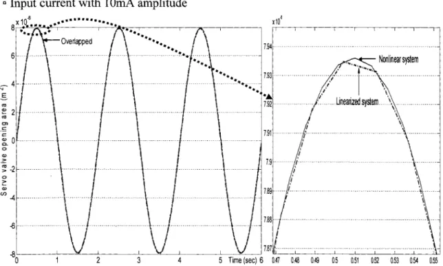
First, we intend to study the characteristics of angular displacement, angular velocity, load pressure difference and servo-valve opening area in the nonlinear system, using an open-loop simulation. Following that study, we want to compare the outputs of the nonlinear and linearized systems, and characterize how changes in the current input (i.e., high and low amplitude) impact the outputs of the two systems.

For the open-loop simulation study, the linear system matrices (i.e., A, B, C and D) and the state space model (2.17) were used for the linearized (Figure 4) and nonlinear system (Figure 5) respectively.

tl 1 - - - '

Input u2 (torque)

Figure 4 Linearized open-loop system

PreSSJre

(48)

Ail required simulations in this chapter were done using MA TLAB/Simulink. We used a sine wave for current input (u₁

=

i) that has two different amplitudes (low: lmA and high: lOmA) and the same frequency of n (rad/sec) . We also set the torque input ( u₂= tL ) to be 0 and the initial conditions of the nonlinear system were set to zero as in the case of the linearized system.

Sigmoid fuc

>-r----.[I}--+81

after x1 displacement

._______.8

ve\ocity '---< V \ 1 1 / a l p i + - - - _ . J

Figure 5 Nonlinear open-loop system

The following Figures provide a comparison of simulation results between the linearized and nonlinear systems in terms of each output variable.

(49)

• Simulation results • Angular displacement

c Input current with 1 OrnA amplitude

110,-~~~~.~ •• ,~~~-,~~~~.,r.,~~~~,-~~~~~,~~~--, ! \ - - - Linearized i \ / \ ... ., .f ... system .; \ . ... .. ... ..1 , 1 \ 1 ' 1 ... .l ... . .. L 100 90 ::0 ~ 80 ··+ ë 1 Q) 70 E ...

.,.

Q) (.) Cil 60 Ci. .!!l "0 <a 50 :; Cl c: 40 <( 30 20 10 0 o 1 2 3 4 5 6Time (sec)

Figure 6 Comparison of angular displacement at high amplitude input

c Input current with lmA amplitude

10 ::0 8 ~ ë Q) E Q) ₆ (.) Cil Ci. UJ 'ë _.... Cil :; 4 Cl c: <( 2 0 o 1 2 3 4 5 6Time (sec)

(50)

• Angular velocity

c Input current with 1 OrnA amplitude

150 100 û Q) .!!1 ""C ~

:5

₀ Qi > .... (Il :; -50 Cl c: <t: -100 -150 0

,.

..

...

i \ l \ ···~···\···

.,

.. ~Linearized system l ---·--··---· ~---\ \ \ 1 \ . . . \ ···.·r· ... l ... ···\ 1 \ 1 \ ! \J ~· ·~ 2 3 4 5 6Time (sec)

Figure 8 Comparison of angular velocity at high amplitude input

c Input current with 1 mA amplitude

15 û Q) .!!1 ""C ~ ~ 0 ₀ 0 Qi > .... ~ ::l -5 Cl c: <t: -10 -15 0 1 2 3 4 5 6Time (sec)

(51)

• Load pressure difference

o Input current with 1 OrnA amplitude 5 x 106

....

/ '.-Linearized system 4 ₁.- \ _•

.

\ 1 • 3 i -3 -- - - ~ -4

'·

\ '·

'

...

_·

1 ~

'

- - -

-,

'·

---\.-\ i

_....

-S0'---'---2'---__L3 _ _ _ _ _ 4'---__L5 _ _ _ _ __j6Time (sec)

Figure 10 Comparison of load pressure difference at high amplitude input

c Input current with 1mA amplitude

5x 10 5 N ..ê 2 -3 -4 2 3 4 5 6Time (sec;

(52)

• Servo-valve opening area

o Input current with 1 OrnA amplitude

ra ~ 2 ra C> .!':0 c: ~0 0 Q) z ~ -2 -80

·•···•·

2 3 x 10~ • •• • 7.93 .. ---~-!_,_., ____ _

..

7.92 .. 0.51 0.54 0.55

Figure 12 Comparison of servo-valve opening area at high amplitude input

o Input current with 1mA amplitude

.] 8 x 10 • • • • ••••••• -6 ..

..

_...

-- -- - ---··--·----••

...

7.95 .. " ' \ \ Unearized system \ Nonlinear system 8L__ _ _ _ _ __..._ _ __L__ _ _ _ J____,"'--__[ _ _ _ _ _ L - = - - - " " - - . - . J 7.8 . .... .. ... .... .. . . .. ... , .. - 0 1 2 3 4 5 Time (sec) 6 0.46 0.47 0.48 0.49 0.5 0.51 0.52 0.53 0.54 0.55 0.56

(53)

• Simulation results analysis

From the previous simulation results, the positive peak point value of each output is presented in the following tables.

Table I

Positive peak point value of angular displacement in relation to amplitude of current input

Linearized Difference rate

Current Nonlinear

Value oflinear.-value ofnonlinear. amplitude system system (=

value ofnonlinear. x lOO)

1 mA 10.94 rad 10.71 rad 2.14%

lOmA 109.4 rad 88.8 rad 23.19%

Increase rate

(From lmA 10 times 8.29 times

-to 10 mA)

Table II

Positive peak point value of angular velocity in relation to amplitude of current input

Difference rate

Current Linearized Nonlinear _{Value oflinear.-value ofnonlinear.}

amplitude system system (=

value of nonlinear. x lOO)

lmA 17.18 rad/s 16.73 rad/s 2.68%

lOmA 171.8 rad/s 131.6 radis 30.54%

Increase rate

(From lmA 10 times 7.86 times

(54)

Table III

Positive peak point value of load pressure difference in relation to amplitude of current input

Linearized Nonlinear Difference rate

Current _{Value of linear.-value of nonlinear.}

value of nonlinear. x lOO)

1 mA 4.82xl0 5 4.65xl05 3.22% N/m2 N/m2 lOmA 4.82xl0 6 3.65xl06 32.05% N/m2 N/m2 Increase rate 10 times 7.84 times (From lmA -to 10 mA) Table IV

Positive peak point value of servo-valve opening area in relation to amplitude of current input

Difference rate

Current Linearized Nonlinear _{Value oflinear.-value of nonlinear.}

value of nonlinear. x lOO) lmA 7.935 xl0-7 7.935 xl0-7 0% m2 m2 lOmA 7.934xl0-6 7.934xl0-6 0% m2 m2 Increase rate 10 times 10 times -(From lmA to 10 mA)

As noted from the figures, all outputs except angular displacement are symmetric with respect to the x axis in the open-loop nonlinear system. The asymmetry is explained as

(55)

follows: The velocity has a sine wave form ( e.g., A sin bt ), therefore the angular displacement is the integral of the angular velocity (i.e.,-A [cos bt

]~

=-A [ cos(bt) -1])

b

and is biased because by the constant term (i.e., A).

b

From the tables, ali outputs are directly affected by the change of current amplitude. Specifically, a factor of 10 increase of amplitude amplifies each output value by a factor of 7.84 to 10 times. As compared to the pattern of the linearized system, where the amplification factor (i.e., 10 times) of all outputs is equal to the change in amplitude (i.e., 1 0 times) of the input, the nonlinear system does not show such regularity in the relationship between output and input amplitude.

We also note that whereas the approximation of the nonlinear system by linearization is accurate for low amplitude (1 mA) current, the difference between each output value of the linearized and nonlinear systems is large at high amplitude (10 mA). (However, for the servo-valve opening area, there is no distinctive difference between the outputs of the two systems. This result can be explained by the fact that in contrast to the other outputs, the servo-valve opening has a linear relationship with the current as seen in equation (2.17).)

We are thus able to conclude that although the operation of system may be around equilibrium point, it is not possible to approximate the nonlinear system by the linear system unless the current input has small amplitude.

From these open-loop simulation results, we see that there are limitations to the use of linearization and traditional methods based on linearization are only effective in a narrow operating range, and thus, a nonlinear approach is required to provide high performance for the whole operating range.

(56)

3.2 PID controller

3.2.1 Introduction

Based on the mathematical model of the system that has been derived, various controllers can be designed to control the outputs of the rotational hydraulic system.

Among the various types of controllers, PID control is widely used due to its clear, simple structure, relatively good performance and low cost. Besicles, PID controllers can be easily modified, updated and auto tuned.

To design a PID controller to control our system, we choose the Ziegler-Nichols method, because it provides a convenient rule for controller tuning based on experimental response, and because it does not require a specifie process model or plant dynamic model.

In this section, we will apply the same PID controller obtained by the Ziegler Nichols method to both the linearized system and nonlinear system simultaneously and compare the results of simulation for each system to verify that the PID controller has limited control performance when applied to the nonlinear system, in terms of precision and response.

(57)

3.2.2 PID controller and Ziegler-Nichols method

Ziegler-Nichols tuning rules aim to limit maximum overshoot to 1 0~25%. Even though it does not guarantee extremely optimized tuning, it provides good control performance and has real usefulness when the plant dynamics are not known and analytical or graphical approaches to the design of controllers cannat be used. For example, the Ziegler-Nichols method does not need specifie characteristics of plant dynamics like the damping ratio and natural frequency of the system, since this method extracts the required information from experimental system response data. However, since we have a dynamic madel of the plant, we will use that model for the design of the PID controller.

The Ziegler- Nichols procedure is described briefly below:

Ziegler-Nichols rules (First and second method) are basically used to determine values of Kr (Proportional gain), ~ (Integral time) and Td (Derivative time ), which are the basic elements of a PID controller.

When we follow the second method, the first step IS to set ~

=

oo and Td

=

0 for designing a controller.

Next, applying Routh's stability criterion to the denominator of the closed-loop transfer function, we find Ker, the critical gain.

Finally, we use the experimentally determined tuning relationships based on OJ (Frequency of the sustained oscillation), ~r (Critical period) and Ker, to obtain the required parameters for a tuned PID controller.

(58)

We now present ali the steps to design a PID controller using the Ziegler-Nichols second method for angular displacement control in the linearized system.

Using the matrices obtained through linearization in Chapter 2 and the "ss2tf' function of MATLAB, we obtain a transfer function G(s) for the linearized system from current input to angular displacement output.

We first define new state matrices relating the current input and angular displacement output as follows:

Actes =A, Bdes = B(:,1)= 0 0 0 314.465

To reduce numerical errors in simulation, we take