i Université de Montréal
E¢ cient Estimation Using the Characteristic Function : Theory
and Applications with High Frequency Data
par
Rachidi KOTCHONI
Département de Sciences Économiques Faculté des Arts et des Sciences
Thèse présentée à la Faculté des Arts et des Sciences en vue de l’obtention du grade de
Philosophiae Doctor (Ph.D.) en Sciences Économiques
Mai, 2010
ii Université de Montréal
Faculté des Arts et des Sciences
Cette thèse intitulée :
E¢ cient Estimation Using the Characteristic Function : Theory and Applications with High Frequency Data
et présentée par :
Rachidi KOTCHONI
a été évaluée par un jury composé des personnes suivantes :
Marc HENRY Président-Rapporteur Marine CARRASCO Directeur de Recherche Benoit PERRON Membre du Jury
Russel DAVIDSON (McGill University) Examinateur Externe
Pierre DUCHESNE (D.M.S., U. de M)
Représentant du Doyen de la Faculté des Arts et Sciences
iii
Résumé de la thèse
Nous abordons deux sujets distincts dans cette thèse : l’estimation de la volatilité des prix d’actifs …nanciers à partir des données à haute fréquence, et l’estimation des paramétres d’un processus aléatoire à partir de sa fonction caractéristique.
Le chapitre 1 s’intéresse à l’estimation de la volatilité des prix d’actifs. Nous suppo-sons que les données à haute fréquence disponibles sont entachées de bruit de microstruc-ture. Les propriétés que l’on prête au bruit sont déterminantes dans le choix de l’estimateur de la volatilité. Dans ce chapitre, nous spéci…ons un nouveau modèle dynamique pour le bruit de microstructure qui intègre trois propriétés importantes : (i) le bruit peut être autocorrélé, (ii) le retard maximal au delà duquel l’autocorrélation est nulle peut être une fonction croissante de la fréquence journalière d’observations ; (iii) le bruit peut avoir une composante correlée avec le rendement e¢ cient. Cette dernière composante est alors dite endogène. Ce modèle se di¤érencie de ceux existant en ceci qu’il implique que l’autocor-rélation d’ordre 1 du bruit converge vers 1 lorsque la fréquence journalière d’observation tend vers l’in…ni.
Nous utilisons le cadre semi-paramétrique ainsi dé…ni pour dériver un nouvel estima-teur de la volatilité intégrée baptisée "estimaestima-teur shrinkage". Cet estimaestima-teur se présente sous la forme d’une combinaison linéaire optimale de deux estimateurs aux propriétés di¤érentes, l’optimalité étant dé…ni en termes de minimisation de la variance. Les simula-tions indiquent que l’estimateur shrinkage a une variance plus petite que le meilleur des deux estimateurs initiaux. Des estimateurs sont également proposés pour les paramètres du modèle de microstructure. Nous clôturons ce chapitre par une application empirique basée sur des actifs du Dow Jones Industrials. Les résultats indiquent qu’il est pertinent de tenir compte de la dépendance temporelle du bruit de microstructure dans le processus d’estimation de la volatilité.
Les chapitres 2, 3 et 4 s’inscrivent dans la littérature économétrique qui traite de la méthode des moments généralisés. En e¤et, on rencontre en …nance des modèles dont la fonction de vraisemblance n’est pas connue. On peut citer en guise d’exemple la loi stable ainsi que les modèles de di¤usion observés en temps discrets. Les méthodes d’inférence
iv basées sur la fonction caractéristique peuvent être envisagées dans ces cas. Typiquement, on spéci…e une condition de moment ht( ; 0) basée sur la di¤érence entre la fonction
caractéristique (conditionnelle) théorique et sa contrepartie empirique. Dans l’expression de cette condition de moment, 0 est la vraie valeur du paramètre d’intérêt et est la
variable de transformation de Fourier. Le dé…t ici est d’exploiter au mieux le continuum de conditions de moment ht( ; 0) ; 2 Rd pour atteindre la même e¢ cacité que le
maximum de vraisemblance.
Ce dé…t a été relevé par Carrasco et Florens (2000) qui ont proposé la procédure CGMM (continuum GMM). La fonction objectif que ces auteurs proposent est de la forme :
b
QT ( ; ) =
Z
Rd
K T1hT ( ; ) hT ( ; ) ( ) d
où ( )est une mesure …nie absolument continue sur Rd, hT ( ; 0)est le complexe
conju-gué de hT ( ; ) = T1
PT
t=1ht( ; ) et K 1
T est l’inverse régularisé de l’operateur de
cova-riance empirique associé à la fonction de moment ht( ; ). Le paramètre de régularisation
assure à la fois l’existence et la continuité de bQT ( ; ). Carrasco et Florens (2000) ont
montré que l’estimateur de 0 obtenu en minimisant bQT( ; ) est asymptotiquement aussi
e¢ cace que l’estimateur du maximum de vraisemblance si tend vers zéro lorsque la taille de l’échatillon T tend vers l’in…ni. La nature de la fonction objectif du CGMM sou-lève deux questions importantes. La première est celle de la calibration de en pratique, et la seconde est liée à la présence d’intégrales multiples dans l’expression de bQT ( ; ).
C’est à ces deux problématiques qu’essayent de répondent les trois derniers chapitres de la présente thèse.
Dans le chapitre 2, nous proposons une méthode de calibration de basée sur la minimisation de l’erreur quadratique moyenne (EQM) de l’estimateur. Nous suivons une approche similaire à celle de Newey et Smith (2004) pour calculer un développement d’ordre supérieur de l’EQM de l’estimateur CGMM de sorte à pouvoir examiner sa dé-pendance en en échantillon …ni. Nous proposons ensuite deux méthodes pour choisir en pratique. La première se base sur le développement de l’EQM, et la seconde se base sur des simulations Monte Carlo. Nous montrons que la méthode Monte Carlo délivre
v un estimateur convergent de optimal. Nos simulations con…rment la pertinence de la calibration de en pratique.
Le chapitre 3 essaye de vulgariser la théorie du chapitre 2 pour les modèles avec d 2. Nous commençons par passer en revue les propriétés de convergence et de norma-lité asymptotique de l’estimateur CGMM. Nous proposons ensuite des recettes numériques pour l’implémentation. En…n, nous conduisons des simulations Monte Carlo basée sur la loi stable. Ces simulations démontrent que le CGMM est une méthode …able d’inférence. En guise d’application empirique, nous estimons par CGMM un modèle de variance auto-régressif Gamma. Les résultats d’estimation con…rment un résultat bien connu en …nance : le rendement est positivement corrélé au risque espéré et négativement corrélé au choc sur la volatilité.
Lorsqu’on implémente le CGMM, une di¢ culté majeure réside dans l’évaluation numérique itérative des intégrales multiples présentes dans la fonction objectif. Les mé-thodes de quadrature sont en principe parmi les plus précises que l’on puisse utiliser dans le présent contexte. Malheureusement, le nombre de points de quadrature augmente expo-nentiellement en fonction de d. L’utilisation du CGMM devient pratiquement impossible dans les modèles multivariés et non markoviens où d 3. Dans le chapitre 4, nous propo-sons une procédure alternative baptisée "reéchantillonnage dans le domaine fréquentielle" qui consiste à fabriquer des échantillons univariés en prenant une combinaison linéaire des éléments du vecteur initial, les poids de la combinaison linéaire étant tirés aléatoirement dans un sous-espace normalisé de Rd. Chaque échantillon ainsi généré est utilisé pour
produire un estimateur du paramètre d’intérêt. L’estimateur …nal que nous proposons est une combinaison linéaire optimale de tous les estimateurs ainsi obtenus. Finalement, nous proposons une étude par simulation et une application empirique basées sur des modèles autorégressifs Gamma.
Dans l’ensemble, nous faisons une utilisation intensive du bootstrap, une technique selon laquelle les propriétés statistiques d’une distribution inconnue peuvent être estimées à partir d’un estimé de cette distribution. Nos résultats empiriques peuvent donc en principe être améliorés en faisant appel aux connaissances les plus récentes dans le domaine du bootstrap.
vi
Summary of the Thesis
In estimating the integrated volatility of …nancial assets using noisy high frequency data, the time series properties assumed for the microstructure noise determines the proper choice of the volatility estimator. In the …rst chapter of the current thesis, we propose a new model for the microstructure noise with three important features. First of all, our model assumes that the noise is L-dependent. Secondly, the memory lag L is allowed to increase with the sampling frequency. And thirdly, the noise may include an endogenous part, that is, a piece that is correlated with the latent returns. The main di¤erence between this microstructure model and existing ones is that it implies a …rst order autocorrelation that converges to 1 as the sampling frequency goes to in…nity.
We use this semi-parametric model to derive a new shrinkage estimator for the integrated volatility. The proposed estimator makes an optimal signal-to-noise trade-o¤ by combining a consistent estimators with an inconsistent one. Simulation results show that the shrinkage estimator behaves better than the best of the two combined ones. We also propose some estimators for the parameters of the noise model. An empirical study based on stocks listed in the Dow Jones Industrials shows the relevance of accounting for possible time dependence in the noise process.
Chapters 2, 3 and 4 pertain to the generalized method of moments based on the characteristic function. In fact, the likelihood functions of many …nancial econometrics models are not known in close form. For example, this is the case for the stable distribution and a discretely observed continuous time model. In these cases, one may estimate the parameter of interest 0 by specifying a moment condition ht( ; 0)based on the di¤erence
between the theoretical (conditional) characteristic function and its empirical counterpart, where 2 Rd is the Fourier transformation variable. The challenge is then to exploit
the whole continuum of moment conditions fht( ; 0) ; 2 Rpg to achieve the maximum
vii This problem has been solved in Carrasco and Florens (2000) who propose the CGMM procedure. The objective function of the CGMM is given by :
b
QT ( ; ) =
Z
Rd
K T1hT ( ; ) hT ( ; ) ( ) d
where ( )is an absolutely continuous …nite measure, hT ( ; )is the complex conjugate of
hT ( ; ) = T1
PT
t=1ht( ; )and K 1
T is the regularized inverse of the empirical covariance
operator associated with the moment function. The parameter ensures the existence as well as the continuity of bQT ( ; ). Carrasco and Florens (2000) have shown that the
estimator obtained by minimizing bQT ( ; ) is asymptotically as e¢ cient as the maximum
likelihood estimator provided that converges to zero as the sample size T goes to in…nity. However, the nature of the objective function bQT ( ; ) raises two important questions.
First of all, how do we select in practice ? And secondly, how do we implement the CGMM when the multiplicity of the integrals embedded in the objective-function d is large. These questions are tackled in the last three chapters of the thesis.
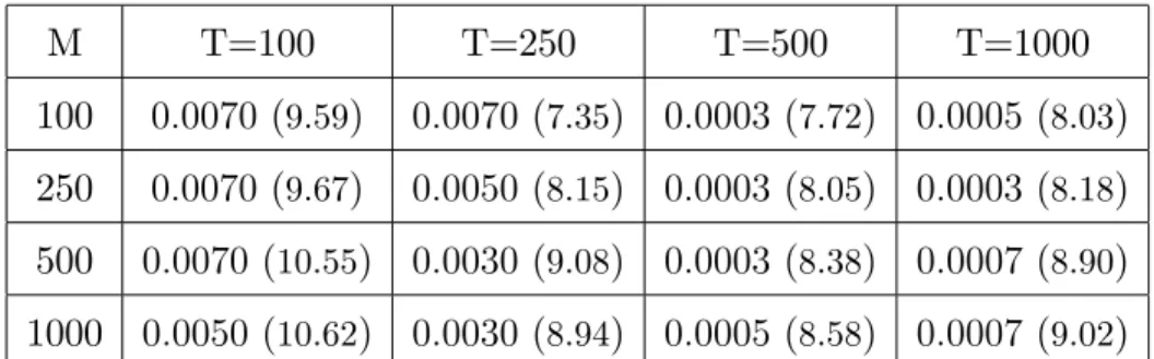
In Chapter 2, we propose to choose by minimizing the approximate mean square error (MSE) of the estimator. Following an approach similar to Newey and Smith (2004), we derive a higher-order expansion of the estimator from which we characterize the …nite sample dependence of the MSE on . We provide two data-driven methods for selecting the regularization parameter in practice. The …rst one relies on the higher-order expansion of the MSE whereas the second one uses only simulations. We show that our simulation technique delivers a consistent estimator of . Our Monte Carlo simulations con…rm the importance of the optimal selection of .
The goal of Chapter 3 is to illustrate how to e¢ ciently implement the CGMM for d 2. To start with, we review the consistency and asymptotic normality properties of the CGMM estimator. Next we suggest some numerical recipes for its implementation. Finally, we carry out a simulation study with the stable distribution that con…rms the accuracy of the CGMM as an inference method. An empirical application based on the autoregressive variance Gamma model led to a well-known conclusion : investors require
viii a positive premium for bearing the expected risk while a negative premium is attached to the unexpected risk.
In implementing the characteristic function based CGMM, a major di¢ culty lies in the evaluation of the multiple integrals embedded in the objective function. Numerical quadratures are among the most accurate methods that can be used in the present context. Unfortunately, the number of quadrature points grows exponentially with d. When the data generating process is Markov or dependent, the accurate implementation of the CGMM becomes roughly unfeasible when d 3. In Chapter 4, we propose a strategy that consists in creating univariate samples by taking a linear combination of the elements of the original vector process. The weights of the linear combinations are drawn from a normalized set of Rd. Each univariate index generated in this way is called a frequency domain bootstrap sample that can be used to compute an estimator of the parameter of interest. Finally, all the possible estimators obtained in this fashion can be aggregated to obtain the …nal estimator. The optimal aggregation rule is discussed in the paper. The overall method is illustrated by a simulation study and an empirical application based on autoregressive Gamma models.
This thesis makes an extensive use of the bootstrap, a technique according to which the statistical properties of an unknown distribution can be estimated from an estimate of that distribution. It is thus possible to improve our simulations and empirical results by using the state-of-the-art re…nements of the bootstrap methodology.
Contents
Sigles et Abréviations . . . 7
Dédicace . . . 8
Remerciements . . . 9
1 Shrinkage Realized Kernels 11 1.1 Introduction . . . 11
1.2 Motivating Shrinkage Estimators for the IV . . . 14
1.2.1 The E¢ cient Price and the Microstructure Noise . . . 14
1.2.2 Three Standard Estimators of the IV . . . 16
1.2.3 Discretization Error versus Microstructure Noise . . . 19
1.2.4 Asymptotic Theory . . . 22
1.3 A Semiparametric Model for the Microstructure Noise . . . 24
1.3.1 Assumptions . . . 25
1.3.2 Nested and Related Models . . . 26
1.3.3 Some Implications of the Model . . . 28
1.4 Properties of Three IV Estimators . . . 29
1.4.1 The Realized Volatility . . . 30
1.4.2 Hansen and Lunde (2006) . . . 32
1.4.3 Barndor¤-Nielsen, Hansen, Lunde and Shephard (2008a) . . . 34
1.5 Inference on the Microstructure Noise Parameters . . . 37
1.5.1 Estimation of the Correlogram . . . 37
1.5.2 Assessing the true values of L, and . . . 40
1.6 Shrinkage Realized Kernels . . . 41
1.7 Monte Carlo Evidence . . . 45
2
1.7.1 Simulation Design . . . 45
1.7.2 Simulation Results . . . 47
1.8 Empirical Application . . . 49
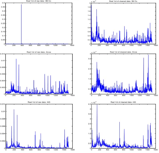
1.8.1 Data and Preprocessing . . . 49
1.8.2 Empirical Results . . . 50
1.9 Conclusion . . . 51
Bibliographie . . . 53
Appendices . . . 58
2 E¢ cient Estimation Using the Characteristic Function 77 2.1 Introduction . . . 77
2.2 Overview of the CF-based CGMM . . . 80
2.3 Stochastic expansion of the CGMM estimator . . . 85
2.4 Optimal selection of the regularization parameter . . . 87
2.4.1 Estimating the MSE using its higher order expansion . . . 89
2.4.2 Estimating the MSE by standard Monte Carlo . . . 90
2.4.3 Optimality of the data-driven selection of the regularization parameter 91 2.5 Monte Carlo Simulations . . . 93
2.5.1 The simulation design . . . 93
2.5.2 The simulation results . . . 94
2.6 Conclusion . . . 95
Bibliographie . . . 97
Appendices . . . 101
3 Applications of the Characteristic Function Based Continuum GMM in Finance 129 3.1 Introduction . . . 129
3.2 The CGMM: a Brief Theoretical Review . . . 131
3.2.1 The CGMM in the IID Case . . . 131
3.2.2 The CGMM with Dependent Data . . . 134
3.2.3 Basic Assumptions of the CGMM . . . 136
3
3.3.1 Computing the Objective Function by Quadrature Method . . . 137
3.3.2 Computing the Objective Function by Monte Carlo Integration . . . 140
3.3.3 Computing the Variance of the CGMM Estimator . . . 141
3.3.4 Data-driven Selection of the Regularization Parameter . . . 142
3.4 Estimating the Stable Distribution by CGMM: a Simulation Study . . . 144
3.4.1 Parametrizations of the Stable Distribution . . . 144
3.4.2 Simulating from the Stable Distribution . . . 147
3.4.3 Monte Carlo Experiments . . . 149
3.5 Fitting the Autoregressive Variance Gamma Model to Assets Returns . . . . 153
3.5.1 The Autoregressive Variance Gamma Model . . . 154
3.5.2 Simulating the ARVG model . . . 156
3.5.3 Estimating the ARVG Model from High Frequency Data . . . 156
3.5.4 Empirical Application . . . 159
3.6 Conclusions . . . 161
Bibliographie . . . 162
Appendices . . . 167
4 A Solution to the Curse of Dimensionality in the Continuum GMM 170 4.1 Introduction . . . 170
4.2 The General Framework . . . 174
4.2.1 The Objective functions . . . 174
4.2.2 The Assumptions . . . 176
4.3 Properties of the CGMM Estimators . . . 177
4.4 The Ideal FCGMM Estimator . . . 180
4.4.1 Consistency and Optimal Aggregating Measure . . . 181
4.4.2 Comparison with the Maximum Likelihood . . . 182
4.5 The Feasible Optimal FCGMM . . . 184
4.6 A Simulation Study . . . 187
4.6.1 The Autoregressive Factor Gamma Model . . . 188
4.6.2 Estimating the ARFG Model from Observed Returns . . . 190
4
4.7 An Empirical Application . . . 193
4.7.1 The Autoregressive Variance Gamma Model or Order p . . . 194
4.7.2 Estimation of the ARVG(p) Using High Frequency Data . . . 196
4.7.3 An Application with the Alcoa Index . . . 197
4.8 Conclusion . . . 199
Bibliographie . . . 201
Appendices . . . 203
List of Tables
Table 1.1: Part of the MSE due to discretization . . . 20
Table 1.2: Simulation with no Leverage e¤ect. . . 71
Table 1.3: Simulation with Leverage e¤ect. . . 72
Table 1.4: Estimated the correlogram of the noise (Simulated Data). . . 73
Table 1.5: Estimates of L, alpha and delta for twelve stocks listed in the DJI. . . . 74
Table 2.1: Estimation of the optimal regularisation parameter for di¤erent T and M. 95 Table 3.1: Simulation Results for the Stable Distribution with alpha=1.5 . . . 151
Table 3.2: Simulation Results for the Stable Distribution with alpha=1.95 . . . . 152
Table 3.3: Bootstrap statistics . . . 160
Table 4.1: Monte Carlo simulations results for the ARFG Model estimated by CGMM-FB . . . 193
Table 4.2: Summary of the Estimation Results . . . 198
List of Figures
Figure 1.1: The subsampling scheme . . . 30
Figure 1.2: Detecting Noise in the Data. . . 70
Figure 1.3: Preprocessing the data. . . 75
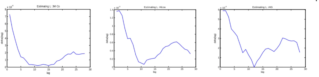
Figure 1.4: Estimation Results for 3M Co, Alcoa and AIG. . . 76
Figure 2.1: MSE of the CGMM estimator . . . 95
Figure 3.1: Choosing the optimal regularization parameter. . . 151
Figure 4.1: The mean square error of the CGMM-FB estimator . . . 193
Figure 4.2: Selecting the regularization parameter . . . 197
Figure 4.3: Estimated Autoregressive Roots for the Volatility . . . 198
Figure 4.4: Fitted Values for the Volatility . . . 199
7
Sigles et abréviations
ARCH : Autoregressive Conditional Heteroscedasticity ARFG : Autoregressive Factor Gamma
ARVG : Autoregressive Variance Gamma CF : Characteristic Function
CIR : Cox Ingersol and Ross
CGMM : Continuum Generalized Method of Moments ECF : Empirical Characteristic Function
GARCH : Generalized Autoregressive Conditional Heteroscedasticity GMM : Generalized Method of Moments
FB : Frequency domain Bootstrap
IID : Independent and Identically Distributed MSE : Mean Square Error
IV : Integrated Volatility RV : Realized Volatility
8 A mes parents, Alimatou Aboudou et Bio Séidou Kotchoni,
La ‡amme qu’ils ont allumé brûle encore, contre toutes les attentes. A ma tante, Salamatou Aboudou Touré,
9
Remerciements
Tout d’abord, je remercie une excellente directrice de recherche, Marine Carrasco, pour sa disponibilité et sa grande patience. Son support a été très déterminant dans la réussite de ce projet de thèse.
Ensuite, j’adresse un merci spécial à toutes les personnes qui, dans les moments de doutes, m’ont encouragé à continuer. Je citerais Gérard Gaudet, Prosper Dovonon et son épouse Olivia, Firmin Doko et son épouse Carole. Pour tout le soutien qu’ils m’ont apporté, je remercie toute ma famille et plus particulièrement mes parents Alimatou Aboudou et Séidou Kotchoni, mes frères et soeurs, mes oncles Toussaint Kegnidé, Michel Biaou ainsi que leurs épouses. C’est le lieu de mentionner ma gratitude à Chakirou Razaki dont la contribution à cette thèse date de bien avant le début de la thèse. A lui et à toute sa famille, je souhaite beaucoup de joie et de bonheur.
Pour la qualité de leurs conseils, suggestions ou soutiens, je remercie les professeurs Marcel Boyer, Benoit Perron, Marc Henry, Rui Castro, Sílvia Gonçalves. Je remercie tous les pro-fesseurs du Département des Sciences Économiques de l’Université de Montréal pour la qualité de leurs enseignements. Je rends hommage à Mme Larouche-Sidoti, Mme Lyne Racine, Mme Jocelyne Demers, Mme Josée Lafontaine et tout le personnel du CIREQ pour leur précieuse contribution dans la bonne marche du département.
J’éprouve une profonde gratitude envers les organismes qui m’ont apporté directement ou indirectement un soutien matériel et …nancier tout au long de ma formation: la Banque Lau-rentienne, le Centre Interuniversitaire de Recherche en Analyse des Organisations (CIRANO), le Centre Interuniversitaire de Recherche en Économie Quantitative (CIREQ), le Départe-ment des Sciences Économiques ainsi que la Faculté des Études Supérieures de l’Université de Montréal.
Pour toutes sortes de choses qu’il serait trop long d’énumérer ici, mes sincères remer-ciements vont également à mes amis Constant Lonkeng, son épouse Judith et sa …lle Abigael, Octave Keutiben et son épouse Sylvie, Bruno Feuno, Constantin Hèdiblè et son épouse Gra-cia, Clément Yélou et son épouse Jocelyne, Messan Agbaglah, Modeste Somé, Sali Sanou, Nerée Noumon, Cédric Okou, Bertrand Hounkannounon, Jonhson Kakeu, Anderson Wal-ter Nzabandora, Moudjib Moussiliou Coles et son épouse Semirath, sans oublier mes amis
10 Kenneth Tanimomo et Francis Biaou.
Aux nombreuses personnes que je ne cite pas et qui ont contribué à la réussite de ce projet de thèse de près ou de loin, j’adresse un merci qui vient du coeur.
Chapter 1
Shrinkage Realized Kernels
Note: Cet article rédigé en collaboration avec Marine Carrasco est actuellement sous évaluation pour publi-cation dans "Journal of Financial Econometrics"
Mots-Clés: Integrated Volatility, Method of Moment, Microstructure Noise, Realized Kernel, Shrinkage.
1.1
Introduction
Since the theoretical works by Jacod (1994), Jacod and Protter (1998) and Barndor¤-Nielsen and Shephard (2002), it is well established that the realized volatility (RV) is a consistent estimator of the integrated volatility (IV) when prices are observed without error (see for example Ait-Sahalia, Mykland and Zhang, 2005). However, it is commonly admitted that recorded stock prices are contaminated with pricing errors known in the literature as the "market microstructure noise" (henceforth "noise"). The causes of this noise are discussed for example in Stoll (1989, 2000) or Hasbrouck (1993,1996). In the words of Hasbrouck (1993), the pricing errors are mainly due to "... discreteness, inventory control, the non-information based component of the bid-ask spread, the transient component of the price response to a block trade, etc.". Its presence in measured prices causes the RV computed with very high frequency data to be a severely biased estimator of the IV.
Many approaches have been proposed in the literature to deal with this curse. One of them consists in choosing in an ad-hoc manner a moderate sampling frequency at which the
12 impact of the noise is su¢ ciently mitigated1. Zhou (1996) and Hansen and Lunde (2006)
proposed a bias correction approach while Bollen and Inder (2002) and Andreou and Ghy-sels (2002) advocated …ltering techniques. Under the assumption that the volatility of the high frequency returns are constant within the day, Ait-Sahalia, Mykland and Zhang (2005) derived a highly e¢ cient maximum likelihood estimator of the IV that is robust to both IID noise and distributional mispeci…cation. Zhang, Mykland, and Ait-Sahalia (2005) proposed another consistent estimator in the presence of IID noise which they called the two scale re-alized volatility. This estimator has been adapted in Ait-Sahalia, Mykland and Zhang (2006) to deal with dependent noise. Since then, other consistent estimators have become avail-able among which the realized kernels of Barndor¤-Nielsen, Hansen, Lunde and Shephard (2008a) and the pre-averaging estimator of Podolskij and Vetter (2006)2. An alternative line of research pursued by Corradi, Distaso and Swanson (2008) advocates the nonparametric estimation of the predictive density and con…dence intervals for the IV rather than focusing on point estimates.
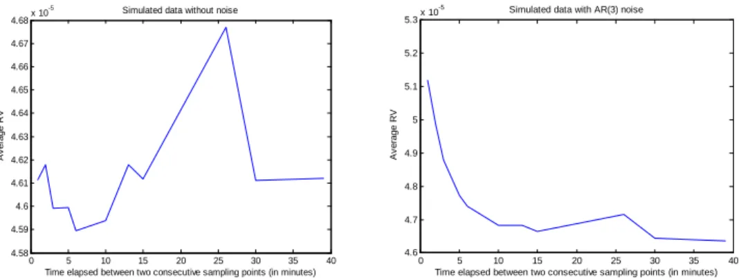
In a simulation study, Gatheral and Oomen (2007) showed that consistent estimators often perform poorly at the sampling frequencies commonly encountered in practice. One can explain this result by saying that an inconsistent estimator necessarily delivers its best performance at moderate frequency3 while a consistent estimator may require quite high
frequency data in order to perform well. It turns out from our simulations study of Section 8 that the conclusion of Gatheral and Oomen (2007) strongly depends on the size of the variance of the microstructure noise relative to the discretization error. In fact, the inconsistent estimator tends to perform better than the consistent one only when the variance of the microstructure noise is small. The main idea of the current paper is that even when the variance of the inconsistent estimator is higher, it can still be optimally combined with the consistent estimator to obtain a new one that performs better than both. The weight of the linear combination is selected in order to minimize the variance and the resulting estimator is called "shrinkage realized kernels".
However, a good estimator of the IV must be designed in accordance with the dependence
1See Andersen, Bollerslev, Diebold and Labys (2000); Andersen, Bollerslev, Diebold and Ebens (2001). 2See also Jacod, Li, Mykland, Podolskij and Vetter (2009).
13 properties of the noise. Awartani, Corradi and Distaso (2007) proposed an hypothesis test to assess the impact of certain features of the noise on realized measures. Hansen and Lunde (2006) construct a Haussman-type test to detect time dependence in the noise process. After applying their test to real data, they concluded that the noise process is time dependent, correlated with latent return, and possibly heteroscedastic4. More recently, Ubukata and Oya
(2009) proposed some procedures to test for dependence in the noise process in a bivariate framework with irregularly spaced and asynchronous data.
In this paper, we restrict our attention to regularly spaced univariate data and advocate a semi-parametric model for the noise. More precisely, we specify at the highest frequency a parsimonious relation between the microstructure noise on the one side, and the e¢ cient return and the latent volatility process on the other side. We assume a general and ‡exible type of noise that includes an independent endogenous part "s and an L-dependent exogenous part "s. Contrary to an AR(1) model with constant autoregressive root, the new model has
the implication that the correlation between two consecutive realizations of "t converges to
one as the frequency at which the prices are recorded goes to in…nity. This model captures the fact that two consecutive observations of "t become arbitrarily close in calendar time and
eventually coincide at the limit as the sampling frequency increases.
We derive the properties of common realized measures under the model and propose new unbiased estimators for the IV. One unbiased estimator uses the samples available at all days to estimate the IV of each day, while the second only uses within day data. The shrinkage realized kernels are …nally designed as the optimal linear combination of the standard realized kernels of Barndor¤-Nielsen and al. (2008a) with the unbiased within day estimator. We also propose a framework to estimate the exogenous noise parameters. Unfortunately, the endogeneity parameters are not identi…able.
We illustrate by simulation the good performance of the shrinkage realized kernels pro-posed estimator. An empirical application based on …fteen stocks listed in the Dow Jones Industrials shows strong evidences of correlation in the noise process and between the noise and the latent returns. Indeed, the empirical results suggest that the memory parameter L grows slower thanpm in general. It should be mentioned that this result is derived under
4Kalnina and Linton (2008) propose a consistent estimator in the presence of a noise that exhibits diurnal
14 the assumption that our model for the microstructure noise is true.
The rest of the paper is organized as follows. The next section motivates the use of shrinkage estimators for the IV when the noise is IID. In Section 3, we present our theoretical model in light of which we study the properties of three standard IV estimators in section 4. Inference procedures about the noise parameters are presented in section 5. In Section 6, we design the shrinkage realized kernels for the dependent noise case. Sections 7 and 8 present respectively a simulation study and an empirical application based on twelve stocks listed in the Dow Jones Industrials. Section 9 concludes. The mathematical proofs and the summaries of the results of Sections 7 and 8 are gathered in appendix.
1.2
Motivating Shrinkage Estimators for the IV
Basically, a shrinkage estimator is an optimal linear combination of several estimators. Here, optimal means that shrinkage estimator minimizes the mean square error (MSE). To motivate shrinkage estimators for the IV, we examine the contribution of the discretization error and the microstructure noise to the MSEs of three estimators. More precisely, we try to understand the trade-o¤s at play as one moves from a biased estimator to an unbiased estimator on the one hand, and from an unbiased estimator to a consistent estimator on the other hand.
To start with, we introduce some basic notation and concepts.
1.2.1
The E¢ cient Price and the Microstructure Noise
Let ps denote a latent (or e¢ cient) log-price of an asset and ps its observable counterpart.
Assume that the latent log-price obeys the following stochastic di¤erential equation:
dps = sdWs; p0 = 0 (1.1)
where Ws is a standard Brownian motion independent of s.
Keeping in mind that we are working with high frequency data, the omitted drift is proportional to ds which is negligible in front of the Op
p
ds volatility term. We assume that the volatility process f sg
T
15 are locally integrable with respect to the Lebesgue Measure5. Without loss of generality, we
condition all our analysis on the whole volatility path but the conditioning is removed from the notations for simplicity. Therefore, all deterministic transformations of the volatility process are treated as constant objects. In particular, the integrated volatilities IVt =
Rt t 1
2 sds;
t = 1; 2; 3; :::T are …xed parameters we aim to estimate. We will consider a sampling scheme where the unit period is normalized to one in calendar time.
It is maintained throughout the paper that there is neither jump nor leverage e¤ect in our model for the e¢ cient price. If jumps that are uncorrelated with all other randomness are added in the model, the estimators considered for the IV in the sequel are now designed for the quadratic variation6. If leverage e¤ect is assumed in (1.1), some of our results can
be derived with a few more technical complications. We will check the robustness of our conclusions to the presence of leverage e¤ect in simulation.
By de…nition, the noise equals us = ps ps; that is, the di¤erence between the observed
log-price and the e¢ cient log-price. Let rt denote the latent log-return at period t, and rt
its observable counterpart. Under the above conditions, the process frtg is a semimartingale
and we have: rt pt pt 1= rt + ut ut 1 (1.2) rt = Z t t 1 sdWsj f sgTs=0 N (0; IVt) (1.3)
Suppose that we have access to a large number m of intra-period returns rt;1; rt;2; :::; rt;m,
where t = 1; :::; T are the period labels, m is the number of recorded prices in each period and rt;j is the jth observed return during the period [t 1; t]. In the sequel, we sometimes
use the expression "record frequency" to refer to the frequency m at which the data has been recorded. The noise-contaminated (observed) and true realized volatility (latent) computed at frequency m are: RVt(m) = m X j=1 rt;j2 and RVt(m) = m X j=1 rt;j2 (1.4)
5See e.g Barndor¤-Nielsen, Graversen, Jacod and Shephard (2006).
6Separating the IV from the contribution of the jumps in the quadratic variation would then be the new
16 For simplicity, we assume that these observations are equidistant in calendar time. We have:
rt;j pt 1+j=m pt 1+(j 1)=m = Z t 1+j=m t 1+(j 1)=m sdWs rt;j = rt;j + ut;j ut;j 1 ut;j ut 1+j=m
Barndor¤-Nielsen and Shephard (2002) show that RVt(m) converges to IVt and derived
the asymptotic distribution:
RVt (m) IVt q 2 3 Pm j=1r 4 t;j ! N(0; 1)
as m goes to in…nity. Meddahi (2002) studied the …nite frequency behavior of the discretiza-tion error RVt(m) IVtwith a focus on the speci…c case where the true model belongs to the
Eigenfunction Stochastic Volatility family. Gonçalves and Meddahi (2009) proposed some bootstrap procedures as alternative inference tools to analyze the asymptotic behavior of realized measures. In both papers, no microstructure noise is assumed.
In the presence of microstructure noise, RVt (m) is no longer feasible. We review three
feasible estimators below.
1.2.2
Three Standard Estimators of the IV
In this subsection, we consider estimators cIVt of IVt such that:
c IVt= fr rt;j m j=1 + fr ;u rt;j; ut;j m j=1 + fu fut;jg m j=1 (1.5) with Ehfr rt;j m j=1 i = IVt (1.6) Ehfr ;u rt;j; ut;j m j=1 i = 0 (1.7) and fr ;u rt;j; 0 m j=1 = fu f0g m j=1 = 0 (1.8)
17 Below are three examples of estimators that can be decomposed as above.
Example 1 The realized volatility RVt(m) de…ned in (1.4) satis…es (1.5) with:
fr rt;j m j=1 = m X j=1 rt;j2 fr ;u rt;j; ut;j m j=1 = 2 m X j=1 (ut;j ut;j 1) rt;j fu fut;jgmj=1 = m X j=1 (ut;j ut;j 1)2
Under IID noise, RVt(m) is biased and inconsistent and its bias and variance are linearly
increasing in m. See for example Zhang, Mykland and Ait-Sahalia (2005) and Hansen and Lunde (2006).
Example 2 The …rst order autocorrelation bias corrected estimator of Zhou (1996) given by
RVt(AC;m;1) = m X j=1 rt;j2 + m X j=1 rt;j(rt;j+1+ rt;j 1) (1.9) satis…es (1.5) with: fr rt;j m j=1 = m X j=1 rt;j2 + m X j=1 rt;j rt;j+1+ rt;j 1 fr ;u rt;j; ut;j m j=1 = 2 m X j=1 ut;jrt;j + m X j=1 ut;j rt;j+1+ rt;j 1 + m X j=1 rt;j( ut;j+1+ ut;j 1) fu fut;jgmj=1 = m X j=1 u2t;j+ m X j=1 ut;j( ut;j+1+ ut;j 1) and ut;j = ut;j ut;j 1.
Under IID noise, it is shown in Hansen and Lunde (2006) that RVt(AC;m;1) is unbiased
for IV while its variance is linearly increasing in m. Bandi and Russell (2006) and Hansen and Lunde (2006) derived optimal sampling frequencies for RVt(m) and RV
(AC;m;1)
t based on
18 Example 3 The realized Kernel of Barndor¤-Nielsen, Hansen, Lunde and Shephard (2008a) is given by: KtBN HLS = t;0(r) + H X h=1 k h 1 H t;h(r) + t; h(r) (1.10)
for a kernel function k h 1H such that k (0) = 1 and k (1) = 0. where:
t;h(x) = m
X
j=1
xt;jxt;j h (1.11)
for all variable x and h. If we further de…ne:
t;h(x; y) = m X j=1 xt;jyt;j h Kt(x) = t;0(x) + H X h=1 k h 1 H t;h(x) + t; h(x) Kt(x; y) = t;0(x; y) + H X h=1 k h 1 H t;h(x; y) + t; h(x; y) then KBN HLS t satis…es (1.5) with: fr rt;j m j=1 = Kt(r ) fr ;u rt;j; ut;j m j=1 = Kt(r ; u) + Kt( u; r ) fu fut;jg m j=1 = Kt( u) and ut;j = ut;j ut;j 1.
Barndor¤-Nielsen and al. (2008a) show that KtBN HLS is consistent for IVt in the presence
of microstructure noise under various choice of kernel function. For example, setting k (x) = 1 x (the Bartlett kernel) and H _ m2=3 leads to KtBN HLS IVt = Op m 1=6 under
IID noise. Furthermore, this estimator is robust to special forms of endogeneity and serial correlation in the microstructure noise process7. As we can see, the expression of KtBN HLS is
reminiscent of the long run variance estimators of Newey and West (1987) and Andrews and Monahan (1992).
19
1.2.3
Discretization Error versus Microstructure Noise
In this subsection, we examine the relative contribution of the discretization error and the microstructure noise to the MSE of cIVt. We …rst consider the bias term:
EhIVct i IVt = E h fu fut;jgmj=1 i (1.12)
Because the additive terms in (1.5) are uncorrelated, the variance of cIVt is given by:
V arhIVct i = V arhfr rt;j m j=1 i + V arhfr ;u rt;j; ut;j m j=1 i +V arhfu fut;jgmj=1 i
Hence the overall MSE is:
M SEhIVct i = V arhfr rt;j m j=1 i + V arhfr ;u rt;j; ut;j m j=1 i (1.13) +V arhfu fut;jgmj=1 i + Ehfu fut;jgmj=1 i2 Because fr ;u rt;j; 0 m j=1 = fu f0g m
j=1 = 0, the above MSE reduces to the variance of
fr rt;j m
j=1 when there is no noise in the data. Based on this argument, we adopt the
following de…nition.
De…nition 4 The contribution of the microstructure noise to the MSE of cIVt is:
M SEu h c IVt i = V arhfr ;u rt;j; ut;j m j=1 i + V arhfu fut;jgmj=1 i (1.14) +Ehfu fut;jgmj=1 i2
Accordingly, we de…ne the MSE due to discretization as:
M SEr h c IVt i = V arhfr rt;j m j=1 i : (1.15)
This de…nition imputes to the microstructure noise the part of the MSE of cIVt that
vanishes when there is actually no microstructure noise in the data. In the following table, we examine the expression of fr rt;j
m
20 It is seen that this expression includes more and more terms as one moves from the top to the bottom of the table. In fact, RVt(AC;m;1) kills of the bias of its ancestor RV
(m)
t at the expense
of a higher discretization error. Likewise, KBN HLS
t brings consistency upon conceding a
higher discretization error with respect to the unbiased estimator RVt(AC;m;1).
fr rt;j m j=1 V ar h fr rt;j m j=1 i RVt(m) Pmj=1r 2 t;j 2 Pm j=1 4 t;j RVt(AC;m;1) Pmj=1r 2 t;j + Pm j=1rt;j rt;j+1+ rt;j 1 2 Pm j=1 4 t;j +4Pmj=1 2 t;j t;j 12 + O(m 2) KBN HLS t Pm j=1rt;j2 + Pm j=1rt;j rt;j+1+ rt;j 1 2 Pm j=1 t;j4 + 4 Pm j=1 t;j2 t;j 12 +PHh=2k h 1 H Pm j=1rt;j rt;j+h+ rt;j h +4 PH h=2k h 1 H Pm j=1 2 t;j t;j h2 +O(Hm 2)
Table 1: Part of the MSE due to discretization
We now turn to discuss the MSE due to IID microstructure noise. Unlike RVt(m) whose
bias equals 2mE u2
t;j , the estimators RV
(AC;m;1)
t and KtBN HLS are unbiased. As a
conse-quence, the MSE of RVt(m) increases at rate m2 while those of RV
(AC;m;1)
t and KtBN HLS are
only linear in m. On the other hand, the consistency of KBN HLS
t ensures that its variance
eventually becomes smaller than that of RVt(AC;m;1) as m goes to in…nity. But there is at least
two situations where RVt(AC;m;1) can have lower variance than KBN HLS
t . The …rst situation
is the one in which the sampling frequency m is not large enough to make the asymptotic results for KBN HLS
t reliable. In fact, the variance of KtBN HLS can be arbitrarily high in …xed
frequency although it vanishes as m goes to in…nity. The second situation is the case where the variance of the microstructure noise is so small that it contributes very little to the MSE. In this case, the MSE of the estimators basically reduces to the variance of fr rt;j
m j=1
which happens to be larger for KBN HLS
t .
Our intuitions are supported by a simulation study by Gatheral and Oomen (2007). These authors implemented twenty realized measures that aim to estimate the IV. Their main …nding is that even though inconsistent, kernel-type estimators like RVt(AC;m;1) often
deliver good performances in term of MSE at sampling frequencies commonly encountered in practice. Unfortunately, there is no clear rule indicating the minimum sampling frequency required for the asymptotic theory of KBN HLS
21 noise is not observed so that it is di¢ cult to tell whether or not its size is small compared to the e¢ cient returns.
It turns out that one can construct a linear combination of RVt(AC;m;1) and KBN HLS t that
outperforms either of the individual estimators. Let us de…ne:
Kt$ = $KtBN HLS + (1 $) RVt(AC;m;1) (1.16)
Because both estimators are unbiased, the weight $ that minimizes the variance of K$ t
conditional on the volatility path is given:
$t =
CovhRVt(AC;m;1); RVt(AC;m;1) KBN HLS t i V arhRVt(AC;m;1) KBN HLS t i : (1.17) The resulting K$
t is called shrinkage estimator of IVt. By construction, it satis…es:
V ar Kt$ min V ar KtBN HLS ; V ar RVt(AC;m;1)
Hence the shrinkage estimator inherits the consistency of KBN HLS
t while performing better
than RVt(AC;m;1)in the problematic situations listed above. Although we are using a quadratic loss function, other types of loss functions could have been considered. See Hansen (2007) and references therein.
The estimator K$
t is related to the estimator proposed in Ghysels, Mykland and Renault
(2008). In fact, Ghysels, Mykland and Renault (2008) observe that the volatility is quite persistent in practice. Based on this, they propose a new estimator of IVt which is a linear
combination of a current period estimator and an optimal forecast of IVt from the previous
period. This can be thought of as shrinking the current period estimator toward the forecast. We analyze below the asymptotic behavior of the optimal weight.
22
1.2.4
Asymptotic Theory
It is maintained in this section that the microstructure noise is IID. This assumption is relaxed later in Section 6. Let us assume that KBN HLS
t satis…es:
KtBN HLS IVt= Op m ; 0:
To ease the readability, let us de…ne:
1;t = m X j=1 r2t;j + m X j=1 rt;j(rt;j+1+ rt;j 1) ; 2;t = H X h=2 k h 1 H t;h(r) + t; h(r) : With these notations, we have:
RVt(AC;m;1) = 1;t;
KtBN HLS = 1;t+ 2;t;
Kt$ = 1;t+ $ 2;t:
It turns out that K$
t is also a realized kernels with kernel function given by:
g$(0) = k (0) = 1;
g$(x) = $k (x) ; 8 x 2 (0; 1] :
It is seen that lim
x!0+g$(x) = $ while g$(0) = 1 so that g$(x) is discontinuous at x =
0 whenever $ 6= 1. We may thus refer to the minimum variance estimator K$
t as the
"shrinkage realized kernels". The optimal shrinkage weight is given by:
$t = Cov ( 1;t; 2;t) V ar ( 2;t) = 1;2 s V ar ( 1;t) V ar ( 2;t)
where 1;2 is the conditional correlation between 1;t and 2;t. Note that $t is equal to minus
23 This optimal weight results in the following variance for K$
t :
V ar Kt$ = V ar ( 1;t) 1 21;2 (1.18)
It is seen that in comparison with RVt(AC;m;1), the variance of K$
t is smaller by a factor
1 2
1;2 . The variance reduction with respect to KtBN HLS is given by:
V ar KtBN HLS V ar Kt$ = 21;2V ar ( 1;t) + 2Cov ( 1;t; 2;t) + V ar ( 2;t) = 1;2 q V ar ( 1;t) + q V ar ( 2;t) 2 0 (1.19)
To derive a rate for 1;2, we use Equations (1.18) and (1.19):
V ar Kt$ V ar KtBN HLS = O m 2 , 1 21;2 V ar K BN HLS t V ar ( 1;t) = O m 2 1
We obtain the rate for 1;2 by applying the following rule:
1;2 = 1 O m
2 1 1=2 1 + 1
2O m
2 1 ; (1.20)
that is, 1;2 converges to minus one from above at rate O (m 2 1). The sign follows from
the prior knowledge that Cov ( 1;t; 2;t) is negative.
Note that the consistency of Kt$ implies that for large enough m, we have:
1;t $t 2;t+ IVt;
This has two implications. Firstly, because V ar ( 1;t) = O(m), we have:
1
mV ar ( 2;t)! O(1) And secondly, we have:
24 These two implications allow us to conclude that:
1 $t = O m 12 : (1.21)
In summary, (1.19) shows that the shrinkage estimator outperforms the estimator of Barndor¤-Nielsen and al. (2008a) in …nite frequency while (1.21) shows that the two esti-mators are asymptotically equivalent. The optimality of the weight $t relies on the unbi-asedness of RVt(AC;m;1) and KtBN HLS. However, the estimator RV
(AC;m;1)
t is biased when the
microstructure is time dependent. In the following section, we specify a dependent semipara-metric model for the microstructure noise within which the suitable shrinkage estimator will be derived.
1.3
A Semiparametric Model for the Microstructure
Noise
Our modeling approach is based on the assumption that the time series properties of the microstructure noise are tied to the frequency at which the prices have been recorded. With this in mind, we specify a link between the noise ut;j and the latent return rt;j at the highest
frequency and then deduce the properties of the realized volatility computed at lower fre-quencies. In a second step, we will study the properties of the kernel based estimators of Hansen and Lunde (2006) and Barndor¤-Nielsen and al (2008a) when the record frequency m goes to in…nity.
We assume that the noise process evolves in calendar time according to:
ut;j = at;jrt;j + "t;j; j = 1; 2; :::; m, for all t (1.22)
where at;j is a time varying coe¢ cient and "t;j is independent of the e¢ cient high frequency
return rt;j. In the words of Hasbrouck (1993), "t;j is the information uncorrelated or exogenous
pricing error and at;jrt;j is the information correlated or endogenous pricing error. For sake
of parsimony, our model assumes that time dependence in the noise process can only be due to its information uncorrelated part. We discuss more speci…cally the assumptions below.
25
1.3.1
Assumptions
The following assumptions are maintained throughout the paper. E0. at;j = 0+pm1 2
t;j
, where 0 and 1 are constants and
2 t;j = V ar rt;j Z t 1+j=m t 1+(j 1)=m 2 sds:
E1. For …xed m, "t;j is a discrete time stationary process with zero mean and …nite fourth
moments, and independent of f sg and rt;j.
E2. E("t;j"t;j h) = ! mh !m;h, 0 mh mL < 1 and !m;h = 0 for all h > L.
E3. ! (0) !m;0 = !0 for all m, !m;h !m;h+1 = !0O(m ) for some < 2=3,
h = 0; :::; L 1.
E4. L_ m for some .
The aim of Assumption E0 is to introduce endogeneity in the microstructure noise process in such a way that both homoscedasticity ( 0 = 0) and heteroscedaticity ( 1 = 0) are allowed. This assumption implies that the variance of the endogenous part of the noise goes to zero at rate m since: V ar at;jrt;j = 0 t;j2 + 2 0 1 s 2 t;j m + 2 1 m:
Assumption E1 is quite standard in the literature. The semi-parametric nature of the model comes from Assumption E2 which only stipulates that "t;j is L-dependent. In fact, this
assumption does not specify a parametric family for the distribution of "t;j. Furthermore, L
may grow with the record frequency m according to E4. Assumption E3 implies that:
Cov ("t;0; "t;j) = !0 j 1
X
h=0
(!m;h !m;h+1) = !0 j!0O(m ): (1.23)
Hence for any …xed j, Cov ("t;0; "t;j) converges to the constant variance !0 as m goes to
in…nity. Intuitively, the time length between "t;0 and "t;j goes to zero as m increases to
in…nity and these two realizations should coincide at the limit.
We now highlight an important link between assumptions E3 and E4. To this end, let us assume that j = bLcc for some constant c 2 (0; 1), where bxc denote the largest integer that
26 is smaller than x. According to E3 and E4, we have:
Cov ("t;0; "t;j) = !0 j!0O(m )
= !0 !0cO(m )
It is seen that the condition 0is necessary in order for Cov ("t;0; "t;j) to be bounded.
The requirement that < 2=3 in Assumption E3 is only technical and is imposed to ensure that < 2=3. That condition turns out to be crucial for the convergence of the realized kernels with Bartlett kernel. Indeed, the parameters and play important roles in the asymptotics. Note that the memory of noise as measure by L is longer for larger , but the time length mL after which the correlation dies out converges to zero as m goes to in…nity. In summary, the proposed model for the microstructure noise has the implication that the covariance between two consecutive realizations of "t converges to its variance as the
frequency at which the prices are recorded m goes to in…nity. This model aims to capture the fact that two consecutive observations of "t become arbitrarily close in calendar time
and must thus coincide at the limit. Consequently, the …rst order autocorrelation of "t must
converge to one contrary to what is implied for instance by an AR(1) model with constant autoregressive root. The introduction of this feature comes at the cost that the memory parameter L must not grow too fast as a function of m for the realized kernels to continue to deliver their best performance at the largest available frequency.
Below, we compare our models with other speci…cations.
1.3.2
Nested and Related Models
Imposing 0 = 1 = = 0 in our model leads to ut;j = "t;j where "t;j is a moving average of
…x order L. This case has been considered in Hansen and Lunde (2006). Further imposing L = 0 leads to the IID noise considered by Ait-Sahalia, Mykland and Zhang (2005) among others. One gets a version of Roll’s model (1984) from our speci…cation by setting 0 = 1 = 0 and "t;j = Qt;j=2; where Qt;j is the bid-ask spread. The model of Roll can thus be
regarded as nested within our speci…cation with the di¤erence that "t;j is now observable.
Hasbrouck (1993) used the restriction 1 = 0 with "t;j IID to model the microstructure noise
27 ut;j which, as a function of the original parameters, is identi…able if one further imposes the
restriction "t;j = 0 used in Beveridge and Nelson (1981) or the restriction 0 = 0 used by
Watson (1986).
Ait-Sahalia, Mykland and Zhang (2006) considered an exogenous noise with general mix-ing properties. Kalnina and Linton (2008) advocated a microstructure noise model that fea-tures endogeneity and diurnal heteroscedaticity. These two models cannot be nested within our speci…cation.
We now examine the continuous time limit of our model. As m goes to in…nity, we have: Z t t 1=m sdWs tdWt; m Z t t 1=m 2 sds 2 t
for all t. From this, we see that the limit of (1.22) as m becomes very large may be de…ned as:
us= 0 sdWs+ 1dWs+ "s; (1.24)
where Ws is the same Brownian motion as in (1.1). Equation (1.24) specialized to the case 0 = 1 = 0 is reminiscent of a case covered in Section 4.1 of Hansen and Lunde (2006).
Note that we have:
var ( 0 sdWs) = 20 2 sds = O (ds) ; var ( 1dWs) = 2 1 m = O (ds) ;
so that the noise basically reduces to its information uncorrelated part "s at the limit. Also,
we do not suggest that (1.22) can be deduced from (1.24) by aggregation.
The vanishing information correlated noise may happen to be a theoretical weakness in some situations. In this regard, perhaps a more interesting speci…cation is:
ut;j = 0rt;j + 1 N X k=0 k rt;j k p m t;j k + "t;j; j = 1; 2; :::; m, for all t: (1.25) The above speci…cation is suitable if there is a reason to think that the pricing errors are
28 correlated with past information even at the limit. In this case, the limit as m becomes very large may be cast as:
us= 0 sdWs+ 1
Z s 1
(s; t) dWt+ "s (1.26)
where (s; t)is a continuous function scaled in such a way that the variance ofRs1 (s; t) dWt
is constant for all s. In studying model (1.25), the most challenging task will be to identify the coe¢ cients k from the autocovariances of "t;j. Equation (1.26) specialized to the case 0 = 0 and "s = 0 is reminiscent of a case discussed in a comment of Hansen and Lunde
(2006) by Garcia and Meddahi (2006).
In the next subsection, we discuss some implications of model (1.22).
1.3.3
Some Implications of the Model
We …rst consider the unobservable implications of our postulated model. When 0 = 0, the
microstructure noise ut;j is identically distributed conditional on the volatility path:
ut;jj f sg "t;j+ N 0; 2 1
m for all (t; j)
Also, the variance of ut;j and the correlation between ut;j and rt;j are given by:
V ar (ut;j) = 2 1 m + !0 Corr ut;j; rt;j = 1 p 2 1 + m!0 :
It is seen that Corr ut;j; rt;j goes to zero as m goes to in…nity.
When 1 = 0 and 0 6= 0, the noise process is no longer identically distributed. We have:
ut;jj 2s "t;j+ N 0; 20 2 t;j Corr ut;j; rt;j = 0 t;j q 2 0 t;j2 + !0
It is seen that Corr ut;j; rt;j is no longer constant.
29 log-returns at the highest frequency m takes on the form:
rt;j = 1 + 0+ 1 p m t;j rt;j 0 + 1 p m t;j 1 rt;j 1+ ("t;j "t;j 1) : (1.27) The covariance between two consecutive returns is given by:
E(rt;jrt;j 1) = 0+ 1 p m t;j 1 1 + 0+ 1 p m t;j 1 2 t;j 1 !0+ 2!m;1 !m;2 (1.28)
where we recall that E("t;j"t;j h) = !m;h:This covariance is time varying and may be positive
or negative depending on the local variance 2
t;j 1 and the values of the parameters. The
covariance between two non consecutive returns is:
E(rt;jrt;j h) = !m;h 1+ 2!m;h !m;h+1; h 2: (1.29)
Hence E(rt;jrt;j L 1) = 0from the L-dependence of "t;j:Note that if "t;j is IID, these formulas
reduce to: E(rt;jrt;j 1) = 0+ 1 p m t;j 1 1 + 0+ 1 p m t;j 1 2 t;j 1 !0 (1.30) E(rt;jrt;j h) = 0; h 2: (1.31)
In what follows, we examine the implications of the postulated microstructure noise model for the traditional realized variance.
1.4
Properties of Three IV Estimators
We study successively the traditional realized variance, the kernel estimator of Hansen and Lunde (2006) and the realized kernels of Barndor¤-Nielsen, Hansen, Lunde and Shephard (2008a). The bias of the realized provides one of the moment conditions that will be used in Section 5 to estimate the correlogram of the microstructure noise. The properties of the kernel estimators are mainly used in Section 6 to design the shrinkage estimator of the IV.
30
1.4.1
The Realized Volatility
The estimator of interest here is the sparsely sampled realized variance given by:
RV(mq) t = mq X k=1 er2 t;k (1.32)
whereert;k is the sum of q consecutive returns, that is:
ert;k = qk X j=qk q+1 rt;j; k = 1; :::; mq = m q; q 1 (1.33)
Hence if rt;j is a series of one minute returns for instance, then ert;k would be a sequence of
q minutes return. The following picture illustrates the corresponding subsampling scheme which is quite standard in this literature.
Figure 1: The subsampling scheme
If the noise process is correctly described at the highest frequency by equation (1.22), then the expression of ert;k is given by:
ert;k = 1 + 0+ 1 t;qk ! rt;qk+ qk 1X j=qk q+1 rt;j 0+ 1 t;qk q ! rt;qk q (1.34) + ("t;qk "t;qk q) ;
31 for k = 1; :::; mq and for all t, with the convention that Pqk 1j=qk q+1rt;j = 0 when q = 1. The
covariance betweenert;k and ert;k 1 is given by:
cov(ert;k;ert;k 1) = 0+ 1 t;qk q ! 1 + 0+ 1 t;qk q ! 2 t;qk q (1.35) !0+ 2!m;q !m;2q
The next theorem gives the bias and variance of RV(mq)
t . The expression of the bias will
be useful for the estimation of the correlogram of the microstructure noise in Section 6. Theorem 5 Assume that the noise process evolves according to equation (1.22), and let RV(mq)
t =
Pmq
k=1er2t;k with mq = mq; q 1 and m the record frequency. Then we have:
E h RV(mq) t i = IVt+ 2mq(!0 !m;q) | {z }
bias due to exogenous noise
+2 2 1 q + 2 1(2 0 + 1) p m mq X k=1 t;qk+ 2 0( 0+ 1) mq X k=1 2 t;qk | {z }
bias due to endogenous noise
+ 20 t;02 t;m2 + 2p0 1
m t;0 t;m
| {z }
end e¤ ects
: V arhRV(mq) t i = mq + 16 2 1 q (!0 !m;q) + 12 41 qm +8h(3+5 0) 31 mpm + 2(1+ 0) 1 pm + 2p0 1 m (!0 !m;q) + 0 31 mpm i Pmq k=1 t;qk +4 1 + 2 0 + 2 20 7(1+2 0+2 20) 21 m + 2 (!0 !m;q) Pmq k=1 t;qk2 +8(1+4 0+6 20+4 30) 1 p m Pmq k=1 3t;qk+ 2 Pmq k=1 Pqk j=qk q+1 2 t;j 2 +16 0(1+ 0) 21 m Pmq k=1 t;qk q t;qk+ 8(1+p0) 1 m Pmq k=1 Pqk 1 j=qk q+1 2 t;j t;qk +8 20(1+p 0) 1 m Pmq k=1 t;qk q2 t;qk+ 8 0(1+ 0) 2 1 p m Pmq k=1 t;qk q t;qk2 +8p0 1 m Pmq k=1 Pqk 1 j=qk q+1 2 t;j t;qk q+ 2 4 0+ 8 2 0+ 8 3 0+ 4 4 0 Pmq k=1 4 t;qk +4 2 0+ 20 Pmq k=1 Pqk 1 j=qk q+1 2 t;j t;qk2 + 4 2 0 Pmq k=1 Pqk 1 j=qk q+1 2 t;j t;qk q2 +4 20(1 + 0)2Pmq k=1 2 t;qk q t;qk2 + 8 (!0 !m;q) 20+ 2p0 1 m + O(m 1); where = m1 qV ar Pmq k=1("t;kq "t;kq q)2 :
Computing explicitly the exact expression of is not of direct interest in our analysis. Note that the dominant terms of the bias and of the variance of RV(mq) are O(m
32 case where "t;j is IID, replacing 0 = 1 = 0 in the above expressions yields the result of
Lemma 4 of Hansen and Lunde (2006) up to some changes in notations:
EhRV(mq) t i = IVt+ 2mq!0 (1.36) V arhRV(mq) t i = mq + 8!0IVt+ 2 mq X k=1 qk X j=qk q+1 2 t;j !2
where mq = 4mqE "4t;j + 2 !20 E "4t;j when "t;j is IID.
We see that the volatility signature plot may not be able to reveal the presence of the noise in the data if "t;j = 0, since in this case the bias is equal to:
2 21 q + 2 1(2 0+ 1) 1 p m mq X k=1 t;qk+ 2q 0( 0+ 1) mq X k=1 2
t;qk = O(1) for all mq
Moreover, this bias can be negative at some sampling frequencies provided that 1 < 0 or
0 < 0. Finally, note that the total bias of the RV sampled at the highest frequency may
diverge at a lower rate than m, since:
2m (!0 !m;1) = O(!0m1 ):
In the next section, we pursue with the examination of the implication of the microstruc-ture noise model for two kernel-based estimators.
We examine successively the estimators of Hansen and Lunde (2006) and Barndor¤-Nielsen and al (2008) under our microstructure noise model. This exercise if a useful step in the process of designing a good shrinkage estimator for the IV.
1.4.2
Hansen and Lunde (2006)
Hansen and Lunde (2006) proposed the following ‡at kernel estimator:
RVt(AC;m;L+1) = t;0(r) +
L+1
X
h=1
33 where L is the memory of the noise as de…ned in E2 and t;h(r) is de…ned in (1.11). Note that when L = 0 so that "t;j is IID, RV
(AC;m;L+1)
t coincides with the estimator of French and
al. (1987) and Zhou (1996):
RVt(AC;m;1)= t;0(r) + 2 m X j=1 t;1(r) + (rt;m+1rt;m rt;1rt;0) | {z } end e¤ects : (1.38)
The variance of RVt(AC;m;L+1)is hard to derive in the general case. However, assuming that "t;j is IID and neglecting the end e¤ects in (1.38) leads to the following result for RV
(AC;m;1)
t .
Theorem 6 Assume that the noise process evolves according to Equation (1.22). If "t;j is
IID, we have: EhRVt(AC;m;1)i= IVt+ 20+ 2 0 t;m2 t;02 2 1p(1+ 0) m t;m t;0 V arhRVt(AC;m;1)i= 8m!20+ 2Pmj=1 t;j4 + 2 E "4t;j !20 + 41+6 21!0 m + 8 41 m2 + 8 1 p m h ( 0+1) 2 2 1 m + 1 p m + 2!0(1 + 2 0) i Pm j=1 t;j +8h 20 21 m + 2 1 m + !0 (1 + 0) 2 + 2!0 20 i Pm j=1 2 t;j +8 21 m 1 + 2 0+ 2 2 0 Pm j=1 t;j t;j 1+ 16 0 21 m (1 + 0) Pm j=1 t;j t;j 2 +8p0 1 m 1 + 0+ 3 0 Pm j=1 2 t;j t;j 1+ 8 1 pm 1 + 2 0+ 2 20+ 30 Pmj=1 t;j 12 t;j +8 1(1+p 0) 20 m Pm j=1 2 t;j 2 t;j + 8 1 0p(1+ 0)2 m Pm j=1 2 t;j t;j 2 +4 1 + 2 0 + 3 20+ 2 30+ 40 Pmj=1 t;j 12 t;j2 +4 20(1 + 0)2Pmj=1 2 t;j t;j 22 + 0O m 1=2
Replacing 0 = 1 = 0 in this theorem yields a known result (Lemma 5 of Hansen and
Lunde, 2006): EhRVt(AC;m;1)i = IVt; V arhRVt(AC;m;1)i ' 8m!02+ 8!0IVt 6!2m;0+ 2 m X j=1 4 t;j + 4 m X j=1 2 t;j 2 t;j 1:
When the exogenous noise is absent ("t;j = 0) and 0 6= 0 or 1 6= 0, the estimator RV
(AC;m;1) t
is slightly biased and the bias vanishes at rate O (m 1).
EhRVt(AC;m;1)i IVt = 20+ 2 0 t;m2 t;02
2 1(1 + 0) p
34 By examining each of the individual terms in the expression of the variance of RVt(AC;m;1), it
is seen that RVt(AC;m;1) converges to IVt at ratepm when "t;j = 0.
1.4.3
Barndor¤-Nielsen, Hansen, Lunde and Shephard (2008a)
The expression of this estimator denoted Kt;LeadBN HLS has already been introduced in Equation (1.10). For practical purpose, we shall rewrite it as:
KtBN HLS = 1 2 K BN HLS t;Lead + K BN HLS t;Lag = Kt;LeadBN HLS+ 1 2 K BN HLS t;Lag K BN HLS t;Lead ; where Kt;LeadBN HLS = t;0(r) + 2 H X h=1 k h 1 H s;h(r) Kt;LagBN HLS = t;0(r) + 2 H X h=1 k h 1 H s; h(r)
In studying the asymptotic properties of KBN HLS
t , the end e¤ects 1 2 K
BN HLS
t;Lag Kt;LeadBN HLS
are di¢ cult to handle. However, Kt;LeadBN HLSand Kt;LagBN HLShave the same expectation and similar asymptotic variances while being imperfectly uncorrelated. This translates into the following equations: E Kt;LagBN HLS Kt;LeadBN HLS = 0 V ar 1 2K BN HLS t;Lead + 1 2K BN HLS t;Lag V ar K BN HLS t;Lead
For simplicity, we shall thus ignore these end e¤ects. In the worse case, this restriction will give an upper bound for the true variance of KBN HLS
t . Accordingly, we introduce the "Lead"
versions of Kt(x) and Kt(x; y) de…ned under Equation (1.10) in order to be able to write:
35 where rt;j = rt;j + ut;j ut;j = 0+ 1 p m t;j rt;j 0+ 1 p m t;j 1 rt;j 1+ ("t;j "t;j 1) :
Barndor¤-Nielsen and al (2008a) show that their estimator is robust to an endogenous noise with 1 = 0. Also, we have seen in the previous subsection that RVt(AC;m;1) is consistent for IVtwhen there is no exogenous noise in the data. Interestingly, KtBN HLS has the following
representation: KtBN HLS = RVt(AC;m;1)+ H X h=2 k h 1 H t;h(r) + t; h(r) ;
where PHh=2k h 1H t;h(r) + t; h(r) is unbiased and consistent for zero when "t;j = 0.
In fact, the observed log-return rt;j is not autocorrelated beyond lag one in this case while
V ar (rt;j) = O(m 1). As a result, KtBN HLS is robust to the type of endogenous noise assumed
here. For simplicity, we shall thus focus below on the asymptotic behavior of KBN HLS
t under
0 = 1 = 0. We have the following theorem.
Theorem 7 Assume 0 = 1 = 0 and that E1 to E4 are satis…ed with 6= 0. Further let
k (x) = 1 x (the Bartlett kernel). Then for su¢ ciently large H and m, we have:
Kt(r ) IVt = Op(H1=2m 1=2); V ar [Kt(r ; u)] 2!0 H + 4 L X h=1 (!m;h !m;h+1) " 1 (h + 1) 2 H2 # ; Kt( u) = "2t;0 + " 2 t;m 4 H m X j=1 "t;j"t;j H 2 H m X j=1 "t;j"t;j H 1 2 H H 1X h=2 ("t;0"t; h "t;m"t;m h) + 2 H("t;0"t; H "t;m"t;m H) : where we recall that !m;L+1 = 0 in the expression of V ar [Kt(r ; u)].
36 immediately the same result as in Barndor¤-Nielsen and al (2008a) up to the end e¤ects:
KtBN HLS IVt = "2t;0 + " 2
t;m+ Op(m 1=6):
The estimator KBN HLS
t is thus consistent for IVt if we are willing to neglect the end e¤ects
"2
t;0+ "2t;m8.
In the dependent case, we have:
V ar [Kt(r ; u)] ' 4!m;L " 1 (L + 1) 2 H2 # (1.39) +!0O m L X h=1 " 1 (h + 1) 2 H2 #! = 4!m;L+ !0O m ( ) where PLh=1h1 (h+1)H2 2 i
= O(L) = O(m ) and we recall that by construction. Here we have two sub-cases:
Case < : The term !0O m ( ) vanishes so that:
lim
m!1V ar [Kt(r ; u)] = 4 limm!1!m;L
On the other hand, Equation (1.23), indicates that !m;L = !0 L!0O(m ). Finally,
lim
m!1V ar [Kt(r ; u)] = 4 limm!1 !0 !0O(m
+ ) = 4! 0
Case = : Here the term !0O m ( ) _ !0 no longer vanish and:
lim
m!1!m;L = limm!1(!0 !0O(1))_ !0
This leads to:
lim
m!1V ar [Kt(r ; u)]_ !0
Strictly speaking, KBN HLS
t is not consistent in the dependent case. But overall, the estimator
37 KtBN HLS delivers its best performance for large m, no matter whether the noise is IID or not.
In the next section, we study the properties of the microstructure noise.
1.5
Inference on the Microstructure Noise Parameters
From now one, the notation t;h is used for t;h(r) where the latter is de…ned in (1.11). We
note from (1.28) that:
E t;1 = m X j=1 0+ 1 p m t;j 1 1 + 0+ 1 p m t;j 1 2 t;j 1 +m ( !0+ 2!m;1 !m;2)
where we recall that !m;h is the hth autocovariance of "t;j when observed at frequency m.
Let b(m)t = E
h
RVt(m) IVt
i
denote the bias of the realized volatility computed at the record frequency. It follows from Lemma 8 in appendix that when q = 1, we have:
b(m)t = 2 m X j=1 0+ 1 p m t;j 1 1 + 0+ 1 p m t;j 1 2 t;j 1 +2m (!0 !m;1) + 20 t;02 t;m2 + 2 0 1 p m t;0 t;m
The endogenous parameters 0 and 1 hidden in the expression of the bias b (m) t are
unfortunately unidenti…ed. We shall thus focus on the estimation of the bias as a whole rather that tackling 0 and 1 individually. In subsection 5.1, we discuss the estimation of
b(m)t and f!m;hgLh=0 while in subsection 5.2 we deal with the memory parameters (L; ; ).
1.5.1
Estimation of the Correlogram
By neglecting the O(m 1)end terms in the expression of the bias b(m)
t , we obtain the following
moment conditions: EhRVt(m) b(m)t IVt i = 0 (1.40) Ehb(m)t + t;1 + t; 1 2m (!m;1 !m;2) i = 0 (1.41)
38 In addition, we also have:
E t;h+1+ t; h 1 2m ( !m;h+ 2!m;h+1 !m;h+2) = 0; 1 h L (1.42)
Given that !m;h = 0 for h > L, we have L + 2T moment conditions to estimate L + 2T
parameters. Estimating these parameters by the method of moments is straightforward. Solving …rst for !m;L and then proceeding by backward substitution yields:
b !m;h = 1 2T m T X s=1 L h+1X l=1 l s;h+l+ s; h l ; h = 1; :::L (1.43) bb(m) t = t;1 t; 1 1 T T X s=1 L+1 X l=2 s;l+ s; l ; (1.44) RV(AC;m;L+1)t = t;0+ t;1+ t; 1+ 1 T T X s=1 L+1 X l=2 s;l+ s; l (1.45) where!bm;h, bb (m) t and RV (AC;m;L+1)
t are unbiased estimators of !m;h, b (m)
t and IVtrespectively9.
It is seen that RV(AC;m;L+1)t is a bias corrected version of the standard realized variance which
uses the data available at all periods to estimate the IV of each period. To estimate the variance !0, we use the expression of the bias of the RV sampled at the highest frequency.
We have: b !0 = 1 2mT T X t=1 bb(m) t +!bm;1 (1.46) = 1 2mT T X t=1 L+1 X l=1 t;l+ t; l +!bm;1:
To estimate the covariance matrix of!bm = (!bm;0;b!m;1; :::;!bm;L)0, let us de…ne:
b !m;(1 L) = (b!m;1; :::;!bm;L)0 t;(2 L) = t;2; :::; t;L+1 0 where t;h = 2m1 Pm
j=1rt;j(rt;j h+ rt;j+h)for all t and h. Then we have the following relation
9When the data are non equally spaced, the expressions of the autocorrelation estimators are more tedious.