HAL Id: hal-01909670
https://hal.archives-ouvertes.fr/hal-01909670
Submitted on 31 Oct 2018
HAL is a multi-disciplinary open access
archive for the deposit and dissemination of
sci-entific research documents, whether they are
pub-lished or not. The documents may come from
teaching and research institutions in France or
abroad, or from public or private research centers.
L’archive ouverte pluridisciplinaire HAL, est
destinée au dépôt et à la diffusion de documents
scientifiques de niveau recherche, publiés ou non,
émanant des établissements d’enseignement et de
recherche français ou étrangers, des laboratoires
publics ou privés.
Inferring the Probability Distribution of the
Electromagnetic Susceptibility of Equipment from a
Limited Set of Data
T. Houret, Philippe Besnier, S. Vauchamp, P. Pouliguen
To cite this version:
T. Houret, Philippe Besnier, S. Vauchamp, P. Pouliguen. Inferring the Probability Distribution of
the Electromagnetic Susceptibility of Equipment from a Limited Set of Data. 2018 International
Symposium on Electromagnetic Compatibility (EMC EUROPE), Aug 2018, Amsterdam, Netherlands.
�10.1109/emceurope.2018.8485108�. �hal-01909670�
See discussions, stats, and author profiles for this publication at: https://www.researchgate.net/publication/328154634
Inferring the Probability Distribution of the Electromagnetic Susceptibility of
Equipment from a Limited Set of Data
Conference Paper · August 2018
DOI: 10.1109/EMCEurope.2018.8485108 CITATIONS 0 READS 14 4 authors, including:
Some of the authors of this publication are also working on these related projects:
PRINTED DIPOLE and APPLICATIONS View project
Reverberation chambers View project Thomas Houret
Institut National des Sciences Appliquées de Rennes
3 PUBLICATIONS 0 CITATIONS SEE PROFILE
Philippe Besnier
Institut d'Electronique et des Télécommunications de Rennes
207 PUBLICATIONS 888 CITATIONS SEE PROFILE
All content following this page was uploaded by Thomas Houret on 15 October 2018. The user has requested enhancement of the downloaded file.
Inferring the probability distribution of the
electromagnetic susceptibility of equipment from a
limited set of data
T. Houret
1,2, P. Besnier
1, S. Vauchamp
2, P. Pouliguen
31INSA Rennes, CNRS, IETR – UMR 6164, F-35000, Rennes, France
2
CEA, DAM, GRAMAT, F-46500, Gramat, France
3Direction Générale de l’Armement, DGA/DS/MRIS, F-75009, Paris, France
Abstract—Failure risk assessment of electronic equipment to
an electromagnetic aggression is the cornerstone of Intentional Electromagnetic Interference (IEMI). Such a failure may occur if the electromagnetic constraint reaches a threshold that is likely to produce a dysfunction. Due to the production variability of electric / electronic equipment under analysis, its susceptibility level may be considered as a random variable. Estimation of its distribution through susceptibility measurements of a limited set of available equipment is required. We compare the performance of the Bayesian Inference (BI) and the Maximum Likelihood Inference (MLI) according to their ability to choose the true distribution for different sample size, when the true distribution is theoretically known. Then we compare the performance of the BI and the MLI on a virtual electronic device for which the true distribution is not known a priori. We finally discuss the respective benefits of BI and MLI in estimating the failure probability of equipment.
Keywords—IEMI; Susceptibility; maximum likelihood; bayesian inference; Monte Carlo
I. INTRODUCTION
Evaluating the risk of failure of equipment is needed to set up electromagnetic protections. Electronic equipment are different from one another and complex. Although it is not impossible to establish models of some components it is very difficult to model the whole equipment for susceptibility simulations. It is in fact more straightforward to evaluate the susceptibility of equipment through experimental measurements. However, the variability of the geometry or electrical characteristics of every component leads to the variability of the susceptibility threshold from a copy to another. The equipment susceptibility is therefore best described by a probabilistic distribution of its susceptibility threshold. If the constraint is higher than the threshold, the equipment will suffer a failure. From a sample of measured susceptibility thresholds, the susceptibility distributions may be estimated. Due to time and cost limitations, the number of equipment available for tests is very limited to a few tens of units. Our goal is to determine the inference method that is best suited for this situation. For the EMC context, we reduce the possible susceptibilities distributions, or families of distributions, to the Normal (N), Lognormal (LN) and Weibull (W) distribution functions. This selection, which can be debatable, rests on the following arguments:
The N distribution function, parametrized by (µ,
), does well represent a process resulting from additive contributions of multiple independent random variables.
The LN function, parametrized by (a, b), linked to the N law, may be found in EMC problems involving crosstalk. The voltage magnitude on the victim wire (or track) is proportioned to the inverse of the logarithm of the distance between the two wires involved.
The W function, parametrized by (α, β), is often found in assessment of failure problems. It is also a general distribution function that encompasses other ones such as the exponential and Rayleigh distributions.
The problem stated is in fact that of a statistical inference: estimating unknown characteristics (nature and parameters of the underlying distribution function) of a population (susceptibility levels) from a limited sample (susceptibility measurements) of the population. Two types of inference can be distinguished, the Bayesian inference (BI) and the maximum likelihood inference (MLI). BI is not commonly used in the EMC community yet. Recently, BI has been considered to deal with uncertainty measurements [1] and to estimate the probability density function of a single measured susceptibility sample [2]. For small and very small sample size we want to determine which inference (BI or MLI) is best suited to select the nature of the distribution function among the three possible ones described above. The selection criterion BIC (Bayesian inference criterion) selects for both inferences the most probable law among these three possibilities. For comparison we also use a classical fitting test (Anderson-Darling) even though these tests are very conservative for small samples [3].
This paper is organized as follows. First, we give a reminder about the two inferences (section II). Then we study the proximity of the three distributions (N, LN and W) for different coefficient of variation (CV) (section III). With a particular CV value, we compare the performance of the two inferences at selecting the appropriate distribution function for different sample sizes (section IV). Finally, we apply both
inferences on a virtual electronic device (section V). We conclude about both inference approaches.
II. INFERENCE METHODS
In this section we briefly introduce the MLI and BI principles. These two inference methods differ according to the estimation of the vector of parameters of the underlying
supposed distribution function. As far as the MLI is concerned the vector parameter to be estimated is deterministic whereas for the BI it is a random variable. The result of the BI is therefore a probability distribution of the random variable whereas the result of the MLI is a likelihood function. However, the likelihood function is also expressed in terms of probabilities and can be interpreted as a probability distribution. Confidences intervals are therefore computed in the same way for both inferences. There is no need to provide a prior distribution for the MLI. In fact, when performing an MLI, the prior is necessary uniform. For the BI, the user is free to choose an adequate prior.
A. Inference based on the maximum likelihood
Amongst all the classical methods we select the most popular, the maximum likelihood one. For each of the considered underlying distribution, N, LN and W, the vector of their two parameters are estimated from a maximum likelihood function. These estimators can be found in [4] and [5] for the N distribution. In turn, they are derived for the LN distribution, applying the invariance principle on the distribution estimators. Finally, parameters estimators for the W distribution are found in [6]. The estimators of (2) are biased. For the N and LN
distribution functions a correction can be easily applied. For the W distribution its correction requires Monte Carlo tables corrections [7]. We rather choose to keep the uncorrected estimator.
B. Bayesian inference
According to Bayes’ theorem, the result of the BI is expressed as a density function called fpost of the estimated parameters:
θ θ θ θ θ θ θ )d | (Data f ( f ) | (Data f ( f = Data) | ( f Like prior Like prior post ) ) (1)fprio is the a priori density. The likelihood function is fLike. A normalization operation is needed to obtain a density function. If a scalar estimator is needed, the maximum of fpost is chosen as the most probable estimated , written as ˆ*
The BI needs a prior distribution of the parameters to be estimated. It is therefore possible to benefit from knowledge learned from previous experiences. However, if no knowledge is available, the less informative prior has to be selected. In order to find such priors, two conditions have to be fulfilled. The first one is the maximal entropy and the second one is the parameter space scale invariance [8][9]. The prior choice depends on the target distribution and on the method used to find it. There are three classical methods to obtain non informative priors:
The Maximal Data information Prior (MDIP) of Zellner [10] which is based on the maximization of an
information criterion. This criterion is the mean of the information in the data density minus the information contained in the prior density.
The Jeffrey’s prior which is based on the Fisher information matrix [11].
The so called Reference prior [12] which is a modification of the Jeffrey’s prior.
For one targeted distribution, more than one prior is possible. But different methods can lead to the same prior. There is a catalog of priors for popular distributions including the N, L, W [13]. We used the MDIP for the N distribution (which is the same as the Reference prior):
2 2 1 , σ = ) (μ fprior (2)
The Jeffrey’s prior is used for the W distribution (which is also the same as the reference prior):
β α = β) (α fprior . 1 , (3)
For the LN distribution we chose the Jeffrey’s prior such as [14]: 2 2 2 1 b = ) H | b (a, fprior (4)
Note that the reference [15] proposed a more complex prior based on a generalized inverse Gaussian, not used in this paper. The prior choice is less important as the sample size increases. For a large enough sample size the prior choice does not affect the posterior distribution. Furthermore, using a uniform distribution, the BI is equivalent to the MLI.
The likelihood function is written:
n e e e Like(Data| ) Ψ(nt ) Ψ(nt ) f 1 θ (5)The function ψ is the cumulated distribution function (cdf) of the hypothetical distribution (N, L or W). The variable is the step precision of the levels of constraint applied during the susceptibility test. nte is the level of constraint applied that provoked a failure of the eth equipment while the constraint nte
- had no effect. Once the susceptibility threshold is reached we suppose the equipment remains in failure. Therefore, the test stops at nte.
III. PROXIMITY BETWEEN THE THREE DISTRIBUTIONS The sample mean µ is fixed (arbitrary equal to 10) and the standard deviation is adjusted in order to get a CV variation from 1% to 100%. The three distributions are parametrized to reach the prescribed CV. Then, we compute their mean distances between their cdf (expressed in absolute values). We plot in Fig. 1 the distances between W and N (W-N), LN and W (LN-W) and finally between N and LN (N-LN). We notice that the distances W-N and LN-W increases with the CV. It’s also true for LN-W after a local minimum at CV=32.6%.
Fig. 1. Mean distances in absolute value between the three distributions. The CV will therefore influence the quality of the estimation of the underlying distribution. In particular with a CV of 32.6%, the distance between N and W is very small. It is no longer relevant to try to distinguish them as they have a similar distribution. From all the simulated CV, we choose to present in this paper only the results for a CV=62%. Such a value may be realistic in a EMC context.
IV. DISTRIBUTION ESTIMATION
The following analysis is performed through a Monte Carlo simulation process. In order to compare the inferences performance, we draw 1000 independent samples of size n from every possible distribution function (N, LN and W) with a CV=62%. Both inferences are applied on every sample. The selection criterions detailed in this section are then used to select a distribution. Finally we estimate the probability to choose the true distribution among the three possibilities. The performance of the two inference schemes are compared thanks to this estimated probability. In addition, these are compared to a goodness-of-fit test approach.
A. Goodness-of-fit test
A goodness-of-fit test quantifies the agreement between a statistical model and the available data. For small samples (a few tens) such tests are in fact very conservative [16].We have chosen the Anderson Darling (AD) test, an improvement of the Kolmogorov-Smirnov test. It is based on the distance between the estimated cdf (based on the MLI) and the empirical cdf. We apply the AD test for the three possible distributions (N, LN, W). Every sample is drawn from a true distribution (fj ) which
is:
N if j=1
LN if j=2
W if j=3
For every sample, the AD test is applied consecutively according to the three null hypothesis called Hi :
N if i=1
LN if i=2
W if i=3
For every sample the hypothesis Hi with the smallest
statistical test value (AD distance criterion) is chosen.
B. BIC
The BIC is used for the two methods of inferences. The BIC quantifies the likelihood (as a probability) of the estimated
cdf (BI or MLI) according to the data (empirical cdf). In
general, the BIC is used to discriminate different models of k’ parameters according to a data set of size n. There are other criterions for that purpose like the AIC [17]. The sample size n and the number of parameters k’ intervene in the computation of these criterions to penalize more complex models and to choose the simplest one (smaller k’). It is the penalizing process which lead to the choice of either BIC or AIC. In our case, the three distributions have the same number of parameters (k’=2). Therefore, we can choose one of them arbitrarily.
The BIC is computed as follow: (L) (n)k' =
BIC ln 2ln (6)
L is the likelihood function expressed in function of the realization (se , e=1,..,n) of the random variable S
(susceptibility thresholds) and the estimated most probable (
* ˆθ ): ) θ | s P(s = L n * 1... ˆ (7)
As the realizations are independent:
n = e e e Bino n = e e|θ )= f (k |n,p(s )) P(s = L 1 * 1 * ˆ ˆ (8)fBino is the binomial probability function. Its parameters are the number of failed equipment ke at the constraint level se, n and the estimated probability of failure from the inferencep (se)
*
ˆ . When s=se the number ke of equipment is equal to the empirical cdf of S evaluated at se .
The hypothesis leading to the smallest BIC is therefore the most probable hypothesis and will be selected accordingly.
C. Comparaison
The number of samples drawn from fj (the number of
Monte Carlo steps) is 1000. At the end of the Monte Carlo we count the success rate a test (AD, BIC with BI and BIC with MLI) has chosen the right hypothesis (Hi=fj with i=j). These
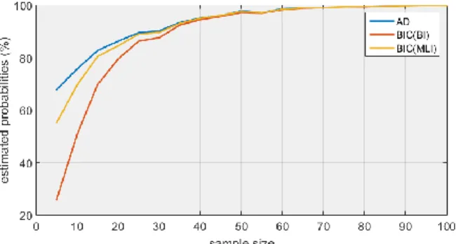
proportions are in fact estimated probabilities because of the finite number of Monte Carlo steps. The results are gathered in Fig .2. (f1) and Fig. 3 (f2 and f3).
Whatever the test, the proportions increase with n. If n is large enough, all these tests are similar. The results of the AD and the BIC (MLI) are relatively close as they are both using the MLI. Whatever the test, the proportions converge quicker to 100% with f1 than with f2 and f3. If there is at least one
negative realization within the sample (only possible with f1 )
Fig. 2. Estimated probabilities of choosing N if the true distribution is N (f1)
Fig. 3. Estimated probabilities of choosing LN (resp. W) if the true
distribution is LN (f2) (resp. W (f3))
For f1, AD has the highest proportion of success, closely
followed by the BIC(MLI). The success rate of the BIC(BI) for very small samples are very low.
For f2, AD has again the highest success rate but the
BIC(MLI) is very similar. The performance of the BIC(BI) is again poor for small samples
For f3, the BIC(BI) has high proportions of success, even
for very small n, whereas the AD and BIC(MLI) fail most of the time.
For the N and LN distribution it seems that the MLI performs better than the BI. For the W distribution it is best to use the BI. In order to complete the comparison, the performance of the quality of the inferences estimators should also be studied. Such analysis (not shown in this paper) could modulate this conclusion.
As mentioned in section II, the N and LN are biased corrected estimators whereas the estimator of the W distribution is still biased since its quite complex correction was not implemented. Therefore, the Bayesian inference for the W distribution in this context is an easy way to improve the performance of the uncorrected classical estimator.
V. EMC APPLICATION
In the previous simulation, the random generation was totally controlled. The true distribution (its type and parameters) were known. In practice, it is obviously not the case. Moreover it is very difficult to test a large number of equipment. Therefore we will never be able to obtain the true distribution with real equipment. That is why we suggest a
virtual example as an application to test the BI and MLI. The random generation of susceptibility thresholds comes from an electromagnetic simulation of electronic equipment. It is an intermediate case between the theoretical simulation performed in section IV and a real case with susceptibility measurements. In the following example, the true distribution function is unknown as it is usually the case. However, we can simulate much more copies of equipment than it would be possible to test in practice. The example has to be simple enough so the simulation time is relatively short. The large sample allows us to obtain an estimation of the true distribution. Therefore this estimation can be considered as a pseudo-reference for smaller samples retrieved from the large sample. The inferences are tested on these smaller samples. We consider this example as an application since it is made of an electronic equipment (even if it is simple and arbitrary) and most of all, the variability of the susceptibility threshold is generated by variation of physical parameters.
We designed simple electronic equipment presented in Fig. 4.
Fig. 4. Virtual equipment
The equipment is a printed circuit board with two microstrip lines L1 and L2. L1 is ended by matched resistive loads. L2 is ended at one end by a resistor and at the other one by a transistor. L2 is entirely covered by a protective shielding whereas L1 is only covered partially. A small aperture is made at the shield interface so that the microstrip line gets out the shielded box. The uncovered portion of L1 is illuminated by a electromagnetic continuous plane wave, at 500MHz, with normal incidence and polarized in the parallel direction to the uncovered portion of the line L1. Underneath the shielding, L1 and L2 are close to one another which cause a crosstalk coupling. The nominal dimensions of the design are: L1=205, L2=130mm, the ground plane has an area of 250 x 250mm and the Fr4 substrate thickness is 1.7mm.
The equipment variability is ensured by the randomness of multiple parameters (lines length, charges, parasitic capacitor of the transistor [18]…) around the design nominal value (variability arbitrary set to 10%). Therefore, each device is a random realization.
The field intensity is raised until provoking a failure. The failure criterion is associated to the output (Vds) of a transistor mounted as a reverser. When no constraint is applied, the input voltage (Vgs) is at 0V and therefore the output (Vds) is at 5V. The transistor is blocked. If Vds is lower than an arbitrary
threshold Vth the transistor is no longer considered blocked and this is considered as equipment failure.
We were able to simulate nc=2000 copies of that equipment. We call that sample the reference sample. nc was chosen to be much larger than samples of size n of interest (a few tens) but not too large to be compatible with reasonable simulation times (about 6 hours). With Vth=4V, the nc simulated thresholds are represented in Fig. 5. The choice of
Vth only translates (and preserve the shape) the thresholds distribution to higher levels if Vth decreases for example.
Fig. 5. Reference susceptibility distribution
A fitting with the three distributions is also plotted. The W and N distribution seem both fitting well (at least visually) the data. The LN fitting is further away from the empirical distribution. The CV is equal to 23.45%. We showed on Fig.1 that W and N distribution are in fact very similar for CV closed to 30%.
We proceed now to a Monte Carlo study. At each step we randomly selected n equipment from the nc sample. We then apply the BI and the MLI. We select the hypothesis corresponding to the minimum BIC. Once all Monte Carlo computations are performed, we compute the proportions of good decisions. As evidenced in Fig. 5, W and N distributions fit better the data than a LN distribution. That is why a good decision is choosing N or W, whereas choosing LN is considered as a bad decision. The results are gathered in Tab.2.
TABLE I. PROPORTIONS OF GOOD / BAD DECISIONS (%)(IN GREEN / RED
COLOURS) n 5 10 15 BIC (BI) Hi=N 0.9 5.2 9.3 Hi=L 13.4 12.9 11.4 Hi=W 85.7 81.9 79.3 BIC (MLI) Hi=N 31.4 38 40.9 Hi=L 52.1 37.7 28.2 Hi=W 16.5 24.3 30.9
The BI rejects more often the L distribution than the MLI for the three tested n. Moreover, even if it is not crucial here, the BI seams to select more often W than N whereas the MLI selects more often N than W.
In practice we have only one small sample. As mentioned in section II, both of them can lead to a probability density function of the estimated parameter. As a consequence, the estimated cdf of the susceptibility may be rather considered as a beam of plots. More than identifying the most probable
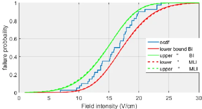
susceptibility distribution, it is relevant to express the bounds of the estimated cdf. Both inferrences (BI and MLI) give a multivariate density of the distribution parameter. Therefore the failure probability at a certain constraint level is also a density. At each constraint level, the quantiles of the failure probability can be computed. In Fig. 6 we plot the 95% interval of confidence for both inferences with one sample of 20 equipment copies. The bounds resulting from the BI are slightly narrower than those resulting from the MLI. As the sample size increases (40 in Fig. 7 and 100 in Fig. 8), the bounds are narrower and the BI and MLI lead to the same bounds.
Fig. 6. Empirical distribution (ecdf) and estimation of the upper and lower bound of the failure probability for both inferrences and a sample of 20 equipment
Fig. 7. Empirical distribution (ecdf) and estimation of the upper and lower bound of the failure probability for both inferrences and a sample of 40 equipment
Fig. 8. Empirical distribution (ecdf) and estimation of the upper and lower bound of the failure probability for both inferrences and a sample of 100 equipment
From the point of view of the susceptibility analysis, both inferences method lead to similar bounds of the susceptibility distribution.
VI. CONCLUSION
This paper is dedicated to the statistical inference of the susceptibility distribution of electronic equipment when the number of equipment available for test is small. The goal of the study was to estimate the distribution type from a limited set of susceptibility thresholds. We wanted to determine which approach, the Bayesian or the maximum likelihood, was best suited in that case. By Monte Carlo we applied the two inferences in order to select one distribution amongst three possibilities. Thanks to the selection criterion BIC we selected the most probable distribution. When the true distribution is either N or LN, the MLI is more effective than the BI, whereas when the true distribution is W it is the opposite. In the context of a particular case example, we showed that the BI is the best to rejects LN. This was expected according to the estimation of the distribution from a large sample. Finally, thanks to the posterior distribution of the estimated parameter from both inferences, the failure probability can be bounded. This information can be useful in the context of EMC failure risk analysis.
However, this paper did not study the quality of the two inferences estimators. A comparison of their mean and variance should be done in order to further compare the two inferences and quantify the conclusion. Moreover in the Bayesian inference we used non informative priors. If prior knowledge is available (previous experiences, expert opinion…) the Bayesian inference can take it into account and most likely improve the performance. This is not possible with the maximum likelihood inference.
ACKNOWLEDGMENT
The authors would like to acknowledge the support from the DGA.
REFERENCES
[1] C.F.M. Carobbi, "Bayesian Inference in Action in EMC—Fundamentals
and Applications", IEEE Trans. On EMC. Vol. 59, no 4, p. 1114-1124,
2017
[2] C. Yuhao, L. Kejie and X. Yanzhao, "Bayesian assessment method of
device-level electromagnetic pulse effect based on Markov Chain Monte Carlo", APEMC 2016 Electromagnetic Compatibility (APEMC), 2016
Asia-Pacific International Symposium on. pp. 659-661, 2016
[3] T.W Anderson and D.A. Darling, "A Test of Goodness-of-Fit", Journal of the American Statistical Association, Vol. 49, n°268, pp. 765–769, 1954.
[4] G. Casella, R. L. Berger, "Statistical Inference", 2nd edition chapter 7.
[5] J-J. Ruch, “Statistique: Estimation”, Preparation for the Agrégation Bordeaux 1. 2013 p.11.
[6] L. Perreault and B. Bobée, "Loi Weibull à deux paramètres Propriétés
mathématiques et statistiques Estimation des paramètres et des quantiles Xr de période de retour T", Scientific report n° 351 1992.
[7] H. Hirose, “Bias Correction for the Maximum Likelihood Estimates in
the Two-parameter Weibull Distribution”, IEEE Trans. On Dielectrics
and Electrical Insulation Vol. 6, n°1, p. 66-68, 1999.
[8] E. T. Jaynes, "Prior Probabilities", IEEE Trans. on Systems Science and Cybernetics Vol. 4, n°3, pp. 227-241, 1968.
[9] A. R. Syversveen, "Non informative Bayesian Priors. Interpretation
And Problems With Construction And Applications", Preprint Statistics , vol. 3, pp. 1-11 1998
[10] A. Zellner, “Maximal data information prior distributions”, (A. Aykac and C. Brumat, eds.), New developments in the applications of Bayesian methods pp. 211 232, 1977.
[11] H. Jeffrey, "An invariant form for the prior probability in estimation
problems", Proceedings of the Royal Society of London a: mathematical, physical and engineering sciences, The Royal Society, pp. 453-461 1946.
[12] J. Berger and J. Bernardo, "On the development of the reference prior
method", Bayesian Statistics, Vol. 4, n°4, pp 35-60, 1992.
[13] R. Yang and J. O. Berger, “A Catalog of Non informative Priors”,
Institute of Statistics and Decision Sciences, Duke University, pp. 97-42,
1998.
[14] A. Zellner, “Bayesian and non-Bayesian analysis of the log-normal
distribution and log-normal regression”, Journal of the American
Statistical Association, Vol. 66, n° 334 327– 330, 1971
[15] E. Fabrizi and C. Trivisano, “Bayesian Estimation of Log-Normal
Means with Finite Quadratic Expected Loss”, Bayesian Analysis Vol. 7, n°4, p. 975-996, 2012.
[16] N. M. Razali and Y. B. Wah, "Power comparison of shapiro-wilk
kolmogorov-smirnov lilliefors and anderson-darling tests", Journal Of Statistical Modeling and Analytics, Vol. 2, n°1, pp. 21-33, 2011.
[17] K. BurnHam and D.R. Anderson, "Multimodel Inference Understanding
AIMV and BIC in Model Selection", Sociological Methods&Research Vol. 33, n°2, 261-304, 2004.
[18] C. Pouant, "Caractérisation de la susceptibilité électromagnétique des
étages d’entrée de composants électroniques", PhD Thesis pp.103, pp. 163-168 2015.
View publication stats View publication stats