HAL Id: hal-01420790
https://hal.archives-ouvertes.fr/hal-01420790
Submitted on 21 Dec 2016
HAL is a multi-disciplinary open access
archive for the deposit and dissemination of
sci-entific research documents, whether they are
pub-lished or not. The documents may come from
teaching and research institutions in France or
abroad, or from public or private research centers.
L’archive ouverte pluridisciplinaire HAL, est
destinée au dépôt et à la diffusion de documents
scientifiques de niveau recherche, publiés ou non,
émanant des établissements d’enseignement et de
recherche français ou étrangers, des laboratoires
publics ou privés.
A comparison of cost construction methods onto a
C6678 platform for stereo matching
Judicaël Menant, Guillaume Gautier, Jean-François Nezan, Muriel Pressigout,
Luce Morin
To cite this version:
Judicaël Menant, Guillaume Gautier, Jean-François Nezan, Muriel Pressigout, Luce Morin. A
com-parison of cost construction methods onto a C6678 platform for stereo matching. 2016 Conference
on Design and Architectures for Signal and Image Processing (DASIP), Oct 2016, Rennes, France.
�10.1109/DASIP.2016.7853821�. �hal-01420790�
A comparison of cost construction methods onto a
C6678 platform for stereo matching.
Judica¨el Menant
IETR / INSA Rennes jmenant@insa-rennes.fr
Guillaume Gautier
IETR / INSA Rennes gugautie@insa-rennes.fr
Jean-Franc¸ois Nezan
IETR / INSA Rennes jnezan@insa-rennes.fr
Muriel Pressigout
IETR / INSA Rennes mpressig@insa-rennes.fr
Luce Morin
IETR / INSA Rennes lmorin@insa-rennes.fr
Abstract—Stereo matching techniques aim at reconstructing depth information from a pair of images. The use of stereo matching algorithms in embedded systems is very challenging due to the complexity of state-of-the-art algorithms.
Most stereo matching algorithms are made of three different parts; the cost construction, the cost aggregation and the dis-parity selection. This paper focuses on comparing the efficiency of different cost construction methods implemented on a Digital Signal Processor (DSP) C6678 platform.
Three cost construction algorithms based on census, Sum of Absolute Differences (SAD) and Mutual Information (MI) have been compared in terms of output quality and execution time. Each method has its own specificity discussed in this paper. The SAD is the simplest one and is used as reference in this paper. The census has a good output quality, and the MI is faster.
INTRODUCTION
Embedded vision is the merging of two technologies cor-responding to embedded systems and computer vision. An embedded system is any microprocessor-based system that is not a general-purpose computer [1]. The goal of our work is to implement computer vision algorithms in modern embedded systems to provide them with stereo perception.
There are two ways to obtain Red Green Blue and Depth (RGBD) information onto embedded systems: either active devices such as Kinect or stereo matching algorithms that compute depth information from two or more images. Active systems[2] emit an infra-red grid on the observed scene. The disparity map is then deduced from this sensed-back grid. Those devices are limited to indoor use with a 5 meter range and they are sensitive to infrared interferences. This paper focuses on binocular stereo vision algorithms to bypass these limitations.
Stereo matching aims to create 3D measurements from two 2D images, generating a disparity map which is inversely proportional to the depth of any object to the acquisition system. Disparity maps are used in a wide range of scenarios where depth must be computed (3D TV, free-view point video,...). There are two main classes of stereo matching algorithms, the dense one and the sparse one. Sparse stereo matching algorithms consider only a set of interest points whereas dense stereo matching algorithms match all pixels. In this paper we consider only dense stereo matching algorithms as they are used in most 3D applications.
Most existing implementations of dense stereo matching algorithms are carried out on desktop Graphical Processor
Unit (GPU), leading to poor energy efficiency. On top of that the GPU used for the implementations are different so that it is very difficult to really compare the complexity of the algorithms. Embedded systems take up little space and consume little power, so they are ideal for widespread integration into everyday objects. Energy-efficient embedded platforms are now available. The C6678 platform is a recent 8-core Digital Signal Processor (DSP) platform at the state of the art in the field. The C6678 is clocked at 1 GHz with a standard 10W power consumption. However, the architecture of embedded systems is significantly different to the architec-ture of desktop systems. The challenge is therefore to find and adapt algorithms and implementations that can fully exploit the powerful computational capabilities of such an architecture. To be efficiently implemented on embedded systems, algorithms must be ported to fixed point implementation. Fixed point implementations lead to quantification noise and quality loss, thus a trade-off between precision and quality must be found. As it will be further exposed, stereo matching algorithms are divided into three main algorithms. The cost construction, the cost aggregation, and the disparity selection. The goal of this paper is to compare the implementation efficiency of different cost construction algorithms in terms of quality and computing complexity using the same DSP platform (C6678). Three different stereo matching cost construction algorithms are considered. These three algorithms are at the state of the art in the field of stereo matching algorithms [3].
First, a short overview of stereo matching principle is introduced followed by the presentation of the C6678 in section II. Then, each chosen algorithm is explained in section III. After this non-exhaustive presentation of stereo matching algorithm, the results are exposed, execution times and quality output for each algorithm. To finish the perspectives and future work are exposed.
I. STEREO MATCHING PRINCIPLE
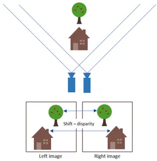
In order to retrieve depth information from two stereoscopic images, stereo matching algorithms find the correspondences between those two images. When the stereoscopic system is rectified, the disparity is the shifting of the two corresponding pixels in the left and the right images (see figure 1). The bigger the disparity is, the closest the object is from the two cameras. Dense stereo matching algorithms are mainly divided into two classes, local and global methods [3]. The disparity
Fig. 1: Disparity in stereoscopic images
computed with a local method depends only on colorimetric values of pixels within a finite window. Semi-global stereo matching algorithms maximize smoothness of the disparity map all over the image. The memory constraint of embedded systems does not allow the use of global algorithms so it will not be studied in this paper.
All dense stereo matching algorithms can be divided into three main parts :
• The cost construction measures the similarity of two pixels considering the colorimetric values of those pixel and a finite neighborhood.
• The cost aggregation refines costs taking into account the neighbourhood and adds consistency between the disparity values.
• The disparity selection deduces the disparity level for a
given pixel from the costs produced by the previous steps. Three state-of-the-art stereo matching cost construction al-gorithms are studied in this paper:
• The Mutual Information (MI) (part III-A) is a semi-global method that computes a Look Up Table (LUT) based on joined probability of the two images to get the cost.
• The Sum of Absolute Differences (SAD) (part III-B ) is a simple and very commonly used local method.
• The census (part III-C) is a more robust method that gives good results for stereo matching.
II. THEC66X MULTI-COREDSPPLATFORM
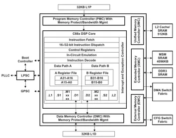
The c6678 platform is composed of 8 c66x DSP cores and it is designed for image processing. Figure 2 gives an overview of this platform. The main features and constraints (memory architecture and DSP core) of this widespread multicore platform have to be recalled because they explain why the algorithms have to be modified to be efficiently executed on any embedded systems.
Fig. 2: C6678 DSP block diagram
A. Memory architecture
Memory is a critical point parameter in embedded systems. Large memories being slower than smaller ones, modern systems integrate several memory layers in order to increase the memory capacity without increasing the access time to data too much. The memory hierarchy of the c6678 platform is exposed below :
• 512 MBytes of external DDR3 memory. This memory is slow, and the bus bandwidth is limited to 10 GBytes/s. This memory is shared between all 8 cores. It is con-nected to the 64-bit DDR3 EMIF bus.
• 4 MBytes of internal shared memory (MSMSRAM). It
is a SRAM memory and it is very fast : its memory bandwidth is 128 GBytes/s .
• 512 KBytes of L2 cache per core. It can be configured as cache or as memory, and it is very fast. In this paper this memory is configured as cache.
• 32 KBytes of Data L1 cache and 32 KBytes of Program L1. They are zero wait state caches (one transfer per machine cycle).
B. DSP Core
In this section, the main specific architecture points of c66x cores are introduced.
1) VLIW: The C66x DSP has 8 fully independent Arith-metic and Logic Unit (ALU) (see figure 3). This implies that the core is able to execute up to 8 instructions simultaneously in one cycle with a mechanism named Very Long Instruction Word (VLIW). The core is composed of two independent data paths with 4 ALU.
In most digital signal processing applications, a loop kernel is a succession of interdependent sequential operations. In order to use efficiently the VLIW architecture, these loops
Fig. 3: C66x DSP core
must be pipelined, that is to say, several iterations of the core loop are done simultaneously, and thus parallelized. Loop pipelining is done by the compiler. A speed-up factor of 6 can be easily achieved with a little human work. However a loop can’t be pipelined when it contains jumps or conditional statements. These rules must be kept in mind when writing efficient code and when designing algorithms.
2) SIMD: Single Instructions Multiple Data (SIMD) are instructions that are executed on multiple data. A SIMD instruction considers one or two registers (32 or 64 bits respectively) as a set of smaller words. For instance a 32-bit register can be seen as a group of 4 8-bit words, and is called a 4-way 8-bit SIMD instruction. This kind of instruction is very useful in image processing because most of the manipulated data is 8-bit (pixels). The use of SIMD instructions usually involve a loss in terms of accuracy compared with floating point instructions.
3) FPU: The Floating Point Unit (FPU) is a logic unit which is able to execute operations on floating point numbers. The c66x has a basic FPU ; Nevertheless, this FPU has low support of SIMD (two ways maximum), whereas SIMD on fixed point numbers is up to 8 ways. Moreover a floating point number is always 4 bytes wide, thus causes a higher memory usage.
C. Implementation strategies for stereo matching
The development on this platform is done using C language. When specific instructions need to be used such as SIMD, C intrinsics are used.
All stereo matching algorithms have the same structure, and different strategies can be applied to parallelized it. All stereo matching algorithms can be sliced vertical without increasing the memory footprint. Nevertheless some algorithms can lead in synchronization penalties between slices.
Most of local stereo matching algorithms have their cost computed independently for each disparity level. Those algo-rithms can be parallelized along their disparity levels. This
parallelization is very effective. However it comes with an increase in terms of memory footprint.
A specific Digital Signal Processor (DSP) instruction can be used to increase the implementation efficiency of algorithms for instance the bit count instruction for census, or the min instruction for saturation.
Finally, a pixel-level parallelization is possible to compute several pixels simultaneously thanks to SIMD instructions. Implementation and performances of this solution depend on the concerned algorithm.
In the next sections we will describe the three considered stereo matching algorithms which have been implemented and compared.
III. ALGORITHMS
As introduced previously, the dense stereo matching algo-rithms rely on three steps :
• The cost construction.
• The cost aggregation.
• The disparity selection.
This section introduces the three selected cost construction algorithms, the cost aggregation and the disparity selection studied in this paper.
A cost construction algorithm provide a cost for each possible matching pixel pairs. The lower the cost is, the most likely the math of the corresponding pixel pair is.
A cost construction algorithms has two stereoscopic images at input : Ib(p) and Im(p). Ib(p) is the base image (the left
image in this paper) image, and Im(p) is the image to be
matched (the right image in this paper).
For all pixels p = (x, y) in the base image, all the possible matches are pixels p0= (x − d, y) in the image to be matched, where d varies among all possible disparities values, 0 to D (the maximum number of disparity) in this paper.
The output of a cost construction algorithm is a cost matrix Cost(p, d) of size W ×H ×D where W and H are respectively the horizontal and vertical size of an image.
A. Mutual Information (MI)
The first studied cost construction algorithm is the Semi Global Matching (SGM) one. It has been developed by Heiko Hirshm¨uller[4], and uses a matching cost based on a Mutual Information (MI) to compensate the radiometric differences of input images. The aim of the algorithm is to create a Look Up Table (LUT), mi cost matrix.
As explained previously, the MI based cost construction takes two stereoscopic images as input, but also a disparity map. The disparity map is the final results of a stereo matching algorithm, thus, a stereo matching algorithm that uses a MI based cost becomes recursive.
The principle of MI based cost construction, is to build from mutual information of pixel a 256 by 256 LUT. The the intensities of two pixels are used as input of this LUT to retrieve the corresponding matching cost.
MI based cost construction’s input images I1 and I2 are
is the function that moves each pixel intensity according to the disparity map. PI1,I2(i, k), where (i, k) are the coordinates of
the matrix, is an histogram defined as :
PI1,I2(i, k) = 1 n× X p T [(i, k) = (I1(p), I2(p))] (1)
PI1,I2(i, k) represents the probability distribution of the
different couples of intensities (I1, I2) and T [ ] is an operator
which is ’1’ if (i, k) = I1(p), I2(p), 0 otherwise. The algorithm
counts the number of pixels of possible combinations of intensities, then, this sum is normalized by the number of existent couples. n is the number of corresponding pixels. First, a Gaussian filter is applied to the probability PI1,I2(i, k),
then a logarithm. The aim of this step is to smooth the result and to decrease the gap between values.
hI1,I2(i, k) = −
1
n× log (PI1,I2(i, k) ⊗ g(i, k)) ⊗ g(i, k) (2)
hI(i) is the entropy of each image, and is retrieved from
PI1(i) and PI2(k) as shown in equation (3). PI1(i) and PI2(k)
are the sum of the correspondent rows and columns of the joint probability distribution PI1(i) =
P
kPI1,I2(i, k).
hI(i) = −
1
n× log (PI(i) ⊗ g(i)) ⊗ g(i) (3) The matrix mii1,i2 (equation (4)) is the LUT that is used to
retrieve cost, and contains the probability of having a certain couple of intensities (I1, I2).
miI1,I2(i, k) = hI1(i) + hI2(k) − hI1,I2(i, k) (4)
This matrix allows to compute the cost. For each pixel p = (x, y) and disparity d, the cost matrix is defined as :
CM I(p, d) = −mi(Ib(x, y), Im(x − d, y)) (5)
The different costs computed with this formula are stored in the cost matrix.
Implementation details: The cost construction based on MI is mainly based on a LUT that is almost optimal. Nevertheless an efficient implementation of the construction of the LUT is proposed.
In order to build the histogram, 16 bits words are used, this allows the use of 4 ways Single Instructions Multiple Data (SIMD) in the further processing (Gaussian filters). The construction of histogram is easily parallelized by cutting input images in slices.
In order to use only integer words, the normalization of histogram is skipped. Indeed, a multiplying factor does not change the results because the only operations done with those costs are comparisons.
The logarithm scale is computed using a 8-bits LUT.
B. Sum of Absolute Differences (SAD)
This second cost computation algorithm is the simplest one. The Sum of Absolute Differences (SAD) [3] compares radiometric values of pixels at position (x, y) and at position (x − d, y). This algorithm performs a fully local calculation without considering neighbourhood, so it is very sensitive to noise and image variations.
sim(x, y, d) = |Ib(x, y) − Im(x − d, y)| (6a)
CSAD(p, d) =
(
thres, if sim(x, y, d) ≥ thres sim(x, y, d), otherwise
(6b) The thres is a constant linked to the noise level of image, 20 is generally a good value [3].
Implementation details: The SAD cost construction is very simple, 8-bits SIMD is used, and it is easily parallelized (Very Long Instruction Word (VLIW) and multi core).
C. Census Cost
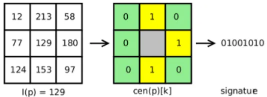
The third and last cost computation method is the census cost [5], [6], [7]. It considers its closed neighbourhood, the local texture, during its computation and can be computed efficiently on a VLIW DSP core. This algorithm is applied on a window N × N where N is odd. As shown in figure 4, this signature is obtained by comparing each pixel to its N2− 1 neighbours. The census is referred as cenm , cenr
in equation (7) for respectively Ib and Imgrey level images.
Fig. 4: 8 bits census signature example
In order to retrieve the cost from cenb and cenr, the
differences between the signature of two pixels are counted as shown in equation (7). CCEN(p, d) = 1 m m−1 X k=0 (
0 if cenr(x, y)[k] = cenm(x − d, y)[k]
1 if cenr(x, y)[k] 6= cenm(x − d, y)[k]
(7) where m = N × N − 1
The size N of the census window is parametrizable, in this paper three different values are tested : 3, 5 and 7.
Implementation details: The census cost construction has two separate steps. The first one computes the census signature for all the pixels of the two input images. The second one computes the cost from those signatures.
The construction of cenm and cenr is complex but must
be done only once for a stereoscopic pair. In order to speed up this construction the 8 ways SIMD instruction ”dcmpgtu4”
is used. This instruction is able to compare simultaneously 8 bytes and store the results in a 8 bits word were each bit is the result of the comparison. This is exactly what census does.
The comparison of two signatures is very simple, it is a eXclusive OR (XOR) followed by a bitcount (”bitc4”) instruction.
D. Bilateral Filtering Aggregation (BFA)
The second step in the dense Stereo Matching process is the cost aggregation one. The studied method in this paper is chosen to have a low computing cost, but it provides noisy matching cost maps. To reduce this noise, the cost Bilateral Filtering Aggregation (BFA) step performs smoothing on areas with similar colour in the original image. It has been originally proposed by Mei[5], [8]. The cost aggregation step is performed independently on each disparity level. This is a key point regarding implementation and its memory footprint. This algorithms fits very well on a c6678 platform [7]
The cost aggregation algorithm’s structure is similar to a bi-lateral filter. The cost aggregation step is performed iteratively with varying parameters. It is defined by equation (8).
Ei+1(p) =
W (p, p+)Ei(p+) + Ei(p) + W (p, p−)Ei(p−)
W (p, p+) + 1 + W (p, p−)
(8) Ei is the current cost map to be refined, E0 is the output
of cost construction.
Pixels p+ and p− have a position relative to pixel p : • p+= p + ∆i
• p−= p − ∆i
Equation (8) is computed alternatively for horizontal and vertical aggregations :
• When i is odd, it is a vertical aggregation and the offset ∆i is vertical.
• When i is even, it is an horizontal aggregation and the offset ∆i is horizontal.
At each iteration the parameter ∆igrows, thus further pixels
p+ and p− are used for smoothing p. ∆i evolves according
to equation (9), the influence range is limited by the modulo (here ∆i∈ [0, 32]).
∆i= f loor(i/2)2mod 33 (9)
Weights W in equation (8) are defined by equation (10) : W (p1, p2) = eCd.∆i−sim(p1,p2).L −1 2 (10) where sim(p1, p2) = s X col∈(r,g,b) (Ircol(p1) − Ircol(p2))2 (11)
In equation (10), Cd is a weight applied to distance[5]
and L2 is the weight applied to similarity [5]. Ir{r, g, b} and
Il{r, g, b} are the RGB (Red, Green, Blue) signals of right
and left images.
E. Disparity selection
The disparity selection step minimizes the matching cost. The Winner Takes it All (WTA) strategy [3] is used. The WTA strategy is a simple arithmetic comparison expressed by equation (12). Because the Bilateral Filtering Aggregation (BFA) cost aggregation step provides a good quality cost, a simple disparity selection like WTA can be used.
Disp(p) = argmin
d∈[0,N disp]
Ed,N it(p) (12)
The output of the disparity selection is a dense disparity map providing an integer disparity value for each pixel in the right image.
The BFA work on one disparity level at a time, thus, it is not necessary to store the whole disparity matrix in memory.
IV. RESULTS
The three selected cost construction algorithms and their implementation particularities are explained in section III. The Sum of Absolute Differences (SAD) is the most commonly used cost construction algorithm in literature[3] and is used as reference. The Census is a more robust cost algorithm, that fits very well on the C66x architecture. The Mutual Information (MI) based cost uses a Look Up Table (LUT) that decreases the number of operation during the cost matrix construction.
This are not a test.
Each cost construction is experimented using the Bilateral Filtering Aggregation (BFA) and Winner Takes it All (WTA) disparity selection. Thus, all output quality changes are in-duced by the cost construction steps.
Experimentations are run on a computer with a CPU Intel I7-4770 @3.40GHz and on a C6678 Digital Signal Processor (DSP).
To quantify the output quality, the Middlebury [3] evaluation tool and dataset are used. This paper exposes the percentage of bad pixels and separates occulted area from not occulted area. The execution times are given for the sawtooth image (380*432) with 19 disparity levels. The output quality is an average of six images : cones, map, venus, tsukuba, teddy and sawtooth. times on Sawtooth PC time(ms) DSP time(ms) SAD 24,52 5,0 MI 23,34 6,7 Census 3x3 58,69 8,1 Census 5x5 134,80 17,5 Census 7x7 235,74 35,3
Fig. 5: Observed times on PC(CPU @3.40GHz) and DSP In figure 5, the execution time provided for the MI based cost is for one iteration. As explained in section III-A, stereo matching algorithms that use a MI based cost construction are iteratives. Experiences show that 5 iterations are required to have a good disparity map. Nevertheless it is possible to down
sample the input images, and up sample the disparity map at each iteration, this gives an execution overhead inferior to 1.5 [9]. This is not a problem in a video application because the input can be the disparity map from the previous frame.
In figure 5, we found, as expected, times that are coherent with the complexity of the algorithms. All the algorithms are sensitive to the size of the images but the census execution time also depends on the size of its window and,like the SAD, to the number of disparity levels. In all the algorithms compared in this article only the MI is not really sensitive to the disparity parameter, because during the construction of the cost matrix, the algorithm just fetch the value in the precomputed LUT.
Estimated algorithm complexities:
• SAD: O(H.W.D)
• MI: O(H.W.D)
• Census N × N : O(H.W.D.N2)
Average scores on Middlebury set bad pixels(%) non-occulted(%)
SAD 13,23 9,11
MI 10,92 10,77
Census 3x3 19,14 15,23 Census 5x5 8,43 4,48 Census 7x7 7,27 3,39
Fig. 6: Observed scores with Middlebury tool In order to get better quality results, the size of the census window is increased at 5x5 and at 7x7 window. The result obtained are over 2,5% of bad pixels less compared to MI.
The three algorithms have their ins and their outs, but this observation can be done: the MI is the best when you have a constraint of time. When you need good quality result, the 7x7 census or even the 5x5 are better. The other algorithms are less time efficient compared to the MI and the census.
All the result images with the different cost can be found on the last page in figure 7.
CONCLUSION ANDFUTURE WORK
A. Conclusion
This paper compares the efficiency of three different costs construction onto a C6678 Digital Signal Processor (DSP) platform. The three cost construction algorithms studied are based on census, Mutual Information (MI) and Sum of Abso-lute Differences (SAD).
The three algorithms have there pros and cons even if we can just retain two of them: MI et census. The speed of those algorithms is evaluated on a PC platform and a c6678 DSP platform. Their quality is also compared thanks to the Middlebury evaluation tools [3].
As exposed in the part IV, the MI is faster than the others, but several iterations are required except on a video application. The best quality is achieved with a 5x5 or 7x7 census cost. However, the census is quite slow on PC, but fits
well on the DSP architecture. It gives really good scores (over 3% less than the MI based cost).
The actual experiment set up has a major drawback, it is very bad on occulted area. There are disparity selection algorithms that takes into account occulted area such as belief propagation [10] or SGM [6]. Those algorithms work generally on large cost matrix. Implementing them onto a DSP with limited high speed memory is challenging.
REFERENCES
[1] E. V. Alliance, “What is embedded vision.” http://www.embedded-vision.com/what-is-embedded-vision.
[2] K. Khoshelham and S. O. Elberink, “Accuracy and resolution of kinect depth data for indoor mapping applications,” Sensors, vol. 12, no. 2, pp. 1437–1454, 2012.
[3] R. S. Daniel Scharstein, “A taxonomy and evaluation of dense two-frame stereo correspondence algorithms,” International Journal of Computer Vision, no. 47, pp. 7–42, 2002.
[4] H. Hirschmuller, “Accurate and efficient stereo processing by semi-global matching and mutual informaition,” IEEE Computer Society Conference on Computer Vision and Pattern Recognition (CVPR), jun. 2005.
[5] X. Mei, X. Sun, and M. Zhou, “On building an accurate stereo matching system on graphics hardware,” in Computer Vision Workshops (ICCV Workshops), 2011 IEEE International Conference on, nov. 2011, pp. 467 –474.
[6] I. Ernst and H. Hirschm¨uller, “Mutual information based semi-global stereo matching on the gpu,” in Proceedings of the 4th International Symposium on Advances in Visual Computing, ser. ISVC 08. Berlin, Heidelberg: Springer-Verlag, 2008, pp. 228–239.
[7] J. Menant, M. Pressigout, L. Morin, and J.-F. Nezan, “Optimized fixed point implementation of a local stereo matching algorithm onto c66x dsp,” in Design and Architectures for Signal and Image Processing (DASIP), 2014 Conference on, Oct 2014, pp. 1–6.
[8] J. Zhang, J.-F. Nezan, M. Pelcat, and J.-G. Cousin, “Real-time gpu-based local stereo matching method,” in conference on Design and Architecture for Signal and Image Processing, Cagliary, October 2013.
[9] H. Hirschmuller and D. Scharstein, “Evaluation of stereo matching costs on images with radiometric differences,” Pattern Analysis and Machine Intelligence, IEEE Transactions on, vol. 31, no. 9, pp. 1582–1599, Sept 2009.
[10] J.-F. Nezan, A. Mercat, P. Delmas, and G. Gimel’farb, “Optimized belief propagation algorithm onto embedded multi and many-core systems for stereo matching.” in Parallel, Distributed, and Network-Based Processing (PDP), 2016, Conference on, 2016.
Cones Teddy Sawtooth Tsukuba
Cones with SAD Teddy with SAD Sawtooth with SAD Tsukuba with SAD
Cones with MI Teddy with MI Sawtooth with MI Tsukuba with MI
Cones with Census3x3 Teddy with Census3x3 Sawtooth with Census3x3 Tsukuba with Census3x3
Cones with Census5x5 Teddy with Census5x5 Sawtooth with Census5x5 Tsukuba with Census5x5
Cones with Census7x7 Teddy with Census7x7 Sawtooth with Census7x7 Tsukuba with Census7x7