HAL Id: hal-02427017
https://hal.archives-ouvertes.fr/hal-02427017
Submitted on 3 Jan 2020
HAL is a multi-disciplinary open access
archive for the deposit and dissemination of
sci-entific research documents, whether they are
pub-lished or not. The documents may come from
L’archive ouverte pluridisciplinaire HAL, est
destinée au dépôt et à la diffusion de documents
scientifiques de niveau recherche, publiés ou non,
émanant des établissements d’enseignement et de
A Condition-Based Dynamic Segmentation of Large
Systems using a Changepoints algorithm: A Corroding
Pipeline case
Rafael Amaya-Gómez, Emilio Bastidas-Arteaga, Franck Schoefs, Felipe
Munoz, Mauricio Sanchez-Silva
To cite this version:
Rafael Amaya-Gómez, Emilio Bastidas-Arteaga, Franck Schoefs, Felipe Munoz, Mauricio
Sanchez-Silva. A Condition-Based Dynamic Segmentation of Large Systems using a Changepoints algorithm:
A Corroding Pipeline case. Structural Safety, Elsevier, 2020, �10.1016/j.strusafe.2019.101912�.
�hal-02427017�
A Condition-Based Dynamic Segmentation of Large Systems using a
Changepoints algorithm: A Corroding Pipeline case
Rafael Amaya-G´omeza,b,⇤, Emilio Bastidas-Arteagab, Franck Schoefsb, Felipe Mu˜nozd, Mauricio S´anchez-Silvac
aChemical Engineering Department, Universidad de los Andes, Cra 1E No. 19A-40, Bogot´a, Colombia
bUniversit´e de Nantes, GeM, Institute for Research in Civil and Mechanical Engineering, CNRS UMR 6183, Nantes, France cDepartment of Civil & Environmental Engineering, Universidad de los Andes, Cra 1E No. 19A-40, Bogot´a, Colombia
dEmpresa Colombiana de Petr´oleos (ECOPETROL) S.A., Cra 7 No. 32-42, Bogot´a, Colombia
Abstract
Large structures are systems composed by a significant number of components with parallel or series distributions. How these components fail and interact, aggravate the complexity of the main structure reliability calculation. Some methods commonly proposed to reduce this complexity by dividing the system into segments of similar properties using dynamic or static approaches. Dynamic segmentations may depend on how aggressive is the structure’s sur-rounding conditions (e.g., the soil properties). Static segmentations could be given by fixed distances. However, in a few cases, these divisions follow a condition-based approach. This paper proposes an alternative dynamic segmenta-tion to identify preliminary critical segments based on a Changepoint approach and data obtained from inspecsegmenta-tions. Changepoints algorithms have been used to determine changes in spatial measurements for a further reliability eval-uation with appropriate limit state functions. This work focuses on onshore pipelines subjected to corrosion defects based on information obtained from In-Line Inspections (ILI). Onshore pipelines cross through a variety of soils, water corridors, and densely populated areas promoting spatial-dependent degradation processes like corrosion. ILI inspections are commonly used to identify the condition of the pipeline in terms of the remaining wall and location of metal loss at the inner and outer walls by using magnetic or ultrasonic instruments. Based on a burst failure limit state, the segments obtained with the changepoints approach are compared with a soil and static segmentations. The results indicate that the proposed approach could identify the main critical points of the pipeline using segments with statistical significance.
Keywords: Reliability, Dynamic segmentation, Changepoints, Corroding pipeline
1. Introduction
1.1. Large structures context
Large structures are systems composed by a set of parallel or serial components (or subsystems) that define the serviceability of the entire structure. Some examples include onshore/offshore pipelines, where commonly segments from 10 to 14 meters are joint together in series using welding processes. Also, sheet piling harbors use parallel steel sheets as a retaining wall and pavement sections in steel or reinforced concrete structures like bridges. Reliability of large structures is quite complicated; even the definition of failure could use cumbersome expressions. In some cases even asymptotic perspectives have been considered, where the number of components is assumed to tend infinity, aiming to find some limit reliability forms [1]. For instance, consider a series system with n components that can fail independently from each other with a reliability R1, . . . ,Rn. The reliability of the system is obtained as the product
of the reliability of each defect, Rp=Qni Ri, which means that the failure probability (i.e., the complementary of the
reliability) would tend to 1 for a significant number of components, although they have an almost negligible failure
⇤Corresponding author,
Email address: [email protected] (Rafael Amaya-G´omez)
Please cite this paper as:
Amaya-Gómez R, Bastidas-Arteaga E, Schoefs F, Muñoz F, Sánchez-Silva M. (2020). A Condition-based Dynamic Segmentation of Large Systems using a Changepoints algorithm: A Corroding Pipeline case. Structural Safety 82:101912 1-15. https://doi.org/10.1016/j.strusafe.2019.101912
probability. This pattern should attract much attention for treats like corrosion, considering that it is one of the top priorities for steel structures like underground onshore/offshore pipelines and those exposed to marine environments, e.g., sheet piling harbors [2–5].
Corrosion reduces the thickness of the steel, making it prone to a plastic failure or even a rupture or collapse, depending on the applied loads such as the operating pressure, surrounding stresses, or climate conditions. Corrosion is a time and space-dependent phenomenon that depends on several factors including the properties of the soil, the metabolic activity of microorganisms or fungi, and the presence of imperfections on the steel or stray currents. For instance, soils with a higher concentration of chlorides, sulfates, acidic pH, and the presence of bacteria or fungi have a significant effect on external corrosion on steel pipelines [6]. Also, water pollution and temperature have been acknowledged to influence accelerated low water corrosion (ALWC), and immersion corrosion on sheet piling harbors [2]. The challenge relies on the fact that steel structures usually cover extensive distances, especially for onshore/offshore pipelines, where pipeline routes can reach distances up to 4700 km (e.g., Eastern Siberia-Pacific Ocean oil pipeline). These structures may pass through a variety of soils, water corridors, and densely populated areas. The varied soil conditions surrounding the structure and the way the structure is installed (e.g., underground, aboveground) and maintained, also affect the space-dependent degradation process during its life-cycle, which has raised several efforts regarding their modeling, maintenance, and repair [3, 7, 8].
1.2. Corroding pipeline integrity
Inspection plays a significant role in future interventions by updating the structure condition and allowing decision-makers to evaluate the current maintenance, repair, and inspection planning. In this direction, different inspection and assessment strategies have been proposed to prioritize critical sections [9–11], in some cases, even considering sampling or partial inspections [12]. Specifically for onshore pipelines, Oil & Gas companies implement In-Line (ILI) inspections using a set of magnetic (Magnetic Flux Leakage, MFL) or ultrasonic (UT) sensors to provide information about the size and location of the defects detected along the pipeline. This information serves to assess the current condition of pipelines based on different empirical, numerical, or probabilistic approaches. Empirical approaches usually cover standards or best practices of Oil & Gas companies; see for instance [13, 14]. Numerical approaches usually deal with Finite Elements simulations, and probabilistic approaches evaluate plastic collapse, yielding, or leak failure criteria based on safety margins or limit state functions (see [15–18]). In either case, these analyses aim to support decisions for integrity management and pipeline risk analysis.
Risk analyses for corroded pipelines consider how likely is a Loss of Containment (LOC) based on the metal thinning and the consequences it may follow. The likelihood could be estimated using historical records as the number of LOCs given the timespan and distance traveled by the fluid (i.e., failures/km·year); another common alternative follows a spatial-dependent probabilistic perspective with a segmentation that assumes a constant behavior per segment. The consequences would depend on the accidental scenario given by, for example, the pipeline height, soil conditions, and release mode [19].
1.3. Segmentation of corroding pipelines
Segmentation is the process of defining pipe sectors with similar characteristics (external or internal) that can be used as units for integrity evaluation. Segmentation can be static – i.e., initially predefined–, or dynamic - i.e., adaptable to mechanical or external conditions. Static segmentations use fixed distances defined arbitrarily (e.g., 1 km), or by specific mechanical elements of particular interest such as valves. In static segmentation, there is considerable variability in the results of risk assessment and may increase intervention costs due to unnecessary evaluations. In the dynamic segmentation, the length is not relevant as long as the feature on which the segmentation is evaluated remains constant throughout the entire segment [20]. A dynamic segmentation seems to be more reasonable for corroded steel, where localized defects are common along to the structure.
A segmentation provides valuable information for decision-makers regarding future pipeline interventions in quan-titative risk analysis in terms of how segments are prioritized, and maintenance planning is supported. Different cri-teria to segment the pipeline, including design, operating, and external soil conditions, have been proposed. Some of the reported approaches that segment the pipeline for analysis of reliability or consequence are summarized in Table 1. Note that in the absence of information, failure frequency rates can be used as a preliminary assessment, but these segments would only consider the pipeline age and not the real pipeline condition.
Table 1: Pipeline segmentation criteria
Source Segmentation criterion Classification
Sahraoui et al. [21] Soil type Dynamic
Hicks & Ward [22] Op. Pressure Dynamic
Diameter Dynamic
Wall thickness Dynamic
Age of pipeline Dynamic
Coating condition Dynamic
Soil conditions Dynamic
Population density Dynamic Mart´ınez et al. [23] Pig stations Static Bonvicini et al.
[24] Soil type Dynamic
Ground water table Dynamic
Leak position Static
De Leon & Flores
Mac´ıas [25] Every 10 km Static
Shan et al. [26] Population density Dynamic
Soil corrosivity Dynamic
Coating condition Dynamic
Liang et al. [27] Density of population Dynamic High Consequence Areas (HCA) Dynamic Changes in the pipeline laying Dynamic
Age of pipeline Dynamic
Soil conditions Dynamic
The available dynamic segmentations commonly divide the pipeline based on the type of soil, population density, or pipeline design features [28]. Nevertheless, few works divide the pipeline considering the current condition of the pipeline; in this regard, Amaya-G´omez and co-workers proposed a continuous segmentation following reliability projections [29]. Wang and co-workers [30] developed a framework to cluster defects depending on their corrosion rates, which are later used to estimate a space-dependent corrosion rate probability density. This approach considers defect measurements obtained from In-Line (ILI) inspections but also require high sensitive sensors to evaluate the soil conditions along the pipeline abscissa. This work also focuses on segments with critical sections based on the likelihood of a LOC, after an ILI inspection takes place. The consequences were not contemplated in this work bearing in mind that critical segments should be identified and later prioritized to avoid any LOC, unnecessary shutdown, or costly repair. This process would contemplate the possible effects given a LOC (i.e., thermal radiation, overpressure, or toxic dispersion), but they are out of the scope of this work due to significant uncertainty [31, 32].
1.4. Objective and paper structure
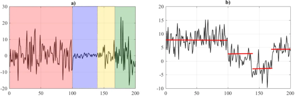
A sound partition should consider segments that depend on both the size of the defects and the number of defects per segment. For this purpose, a Changepoint Analysis is proposed in this work following the PELT (Pruned Exact Linear Time) method reported by Killick et al. [33] based on the size of the defects detected with an inspection. This algorithm aims to identify the jumps where statistical parameters like the mean or variance change based on a set of measurements as it is illustrated in Figure 1.
The approach proposed can be used as a screening tool to make a preliminary identification of critical segments in large structures, considering that this information should be validated using field measurements. The main contri-butions of this paper can be summarized as follows:
• The proposed approach is an alternative to segment large structures in the main direction given inspection results. The approach seeks to support further reliability evaluation using appropriate limit state functions. Besides, it can be used jointly with a consequence-based segmentation based on high consequence areas, main-tenance sensitive locations, or the position of fixed elements such as valves to identify sections with inadequate risk levels.
• This work proposes a dynamic segmentation for corroding pipelines using a condition-based approach based on the depth, length, and width of the defects for the first time. Previous approaches, consider pipeline segments
Figure 1: Scheme of changepoints based on the a) variance and b) mean of the data.
based on consequence rather than reliability perspectives such as the population density or the river-crossings. These additional changepoints can be incorporated into the approach if required.
• The paper compares the proposed approach with other segmentation techniques using pipeline soil distribution and a fixed segmentation. This comparison considers the lack of detailed information on a low scale of soils and how broad categories may not provide enough information regarding the corrosion aggressiveness. Also, this comparison highlights that fixed approaches do not capture possible variations along the pipeline, and even misleading results can be obtained because of the number of defects per segment.
The document is structured as follows: Section 2 presents the proposed segmentation approach based on ILI mea-surements and the changepoints algorithm. Section 3 describes the case study and its spatial dependencies. Section 4 shows the results and discussion using the case study and compares the results with two additional segmentation. Finally, conclusions and future perspectives are given in Section 5.
2. Dynamic segmentation based on the Changepoint algorithm 2.1. Proposed approach overview
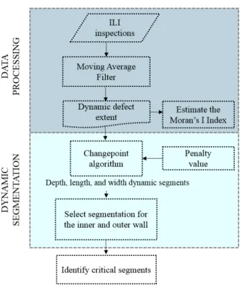
The methodology for the proposed dynamic segmentation is divided into two main stages, as is depicted in Figure 2, which have been used for structural inspections to characterize system spatial variability [34–36]. First, data pro-cessing is developed based on the defect depth, length, and width from each pipe wall reported at the ILI. Second, the dynamic segments are determined using the Changepoint algorithm subject to a penalty value to identify preliminary critical segments. This methodology will be described in more detail below.
2.2. Data processing
2.2.1. Data gathering - In-Line inspections
In pipelines, the primary testing procedure used to evaluate the evolution of corrosion with time is Line In-spections. ILI measurements provide valuable information about the condition to support operating and maintenance decisions. According to the Pipeline Operators Forum (POF) [37], the result of an ILI contains a pipe tally, list of anomalies, and a list of clusters. The pipe tally presents a list of all pipeline and anomaly features, which include: (i) Location and orientation parameters, (ii) structural parameters, and (iii) information regarding anomalies. The list of anomalies describes the anomalies found above the inspection tool reporting threshold. This list includes information regarding the geometric size of the defects (i.e., width, length, and depth), their location, and orientation using a clock-position analogy. Finally, a defect-cluster classification is provided in the list of defects following the ASME B31G criterion, which considers a relative distance less than 6t longitudinally or circumferentially to cluster two defects, where t stands for the intact pipeline wall thickness [37].
Figure 2: Proposed methodology using the changepoints algorithm
2.2.2. Preliminary segmentation - Moving Average Filter
As it was depicted in Figure 1, the changepoints algorithm identifies the location where the mean or variance changes for a set of measurement in a principal direction. Corrosion defects lie in a ”2D-plane” following a cylindrical fold with different metal loss measurements along the abscissa main direction, which means that a highly noisy ”signal” is foreseen. This noisy set of measurements would represent a significant number of changepoints that would overfit a further segmentation. Because this segmentation aims to identify relevant jumps regarding defects dimensions, a Moving Average Filter is applied to the data obtained from the ILI runs. This filter is one of the most used for signal processors; it produces an output signal from the average of M-sample points from an input signal. Formally, consider as the input signal a set of L measurements x1, . . . ,xLassociated with the depth, length, or width
that are sorted in the abscissa direction (i.e., a1 · · · aL), and M be a positive odd integer such that M ⌧ L. The
filtered signal would be given as follows: yi= 1 M (M 1)/2X j= (M 1)/2 xi+ j, i = (M 1) 2 +1, . . . , L (M 1) 2 (1)
As M grows, a smoother output signal would be expected where sharp transitions are well defined, but a poor ”frequency response” of the measurement may also occur if this parameter is very high. For practical purposes, it is assumed that M = d 0.01 L e, i.e., as the ceiling or higher nearest integer of the 1% of the number of measurements. Because this number may be quite small, let M = max (31, d 0.01 L e) to assure a filtering process that is statistically more significant.
2.2.3. Moran’s Index Evaluation
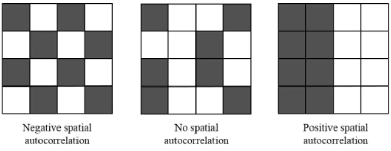
The preliminary segmentation is evaluated using the Moran’s Index, which is a global measure of spatial autocor-relation, based on the corrosion defects measurements (depth, length, and width) and their locations on the pipeline. The possible correlations are classified as positive, negative, or no spatial autocorrelation considering a dispersed,
random, or clustered distribution as is illustrated in Figure 3. For the sake of simplicity, these measurements would be represented by x. Consider a set of observations x1, . . . ,xMuse as part of the input signal and denote its average
as ¯x. The Moran’s index is then given by the ratio between a measure of the covariance of the observations and the corresponding variance [38]: I = M S0 PM i=1PMj=1wi j(xi ¯x)(xj ¯x) PM i=1(xi ¯x)2 , (2)
where S0=PMi=1PMj=1wi j, and W = [wi j] is a matrix of weights such that PMj=1wi j =1, for i = 1, . . . , M. Particularly,
wi jcorresponds to the weight of xjused to calculate the weighted average of xi[38]; thus, it follows that wii=0, 8i.
Figure 3: Spatial autocorrelation scheme
Assuming that the moments of Moran’s Index can be estimated by permuting M! times the actual observations and that there is no spatial autocorrelation (Null Hypothesis), these moments are given by [38]:
E(I) = (M 1)1 , (3) 2(I) = M[(M2 3M + 3)S1 MS2+3S20] k[M(M 1)S1 2MS2+6S20] (M 1)(M 2)(M 3)S2 0 , (4) where, S1= 12 M X i=1 M X j=1 (wi j+wji)2, (5) S2= M X i=1 0 BBBBB B@ M X j=1 wi j+ M X j=1 wji 1 CCCCC CA 2 , and (6) k = 1/M P M i=1(xi ¯x)4 h 1/M PM i=1(xi ¯x)2 i2. (7)
Based on these moments, the null hypothesis (no spatial autocorrelation) can be assessed using the expected value of the observations. For this work, the functions included in the Analyses of Phylogenetics and Evolution (APE) library in R-project were used to calculate the Moran’s Index with the following considerations:
1. xi=(ai,pi), where aiand piare the defect position at the pipeline abscissa and the perimeter, respectively; and
2. wi j= 1
2.3. Dynamic segmentation
2.3.1. Changepoint algorithm overview Consider a sequence of data yn
1 =(y1, . . . ,yn) and suppose that m changepoints were determined with positions
⌧m1 =(⌧1, . . . , ⌧m), where ⌧i2 {1, . . . , n} correspond to y’s ordered index (i.e., ⌧i< ⌧jif and only if i < j) [33]. Then,
the data is divided into m + 1 segments that are not necessarily equally separated. These changepoints are commonly determined by minimizing the following expression [33]:
m+1
X
i=1
[C(y⌧i
(⌧i 1+1))] + f (m), (8)
where C is a cost function that depends on the segment evaluated and f (m) is a penalty factor to avoid overfitting, which for the linear case is used as f (m) = m with a constant penalty value. This cost function can follow different approaches, but commonly the log-likelihood is used. In this regard, the changes in the mean can be evaluated through the cost of segments given a common variance 2as in Eq. 9 [39]. According to Haynes et al. [39], the first term of
this cost function can be omitted to obtain a square error cost. C(yt(s+1)) = (t s) log 2+ 12 t X j=s+1 0 BBBBB @yj 1 t s t X i=s+1 yi 1 CCCCC A 2 . (9)
There are different approaches to find the optimal segments such as the Segmented Neighborhood (SN), the Optimal Partitioning (OP), Binary Segmentations (BS), and the Pruned Exact Linear Time method (PELT). From these approaches, PELT was selected because it is an efficient and versatile method in comparison to other approaches [33].
2.3.2. Selection of the Penalty value The sequence of data yn
1is associated with the mean depth, length, and width of the defects. The mean was chosen
considering the significant variability along the pipeline abscissa and possible exaggerated number of segments if a maximum criterion was used, especially for the defect length and width. The changepoint algorithm depends on a penalty value that is initially unknown (Eq. 8), but it has a direct relation to the number of changepoints: a higher penalty value would represent a fewer number of changepoints for the PELT partitioning. To deal with this parameter, the CROPS (Changepoints for a Range of Penalties) algorithm of Haynes et al. [39] was implemented with the PELT optimal splitting. This algorithm finds the optimal number of changepoints for intermediate penalties intervals given minimum ( min) and maximum ( max) values as it was proved by Haynes et al. [39] (see Theorem 3.1).
The outcome of the CROPS algorithm is a series of optimal segmentations from intermediate penalty values given [ min, max]. The best segmentation is chosen following the recommendations used by Lavielle [40] and Haynes et al.
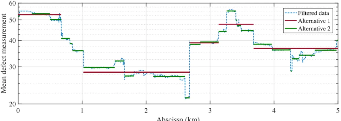
[41], which consider a sensitivity analysis using the segmentation cost and the number of changepoints. Recall that the cost decreases as the number of changepoints rises, so a function C = h(m) would have an ”elbow” or point of maximum curvature that avoids significant false-positive jumps on the final segmentation, i.e., some segments with a small cost reduction. These jumps are illustrated in Figure 4 for the second alternative of segmentation; for instance, note that around the third kilometer, there is a changepoint for a marginal difference in the mean defect measurement. The point of maximum curvature is estimated using a non-parametric fitting of h(m) with cubic splines and finite differences. Cubic splines are used to approximate h(m) continuously following a log-log scale to avoid any scaling problem, whereas finite differences are used to estimate its first two derivatives and calculate the curvature as follows (where a prime represents a derivate d
dm):
= |C00|
1 + C02 3/2. (10)
For this work, the Least-squares spline modeling functions slmengine and slmeval developed by John D’Errico [42] are used because several knots can be imposed, which in turn, follow an optimal location. This number of knots is set as the half number of points obtained from CROPS, but again because a relatively short segment may be initially selected, this number is suggested to be as low as 100.
0 1 2 3 4 5 Abscissa (km) 20 30 40 50 60
Mean defect measurement
Filtered data Alternative 1 Alternative 2
Figure 4: Scheme of two segmentation alternative with low and high number of changepoints.
2.3.3. Pipeline segmentation
Once the penalty values are chosen, the next step focuses on determining a dynamic segmentation based on the results from the defect depth, length, and width. Basically, the changepoints are merged in one segmentation and those segments with less than 30 defects are joint together to the nearest segment. Formally, let do
1 := {d1, . . . ,do},
l1p:= {l1, . . . ,lp}, and wq1:= {w1, . . . ,wq} be the segmentations from the defect depth, length, and width, and define the
ordered union of these segmentations as U := sort({do 1,l
p 1,w
q
1}), which without loss of generality, can be denoted as
u1,u2, . . . ,uo+p+q. Estimate the number defects within each of these elements including u0=0 and uo+p+q+1=Lp; i.e.,
the defects from the ILI in the segments Uj=[uj,uj+1] for j = 0, . . . , (o+ p+q). If there exist a j where the number of
points kUjk 30, then ujor uj+1should be deleted depending on which of them is closer to uj 1or uj+2, respectively.
The reader should bear in mind that a near intact pipeline may produce a segmentation with few changepoints, so the analysis can be limited to the affected area.
2.4. Reliability-based critical segments
For each of the segments obtained previously, a failure probability following a plastic collapse are assessed, aiming to identify segments likely to fail. A plastic collapse considers a pressure-based limit state (i.e., g = Pb Pop) between
the pipeline burst pressure (Pb), in which the pipe wall will bulge outward and reach a point of instability, and the
pipeline operating pressure (Pop). If g 0 the system is in a failure state, whereas if g > 0 is in a safe mode.
The failure probability of an entire segment, PS egf , would be bounded as follows. Let P1
f, . . . ,Phf denote the failure
probability of h defects in a given segment, then max {P1 f, . . . ,Phf} PS egf 1 h Y i=i (1 Pi f). (11)
The lowest bound considers a failure of completely correlated defects, whereas the upper bound assumes that the failure of each defect is independent of each other. Although these bounds could be broad estimations and there are other narrower approximations [43], this approach is considered for illustrative purposes.
3. Spatial dependencies of the case study 3.1. Main parameters
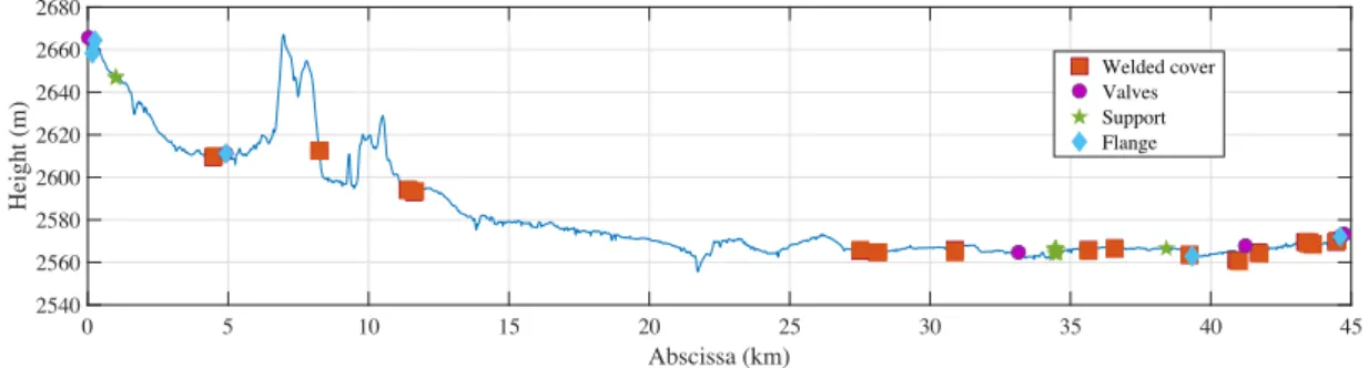
The case study concerns an API 5LX52 pipeline 45km long, its height lies between 2560 to 2660m above the sea level, and it has six main valves. The pipeline has welded covers, supports, and flanges along the route, as shown in Figure 5. The pipeline is mainly localized in a plain terrain with inclinations lower than 7 , it crosses two mountain sections, and two urban zones. The climate is mainly cold dry, but there are also cold-humid zones. The mean length for the pipe joints is 10.7m, and the welded cover is 0.7m. The location of the welded covers, the supports, and valves
near kilometer 33 are associated with a river crossing, whereas the last 10km are close to urban zones. The pipeline has a nominal wall thickness of 6.35mm and an external diameter of 273.1mm. The analysis presented here was based on data obtained from two consecutive ILI measurements two years apart. According to the ILI report, this diameter is maintained along the entire abscissa, while the wall thickness exhibits greater variability due to the location of welded covers, valves, dents, and manufacture flaws. The defects measuring tool was a Magnetic Flux Leakage (MFL). Based on information reported in Amaya-G´omez et al. [15] about the inspection vendor, it can be assumed a circumferential uncertainty of 5 during the inspection. The measurement uncertainties of the defect depth, length, and width are given by dILI =dreal± ✏d, lILI =lreal± ✏l, and wILI =wreal± ✏w, where dILI,lILI,wILIstand for the depth, length, and width
reported by the ILI tool, and ✏d, ✏l, ✏ware the measurement errors. The measurement errors can be assumed to follow
normal distributions centered at 0 with standard deviations obtained from the inspection vendors [44]. It is reasonable to assume that ✏d = 0.1 t with t the nominal wall thickness, ✏l = ✏w = 11.70mm, considering a length and width
accuracy of 15mm with a confidence of 80% of the data. For confidential agreements, further details of the case study cannot be provided. 0 5 10 15 20 25 30 35 40 45 Abscissa (km) 2540 2560 2580 2600 2620 2640 2660 2680 Height (m) Welded cover Valves Support Flange
Figure 5: Pipeline main parameters based on the abscissa and height.
Regarding the pipeline operation, Figure 6a shows that both ILI inspections report small fluctuations in the mean operating velocity (around 2.2 m/s). Figure 6b depicts slightly higher differences in temperature from 27 to 34 C. Following the results of authors like Qi et al. (2014) [45] and Prawoto et al. (2009) [46], higher corrosion rates would be expected near 5km and 22km, where the highest temperatures are reported.
0 5 10 15 20 25 30 35 40 45 Abscissa (km) 26 27 28 29 30 31 32 33 34 Operating temperature (°C) b) ILI 1 ILI 2 0 5 10 15 20 25 30 35 40 45 Abscissa (km) 1 1.2 1.4 1.6 1.8 2 2.2 2.4
Mean operating velocity (m/s)
a)
ILI 1 ILI 2
Figure 6: a) operating velocity and b) temperature along the abscissa.
Table 2 shows a broad classification of the soil along the pipeline following the taxonomy of the USDA (United States Department of Agriculture). The pipeline has a bituminous coating of coal tar and an impressed current cathodic protection (ICCP) system. Coal tar is composed principally of aromatic hydrocarbons that constitute the foremost the liquid condensate of the distillation process from coal to coke [47]. Coal-tar-based coatings have exceptional moisture resistance; however, some disadvantages of these coats are poor light stability and possible cracks at the upper surface coming from an oxidation process due to a higher level of unsaturation [47]. Thicker layers can protect the pipeline, but a process of delamination is expected in a higher proportion than a polyethylene coat [48].
Table 2: Pipeline segmentation based on the USDA soil classification
Segment* Category Classification ID
0.00-6.66km Complex Pachic Melanudands (50%), Andic Dystrudepts (20%), Aeric Endoaquepts (15%), AquicHapludands (15%) Soil 1 6.66-8.2km Association Humic Lithic Eutrudepts (35%), Typic Placudands (25%), Dystric Eutrudepts (25%) Soil 2 8.2-9.66km Complex Pachic Melanudands (50%), Andic Dystrudepts (20%), Aeric Endoaquepts (15%), AquicHapludands (15%) Soil 1 9.66-11.61km Association Humic Dystrudepts (60%), Typic Hapludalfs (40%) Soil 3 11.61-13.48km Complex Pachic Haplustands (35%), Humic Haplustands (35%), Fluventic Dystrustepts (30%) Soil 4 13.48-14.86km Association Aeric Epiaquents (60%), Fluvaquentic Endoaquepts (40%) Soil 5 14.86-15.89km Complex Humic Dystrustepts (40%), Typic Haplustalfs (35%), Fluvaquentic Endoaquepts (25%) Soil 6 15.89-17.62km Association Aeric Epiaquents (60%), Fluvaquentic Endoaquepts (40%) Soil 5 17.62-18.65km Complex Humic Dystrustepts (40%), Typic Haplustalfs (35%), Fluvaquentic Endoaquepts (25%) Soil 6 18.65-18.84km Association Typic Endoaquepts (40%), Aeric Endoaquepts (30%), Thaptic Hapludands (20%) Soil 7 18.84-21.40km Complex Humic Dystrustepts (40%), Typic Haplustalfs (35%), Fluvaquentic Endoaquepts (25%) Soil 6 21.40-22.63km Association Typic Endoaquepts (40%), Aeric Endoaquepts (30%), Thaptic Hapludands (20%) Soil 7 26.07-27.35km Complex Pachic Haplustands (35%), Humic Haplustands (35%), Fluventic Dystrustepts (30%) Soil 4
27.35-28.22km Urban zone -
-28.22-30.52km Association Aeric Epiaquents (60%), Fluvaquentic Endoaquepts (40%) Soil 5 30.52-33.10km Complex Pachic Haplustands (35%), Humic Haplustands (35%), Fluventic Dystrustepts (30%) Soil 4 33.10-35.45km Association Typic Endoaquepts (40%), Aeric Endoaquepts (30%), Thaptic Hapludands (20%) Soil 7
35.45-45.00km Urban zone -
-*Both ILI did not include information of the segment from 22.63 to 26.07km
3.2. Main descriptors of corrosion defects
The majority of defects are concentrated on the inner wall, which is somehow expected due to the coal-tar coating; a summary statistics of these data sets is depicted in Table 3. Because further information about defects shape is not available in ILI, the maximum rather than the average depth for each defect will be considered from now on.
Table 3: Summary of corrosion defects along the abscissa
Parameter ILI-1 Inner wall ILI-2 Inner wallMean (Coefficient of Variation)ILI-1 Outer wall ILI-2 Outer wall Average depth (%t) 5.49 (0.26) 5.29 (0.27) 7.28 (0.49) 6.77 (0.46) Maximum depth (%t) 11.54 (0.21) 11.14 (0.19) 15.84 (0.46) 14.62 (0.43) Length (mm) 26.07 (0.49) 26.07 (0.43) 28.07 (0.48) 27.37 (0.44) Width (mm) 22.5 (0.40) 25.92 (0.53) 28.81 (0.67) 32.60 (0.75)
Number of defects 23708 43399 2862 4264
The corrosion defects were classified following the categories reported by the Pipeline Operator Forum [37], and their primary metal descriptors were compared. These categories include general corrosion, pitting, axial (ferential) grooving, pinhole, and axial (circum(ferential) slotting. Large and wide defects may be related to circum-ferential/axial grooving or even general corrosion. Table 4 depicts the distributions of these categories where it can be noticed that general and pitting corrosion cover around 90% in both inspections and pipe walls, but there is still a relevant number of axial and circumferential grooving at the inner wall. The absence of pinholes and slotting de-fects (both axial and circumferential) may suggest that ultrasonic tools were implemented for both inspections [49]. However, MFL tools were used instead, and circumferential slotting defects are actually included in these ILI reports, but their corresponding dimensions do not fit into the POF boundaries for this defect type, so this classification was ignored.
Following the categories mentioned above, the defect depth was compared again for each inspection and pipe wall obtaining the results detailed in Table 5. This table indicates that defects classified as general corrosion and circumferential grooving have a considerable proportion of profound defects, whereas axial grooving defects tend to be less profound. This table also suggests that the outer wall from both inspections have a significant variability, which could be attributed to the number of defects, soil aggressiveness, and the extreme conditions at the river-crossing. Besides, the mean and coefficient of variation for the defect depths in the outer wall are similar than those reported for the outer wall and that the mean depth decrease between the two consecutive inspections. These results
Table 4: Defects classification according to their size
Category ILI-1 Inner wall ILI-2 Inner wallNumber of defects (%Total defects)ILI-1 Outer wall ILI-2 Outer wall
General 2007 (8%) 5766 (13%) 515 (18%) 891 (21%)
Pitting 19551 (82%) 34460 (79%) 2116 (74%) 2997 (70% )
Axial Grooving 1920 (8%) 2007 (5%) 164 (6%) 125 (3%)
Circumferential Grooving 230 (1%) 1166 (3%) 67 (2%) 271 (6%)
can be explained based on a more homogeneous degradation process due to the transporting fluid and the appearance of new corrosion defects.
Table 5: Defect depth for each sizing category
Category Mean depth of defects %t (Coefficient of variation)
ILI-1 Inner wall ILI-2 Inner wall ILI-1 Outer wall ILI-2 Outer wall
General 12 (0.23) 11 (0.20) 17 (0.44) 15 (0.44)
Pitting 12 (0.22) 11 (0.19) 16 (0.45) 15 (0.42)
Axial Grooving 11 (0.18) 11 (0.14) 14 (0.25) 14 (0.31)
Circumferential Grooving 11 (0.27) 11 (0.21) 20 (0.73) 15 (0.54)
4. Results and discussion 4.1. Data processing
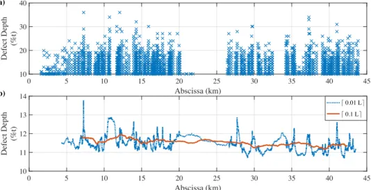
The Moving Average Filter was applied to each set of depth, length, and width measurements at both inspections and pipe walls. This filter reduces the ”noisy” input signal as it is illustrated in Figure 7 for the depth of the defects at the inner wall of the first ILI run. The choice of M (i.e., max (31, d 0.01 L e)) assures a sharp profile that is useful for the Changepoint approach; a higher parameter may produce an overly smooth data that hide possible mean jumps as it can be seen for the case of d 0.1 L e.
0 5 10 15 20 25 30 35 40 45 Abscissa (km) 10 20 30 40 Defect Depth (%t) a) 0 5 10 15 20 25 30 35 40 45 Abscissa (km) 10 11 12 13 14 Defect Depth (%t) b) ⌈ 0.01 L⌉ ⌈ 0.1 L⌉
Figure 7: a) Corrosion depth for the ILI run-1’s inner wall and b) Moving Average Filter output
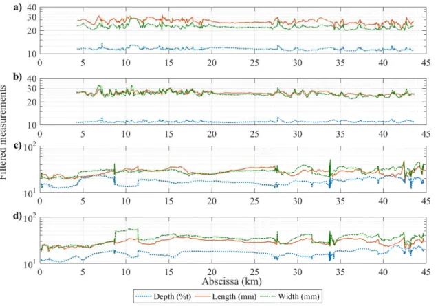
The filtered data depicted in Figure 8 show remarkable patterns for the mean depth, length, and width along the pipeline abscissa. Note, for instance, that near the eighth and tenth kilometers in the first ILI at the inner wall, there are pronounced peaks for the three corrosion measurements, whereas around the 36th kilometer these measurements decreased. These patterns are maintained for the second inspection at the inner wall, but defect depth reports more
stable results close to 10%t due to the generation of new defects and the repair of the most profound defects with welded covers. The outer wall results show more dispersed patterns for the depth, length, and width of the defects as a result of a significantly lower number of defects in comparison to the inner wall, particular degradation processes at the coal-tar coating, and the cross of a river.
Figure 8: Filtered measurements of the defect depth, length and width for a) ILI run-1’s inner wall, b) ILI run-2’s inner wall, c) ILI run-1’s outer wall, and d) ILI run-2’s outer wall.
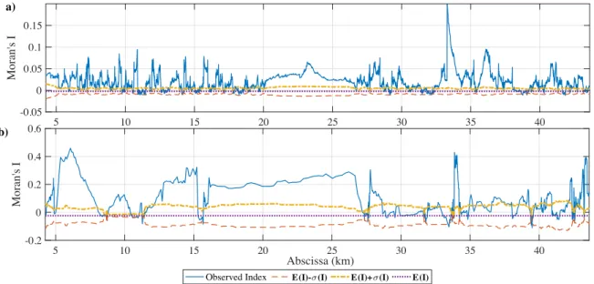
The Moran’s Index was calculated for the filtered segments considering a Null Hypothesis of no-spatial autocorre-lation or also named Completely Spatial Randomness. For this purpose, the observed Moran’s Index, and the expected indexes under the null hypothesis were determined and compared within each segment. Figure 9 depicts only the re-sults for the depth measurements at the inner and outer wall for the second inspection considering that similar rere-sults were obtained for the length and width of the defects. This figure includes a constant E(I) because the number of points for each segment was M, and two bounds given by E(I) ± (I). The results suggest that the segments tend to have a positive correlation (i.e., more clustered), especially for the outer wall, but some segments have weak spatial correlation as they lie within or near to this range. This result would support the use of the filter because they may capture clustered data instead of entirely different measurements.
4.2. Dynamic segmentation and evaluation
The R-project function cpt.mean was used to determine the optimal changepoints (number and location) given to a range of penalty values from min = 1 to an arbitrarily large number max = 10, 000 under CROPS approach [50]. This function also provides the decreasing cost of the segmentation based on the number of changepoints as is depicted in Figure 10 for the defects depth, length, and width for the inner wall at the first inspection. These costs were approximated to continuous functions using cubic splines based on the slmengine function, and their points of maximum curvature were determined for each case using finite differences. The results from each type of measurements, inspection, and pipe wall are shown in Table 6. Note that because the depth of the defects presents less
5 10 15 20 25 30 35 40 -0.05 0 0.05 0.1 0.15 Moran's I a) 5 10 15 20 25 30 35 40 Abscissa (km) -0.2 0 0.2 0.4 0.6 Moran's I b)
Observed Index E(I)-σ(I) E(I)+σ(I) E(I)
Figure 9: Observed and expected Moran’s Index for the a) Inner and b) Outer wall of the defect depth.
sharp jumps along the pipeline abscissa, the numbers of changepoints were lower than those for the length and width of the defects. 0 50 100 150 Changepoints 0 1000 2000 3000 4000 5000 Segmentation Cost a) 0 50 100 150 200 250 300 350 400 Changepoints 0 1 2 3 4 5 6 Segmentation Cost ×104 b) 0 50 100 150 200 250 300 350 400 Changepoints 0 1 2 3 4 5 Segmentation Cost ×104 c)
Figure 10: Changepoints vs. Segmentation cost for the defects a) depth, b) length, and c) width for the inner wall at the first inspection.
Table 6: Number of changepoints using a maximum curvature approach Measurements Inspection Pipe wall Changepoints
Depth ILI Run-1 Inner 34
Outer 29
ILI Run-2 Inner 27
Outer 24
Length ILI Run-1 Inner 47
Outer 50
ILI Run-2 Inner 57
Outer 32
Width ILI Run-1 Inner 42
Outer 34
ILI Run-2 Inner 58
For each dataset, the segments obtained from the defects depth, length, and width changepoints were merged seeking for segments with at least 30 defects. Based on these segmentations, the mean depth, length, and width of the defects for both inspections and pipe walls were determined and depicted in Figure 11 with their corresponding soil classes. Regarding the inner wall, Figure 11a shows that the mean depth oscillates mostly between 11 and 13%t for the first inspection and the second ILI measurement from 10.5 to 12%t. This reduction can be explained by the detection of new corrosion defects near the reporting threshold of 10%t and the repair of the more profound defects like those located at the 7th, 10-11th, and 17th kilometers. These segments were mostly associated with Soil 2, Soil 3, and Soil 7. Additionally, the defects crossing close the urban area reported relevant increments in both segments. Figure 11c depicts the mean length for the inner wall, where it can be noticed that the mean length overall lies between 22 and 32mm for both inspections. This figure indicates that the larger defects are in the kilometers 12, 14, and 35, which corresponds with the Soil 4, Soil 5, and Soil 7, but additionally, there are some larger segments reported close to the Soil 2 and the urban area. Finally, Figure 11e depicts the mean width obtained using the proposed segmentation. This figure displays a width between 20 and 30mm for the first inspection, whereas from 23 to 40mm for the second ILI. In contrast to the previous results, the width of the defects tends to increase between the two inspections. The wider defects are located near to the 11th (Soil 3) for both inspections and 7th kilometers (Soil 2) for the last inspection.
Regarding the results for the outer wall, Figure 11b depicts a higher variability on the depth of the defects than in the inner wall, obtaining mean measurements between 12 and 22%t. This segmentation has significant changepoints close to the 33rd kilometer, which are associated with the degradation of the river-crossing. The results indicate that the deeper defects are located from 5 to 9 km (Soil 1 and Soil 2) and from 34 to 43 km (Soil 7 and UZ) for the first inspection; after the repairs, an important depth increment occurred from 11 to 14 km (Soil 3 and Soil 4). Figure 11d illustrates that the length of the defects oscillate near 30mm, lying among 20 and 45mm. Besides, this figure indicates that the first kilometers (Soil 1) had the shorter lengths and the kilometer 42 report the longer defects. Finally, Figure 11f presents the results of the mean width for both inspections, displaying a clear increment between the two inspections (as in the inner wall). In addition, this figure shows some interesting results like the higher reported width in the Soil 3 (10-11km), Soil 7 (near the river-crossing), and the segment from 29 to 32 km (Soil 4 and Soil 5). Also, as in the mean length, it was reported the lowest results in the first five kilometers.
Although detailed comparisons with the soil properties are not possible due to a lack of information, it can be inferred that results may not depend markedly on the type of the soil considering the ranges from each case. Nonethe-less, the results from Figure 11 suggest that defects in Soil 2, Soil 3, Soil 5, and Soil 7 could be more aggressive than the other classes for the outer wall. The results from these soil categories also illustrate relevant variability within each soil category.
Overall, the challenge is choosing a satisfactory segmentation for the inner and outer wall to identify preliminary critical segments of the pipeline where more in-depth analyses should be proposed. Consider, for instance, a static segmentation every kilometer and also calculate the mean depth, length, and width as before (Figure 12). This figure indicates that the length of the defects at the inner wall lied almost exclusively near 25mm for both inspections, but in the previous result we have identified some relevant changes even greater than 30mm, which were completely undetected. This pattern was also found for the depth and width at the 35th and 10th kilometers, respectively. Besides some hidden changes, note that critical segments may be complicated to prioritize given to the length of the segment evaluated; these segments may even have a limited number of defects reported.
4.3. Comparison of critical segments - A reliability approach
A burst failure probability was evaluated following the formulation detailed in Section 2.4 for the proposed dy-namic segmentation (Section 4.2), a fixed segmentation every kilometer, and segmentation using the soil categories (see Table 2) considering the Netto et al. model [51]. This selection was made considering that the case study has a moderate toughness and that previous prediction errors were quite low using FEM and experimental tests, which indi-cates that the model tends not to be conservative [16]. For this calculation, the failure probability was estimated using 10,000 Monte Carlo simulations for each reported defect, and the failure probability of each segment was bounded using Eq. 11. For this purpose, the defect depth (d), and length (l) from these inspections were considered upon the records of each segment, whereas the operating pressure (P), pipeline diameter (D), yield strength ( y), and the
wall thickness (t) were evaluated using random variables. The yield strength and the wall thickness use multiplicative random factors following lognormal distributions, i.e., y= ILIy · X yand t = tILI· Xt; all these random variables are
Figure 11: Mean depth (a) inner and b) outer wall), mean length (c) inner and d) outer wall), and mean width (e) inner and f) outer wall) based on the dynamic segmentation
Table 7: Case study random variables Parameter D [mm] Pop[MPa] X y[-] Xt[-]
Mean 273.1 10.34 1 1
COV 0.001 0.08 0.09 0.07
Distribution Normal Gumbel Lognormal Lognormal
The results are depicted in Figure 13. This figure illustrates how different segmentations based on the same information may affect further intervention decisions. The proposed segmentation captures the main jumps described by shorter fix segments. It leads to the computation of higher failures probabilities, which initially may suggest that this segmentation overestimates the reliability of the pipeline. However, recall that the main role of the segmentation is to identify segments that maintain a reliability level. Note that the failure probability for the defects located within the 10th and 15th kilometers are quite similar, so it can be assured that this pipeline segment follows similar reliability.
Figure 12: Mean depth (a) inner and b) outer wall), mean length (c) inner and d) outer wall), and mean width (e) inner and f) outer wall) based on a static segmentation every kilometer
Besides, each segment has at least 30 defects per segment, so more adequate failure predictions would be obtained than those using the other segmentations.
The approach proposed in this paper aims to be an alternative for segmenting onshore pipelines based on the valuable information obtained from ILI. This approach can be used with a corrosion degradation process to analyze how these segments evolve with time and how the maintenance planning may change as well. Once preliminary critical segments are identified, such as 10-15km based on a Low Safety Level according to DNV [52], more specific analyses can be considered including more detailed field measurements.
4.4. Additional remarks for leak and rupture limit states
This work evaluates the pipeline reliability only under a burst failure criterion, bearing in mind that no degradation process has been included so far; nevertheless, other release modes may occur like a small or large leak or even a full-bore rupture. If a probabilistic [15, 44] or stochastic [9, 53] degradation process is implemented, these limit state
functions can be assessed together. Let g1, g2, and g3denote limit state functions for a leak, burst, and rupture at an
individual corrosion defect, respectively:
g1=0.8t dmax,
g2=Pb P,
g3=Prp P,
where Pb denotes the burst pressure, Prp is the rupture pressure, and dmax is the maximum depth of the corrosion
defects. There are different approaches to estimate the burst pressure given to the metal toughness (see Appendix A), whereas the rupture pressure can be taken from CSA Z662 as follows:
Prp = 2t f
MfD,
where fstands for the flow stress (0.9 u) and Mf is the Folias factor of the CSA Z662 criterion. According to Zhou
et al. [54], these limit state functions can be used as follows to predict the failure modes: a small leak occurs when g1 0 and g2 > 0; a burst when g1 >0 and g2 0; a large leak when g1 >0, g2 0, and g3 >0; and a rupture
when g1 >0, g2 0, and g3 0 [54]. This classification varies slightly from the reported in CSA Z662, where small
leaks occur when the corrosion degradation process consumes the wall thickness completely. The failure probabilities for these limit states can be determined using Monte Carlo simulations or approximate methods like FORM/SORM for each obtained section. These results can be used with consequence-based segmentations (e.g., High Consequence Areas) and specific locations of interest like valve locations to identify locations where the risk may not be adequate.
5. Conclusions and future perspectives
This paper presented a dynamic segmentation strategy for large longitudinal structures (e.g., pipelines) that are frequently inspected. The approach uses inspection results under a Moving Average Filter, for reducing ”noisy” measurements per segment. Afterwards, the PELT (Pruned Exact Linear Time) method and the CROPS (Changepoints for a Range of Penalties) were used to identify mean jumps along the structure main direction. The case study considers a corroded pipeline that has been inspected internally with intelligent pigs (ILI). The measurements of the defect depth, length, and width were used to characterize the segmentation. The dynamic segmentation allowed identifying critical segments based on the burst failure criterion reported by Netto et al. [51]. Some of these sections were initially hidden in other segmentations based on the soil and a fixed partition every kilometer. Condition-based segmentations can provide valuable information about which sections of the pipeline are prone to fail, which can in turn, support further inspections and maintenance-based decisions.
The segmentation is defined from a reliability perspective, which could be later exploited for additional risk as-sessment evaluations, e.g., once failure consequences are contemplated and their spatial distribution is provided. For onshore pipelines, risk assessments may divide the pipeline considering sensitive locations in terms of high conse-quence areas. These divisions could include, for instance, the population density, how accessible is the location, or the possible environmental losses [55]; however, databases and incident frequency failures are commonly used to eval-uate a LOC. Few works address the spatial variability of the pipeline using condition-based analyses. Our approach focused on a reliability perspective aiming to prevent a LOC by identifying preliminary sections prone to fail, which in turn, would require further attention in their maintenance/inspection planning.
Future perspectives would seek to apply this approach with multiple limit states like small/large leak or pipe burst, once a corrosion degradation process is considered. This approach can be used jointly with consequence analysis to support maintenance and inspections, seeking optimal sections to intervene. Moreover, this approach can be applied to other large systems under a spatial-dependent degradation, considering a primary evaluation direction, and its inspection results. Some examples could be cracks in pavements or the condition of the sheet piling harbors, which are used as protection walls. Overall, large systems pose relevant challenges in reliability assessments, considering the number of components and the way we handle classic reliability perspectives. The reliability of system series like pipelines may be significantly small depending on the number of defects since it is obtained from their product. The complement of the reliability or failure probability would approach 1 (i.e., almost certain event), although the failure probability of all the defects lies on acceptable reliability criteria. In this direction, a segmentation or partition of a large structure allows a reduction of the complexity, given by a smaller number of components, which in turn, could be used under similar approaches as the asymptotic reliability evaluation described by Kołowrocki [56]. Condition-based segmentations, like the one presented in this work, are essential to complete this complexity reduction in sections with similar degraded conditions, aiming to prevent any critical failure with severe consequences to the people and environment surrounding the structure.
Acknowledgments
R. Amaya-G´omez thanks the National Department of Science, Technology, and Innovation of Colombia for the PhD scholarship (COLCIENCIAS Grant No. 727, 2015); he also thanks Campus France and the French Ministry for Europe and Foreign Affairs for the Eiffel Program of Excellence (2018).
References
[1] K. Kołowrocki. Reliability of Large Systems. Elsevier, Oxford, 2004.
[2] I.A. Chaves, R.E. Melchers, L. Peng, and M.G. Stewart. Probabilistic remaining life estimation for deteriorating steel marine infrastructure under global warming and nutrient pollution. Ocean Engineering, 126:129 – 137, 2016.
[3] R.E. Melchers. Corrosion uncertainty modelling for steel structures. Journal of Constructional Steel Research, 52(1):3 – 19, 1999. [4] X. Han, D.Y. Yang, and D.M. Frangopol. Time-variant reliability analysis of steel plates in marine environments considering pit nucleation
and propagation. Probabilistic Engineering Mechanics, 57:32 – 42, 2019.
[5] H. Y´a˜nez Godoy, J. Bo´ero, G. Thillard, and F. Schoefs. Effect of corrosion on time-dependent reliability of steel sheet pile seawalls in marine environment conditions. In Conference on Concrete under Severe Conditions CONSEC 10, M´erida, Yucat´an, Mexico, 2010.
Nomenclature
Penalty value
✏d, ✏l, ✏w Defect depth, length and width measurement errors ✏crit Real tension of the pipe
Function curvature W Matrix of weights [wi j] C Cost function
X y,Xt Multiplicative random factors of the yield strength and the wall thickness
u Ultimate Strength y Yield Strength crit Real stress of the pipe ⌧m1 Location of the m changepoints D Pipeline Diameter
d Defect depth
d(xi,xj) Euclidean distance between xiand xj
dILI,lILI,wILI Depth, length, and width reported by the ILI tool dreal,lreal,wreal Real corrosion depth, length, and width E Elasticity modulus
f (m) Penalty factor given m g Burst limit state function gf Geometric factor I Moran’s Index l Defect length
M Moving Average Filter parameter m Number of changepoints Mf Folias factor
nR, R Ramberg-Osborg parameters Pf Probability of failure
Pb Burst Pressure for corroded pipes
PLG Burst Pressure for a pipe with an axial crack with infinite extension
Pop Operating Pressure
Ppp Burst Pressure for a perfect pipe Prp Rupture pressure
r, ri Pipeline outer and inner radius Ri Reliability ithsystem t Pipeline Wall Thickness U Sorted segmentation w Defect width x1, . . . ,xL Raw measurements
yi,i = (M 1)/2 . . . , L (M 1)/2 Filtered measurements ASME American Society of Mechanical Engineers BS Binary Segmentation
COV Coefficient of Variation CPS Corroded Pipe Strength
CROPS Changepoints for a Range of Penalties CSA Canadian Standard Association DNV Det Norske Veritas
FEM Finite Element Modeling ILI In-Line Inspection LOC Loss of Containment MFL Magnetic Flux Leakage OP Optimal Partitioning PCORRC Pipeline Corrosion Criterion PELT Pruned Exact Linear Time Method PIG Pipeline Inspection Gauge RAM Risk Assessment and Management SN Segmented Neighborhood UT Ultrasonic Technique
[7] M. S´anchez-Silva and G-A Klutke. Reliability and life-cycle analysis of deteriorating systems. Springer series in Reliability Engineering. Springer, 2016.
[8] M. Mishra, V. Keshavarzzadeh, and A. Noshadravan. Reliability-based lifecycle management for corroding pipelines. Structural Safety, 76:1 – 14, 2019.
[9] S. Zhang and W. Zhou. Cost-based optimal maintenance decisions for corroding natural gas pipelines based on stochastic degradation models. Engineering Structures, 74:74 – 85, 2014.
[10] W.J.S. Gomes and A.T Beck. Optimal inspection and design of onshore pipelines under external corrosion process. Structural Safety, 47:48 – 58, 2014.
[11] J. Luque and D. Straub. Risk-based optimal inspection strategies for structural systems using dynamic Bayesian networks. Structural Safety, 76:68 – 80, 2019.
[12] S.P. Kuniewski, J.A.M. van der Weide, and J.M. van Noortwijk. Sampling inspection for the evaluation of time-dependent reliability of deteriorating systems under imperfect defect detection. Reliability Engineering & System Safety, 94(9):1480 – 1490, 2009. ESREL 2007, the 18th European Safety and Reliability Conference.
[13] E.W. McAllister. Pipeline Rules of Thumb Handbook: A Manual of Quick, Accurate Solutions to Everyday Pipeline Engineering Problems. Elsevier Science, 2014.
[14] ASME. ASMEB31G: Manual for determining the remaining strength of corroded pipelines. Technical report, American Society of Mechan-ical Engineers, 2009.
[15] R. Amaya-G´omez, M. S´anchez-Silva, and F. Mu˜noz. Pattern recognition techniques implementation on data from In-Line Inspection (ILI). Journal of Loss Prevention in the Process Industries, 44:735 – 747, 2016.
[16] R. Amaya-G´omez, M. S´anchez-Silva, E. Bastidas-Arteaga, F. Schoefs, and F. Mu˜noz. Reliability assessments of corroded pipelines based on internal pressure A review. Engineering Failure Analysis, 98:190 – 214, 2019.
[17] S. Hasan, F. Khan, and S. Kenny. Probability assessment of burst limit state due to internal corrosion. International Journal of Pressure Vessels and Piping, 89:48 – 58, 2012.
[18] A. Amirat, A. Mohamed-Chateauneuf, and K. Chaoui. Reliability assessment of underground pipelines under the combined effect of active corrosion and residual stress. International Journal of Pressure Vessels and Piping, 83(2):107 – 117, 2006.
[19] R. Bubbico. A statistical analysis of causes and consequences of the release of hazardous materials from pipelines. The influence of layout. Journal of Loss Prevention in the Process Industries, 56:458 – 466, 2018.
[20] W.K. Muhlbauer. Pipeline Risk Management Manual: Ideas, Techniques, and Resources. Elsevier Science, 2004.
[21] Y. Sahraoui and A. Chateauneuf. The effects of spatial variability of the aggressiveness of soil on system reliability of corroding underground pipelines. International Journal of Pressure Vessels and Piping, 146:188 – 197, 2016.
[22] R. Hicks and C. Ward. Development of a Risk Ranking Tool Based on Quantitative Methods. In 2004 International Pipeline Conference, Alberta, Canada, 2004.
[23] J.L. Mart´ınez, H.G. Alcerreca, E. Rodr´ıguez, and J. Hern´andez. Risk Assessment of Gas Transmission Pipelines in Mexico. In International Pipeline Conference, 1998.
[24] S. Bonvicini, G. Antonioni, and V. Cozzani. Assessment of the risk related to environmental damage following major accidents in onshore pipelines. Journal of Loss Prevention in the Process Industries, 56:505 – 516, 2018.
[25] D. De Leon and O. Flores Macas. Effect of spatial correlation on the failure probability of pipelines under corrosion. International Journal of Pressure Vessels and Piping, 82(2):123 – 128, 2005.
[26] K. Shan, J. Shuai, K. Xu, and W. Zheng. Failure probability assessment of gas transmission pipelines based on historical failure-related data and modification factors. Journal of Natural Gas Science and Engineering, 52:356 – 366, 2018.
[27] W. Liang, J. Hu, L. Zhang, C. Guo, and W. Lin. Assessing and classifying risk of pipeline third-party interference based on fault tree and SOM. Engineering Applications of Artificial Intelligence, 25(3):594 – 608, 2012.
[28] M.H. Alencar and A.T. de Almeida. Assigning priorities to actions in a pipeline transporting hydrogen based on a multicriteria decision model. International Journal of Hydrogen Energy, 35(8):3610 – 3619, 2010.
[29] R. Amaya-G´omez, M. S´anchez-Silva, and F. Mu˜noz. Integrity assessment of corroded pipelines using dynamic segmentation and clustering. Process Safety and Environmental Protection, 128:284 – 294, 2019.
[30] Hui Wang, Ayako Yajima, Robert Y. Liang*, and Homero Castaneda. Bayesian Modeling of External Corrosion in Underground Pipelines Based on the Integration of Markov Chain Monte Carlo Techniques and Clustered Inspection Data. Computer-Aided Civil and Infrastructure Engineering, 30(4):300–316, 2015.
[31] R. Alzbutas, T. Ieˇsmantas, M. Povilaitis, and J. Vitkut˙e. Risk and uncertainty analysis of gas pipeline failure and gas combustion consequence. Stochastic Environmental Research and Risk Assessment, 28(6):1431–1446, 2014.
[32] S. Bonvicini, P. Leonelli, and G. Spadoni. Risk analysis of hazardous materials transportation: evaluating uncertainty by means of fuzzy logic. Journal of Hazardous Materials, 62(1):59 – 74, 1998.
[33] R. Killick, P. Fearnhead, and I.A. Eckley. Optimal Detection of Changepoints With a Linear Computational Cost. Journal of the American Statistical Association, 107(500):1590–1598, 2012.
[34] F. Schoefs, E. Bastidas-Arteaga, T.V. Tran, G. Villain, and X. Derobert. Characterization of random fields from NDT measurements: A two stages procedure. Engineering Structures, 111:312 – 322, 2016.
[35] F. Schoefs, E. Bastidas-Arteaga, and T-V. Tran. Optimal embedded sensor placement for spatial variability assessment of stationary random fields. Engineering Structures, 152:35 – 44, 2017.
[36] N. Rakotovao, E. Bastidas-Arteaga, F. Schoefs, F. Duprat, and T. de Larrard. Characterisation and propagation of spatial fields in deterioration models: application to concrete carbonation. uropean Journal of Environmental and Civil Engineering, 2019. In press.
[37] POF. Specifications and requirements for intelligent pig inspection of pipelines. Technical report, Pipeline Operators Forum, 2008. [38] J.L. Gittleman and M. Kot. Adaptation: Statistics and a Null Model for Estimating Phylogenetic Effects. Systematic Zoology, 39(3):227–241,
1990.
[39] K. Haynes, I. A. Eckley, and P. Fearnhead. Efficient penalty search for multiple changepoint problems. ArXiv e-prints, 2014. [40] M. Lavielle. Using penalized contrasts for the change-point problem. Signal Processing, 85(8):1501 – 1510, 2005.
[41] K. Haynes, P. Fearnhead, and I.A. Eckley. A computationally efficient nonparametric approach for changepoint detection. Statistics and Computing, 27(5):1293–1305, 2017.
[42] J. John D’Errico. Matlab File Exchange: SLM - Shape Language Modeling. https://www.mathworks.com/matlabcentral/ fileexchange/24443-slm-shape-language-modeling, 2017.
[43] Y-G. Zhao, W-Q. Zhong, and A.H-S. Ang. Estimating Joint Failure Probability of Series Structural Systems. Journal of Engineering Mechanics, 133(5):588–596, 2007.
[44] M.D. Pandey and D. Lu. Estimation of parameters of degradation growth rate distribution from noisy measurement data. Structural Safety, 43:60 – 69, 2013.
[45] Y. Qi, H. Luo, S. Zheng, C. Chen, Z. Lv, and M. Xiong. Effect of Temperature on the Corrosion Behavior of Carbon Steel in Hydrogen Sulphide Environments. International Journal of Electrochemical Sciences, 9:2101–2112, 2014.
[46] Y. Prawoto, K. Ibrahim, and W.B. Wan Nik. Effect of pH and chloride concentration on the corrosion of duplex stainless steel. The Arabian Journal for Science and Engineering, 34(2C):115–127, 2009.
[47] D.G. Weldon. Failure Analysis of Paints and Coatings. Wiley, 2009.
[48] S.H. Lee, W.K. Oh, and J.G. Kim. Acceleration and quantitative evaluation of degradation for corrosion protective coatings on buried pipeline: Part II. Application to the evaluation of polyethylene and coal-tar enamel coatings. Progress in Organic Coatings, 76(4):784 – 789, 2013. [49] H.R. Vanaei, A. Eslami, and A. Egbewande. A review on pipeline corrosion, in-line inspection (ILI), and corrosion growth rate models.
International Journal of Pressure Vessels and Piping, 149:43 – 54, 2017.
[50] R. Killick. R Package ’changepoint’: Identifying Changes in Mean. https://cran.r-project.org/web/packages/ changepoint/changepoint.pdf, 2016.
Research, 61(8):1185 – 1204, 2005.
[52] DNV. DNV-RP-F101: Recommended practice. corroded pipelines. Technical report, Det Norske Veritas, Høvik, Norway, 2010.
[53] R. Amaya-G´omez, J. Riascos-Ochoa, F. Mu˜noz, E. Bastidas-Arteaga, F. Schoefs, and M. S´anchez-Silva. Modeling of pipeline corrosion degradation mechanism with a Lvy Process based on ILI (In-Line) inspections. International Journal of Pressure Vessels and Piping, 172:261 – 271, 2019.
[54] W. Zhou, H.P. Hong, and S. Zhang. Impact of dependent stochastic defect growth on system reliability of corroding pipelines. International Journal of Pressure Vessels and Piping, 96 and 97:68 – 77, 2012.
[55] S. Bonvicini, G. Antonioni, P. Morra, and V. Cozzani. Quantitative assessment of environmental risk due to accidental spills from onshore pipelines. Process Safety and Environmental Protection, 93:31 – 49, 2015.
[56] K. Kołowrocki. On applications of asymptotic reliability functions to the reliability and risk evaluation of pipelines. International Journal of Pressure Vessels and Piping, 75(7):545 – 558, 1998.
[57] D.S. Cronin and R.J. Pick. Prediction of the failure pressure for complex corrosion defects. International Journal of Pressure Vessels and Piping, 79(4):279 – 287, 2002.
[58] Y. Shuai, J. Shuai, and K. Xu. Probabilistic analysis of corroded pipelines based on a new failure pressure model. Engineering Failure Analysis, 81:216 – 233, 2017.
[59] X-K Zhu and L. Brian. Influence of the Yield-to-tensile strength ratio on the failure assessment of corroded pipelines. In Proceedings of the ASME 2003 Pressure Vessels and Piping Conference, pages 23–30, Cleveland, USA, 2004. PVP2003-2004.
[60] B. Ma, J. Shuai, D. Liu, and K. Xu. Assessment on failure pressure of high strength pipeline with corrosion defects. Engineering Failure Analysis, 32:209 – 219, 2013.
[61] D.R. Stephens and B.N. Leis. Development of an alternative criterion for residual strength of corrosion defects in moderate-to high-toughness pipe. In 2000 International Pipeline Conference, Alberta, Canada, 2000. IPC2000-192.
[62] Y. Chen, H. Zhang, J. Zhang, X. Li, and J. Zhou. Failure analysis of high strength pipeline with single and multiple corrosions. Materials & Design, 67:552 – 557, 2015.
[63] J.B. Choi, B.K. Goo, J.C. Kim, Y.J. Kim, and W.S. Kim. Development of limit load solutions for corroded gas pipelines. International Journal of Pressure Vessels and Piping, 80(2):121 – 128, 2003.
Appendix A. Burst pressure models summary
Based on the recent review of Amaya-G´omez et al. [16], some models are suggested depending on the material toughness. For a low toughness pipe the models of DNV, CPS, B31G modified, and CUP are recommended; for moderate toughness materials the models of Ma, PCORRC, Netto, and Zhu give adequate predictions; and for high toughness materials, the approaches of Chen, PCORRC, Ma, and Choi provide remarkable results. These models will be summarized below; further details for each model, please refer to the review of Amaya-G´omez et al. [16] and the references cited therein.
Table A.8: Recommended models based on the pipe toughness
Toughness* Model Main expressions Reference
Low B31G Mod Pb= 2t D( y+69[MPa]) " 1 0.85(d/t) 1 0.85(d/t)M 1 # , where [14] M = 8 >>>>> < >>>>> : r 1 + 0.6275⇣l2 D t ⌘ 0.003375⇣l2 D t ⌘2 ,l2/D t 50 3.3 + 0.032✓l2 D t ◆ ,l2/D t > 50. CPS Pb=PLG+gf(Ppp PLG), where [57] Ppp=0.9 0 BBBBB B@E nR 1 y p 3↵RnR 1 CCCCC CA 1/nR 2t p 3ri[exp (2nR) 1]2 , PLG= 2 crit (D 2t)p3/4(t d) exp ⇣ p3/4✏ crit⌘, gf=4 tan1 h expn l/⇣2pD(t d)⌘oi ⇡ CUP Pb = 2 ut D 2 66666 41 dt 0 BBBBB @1 0 BBBBB @a 1 ✓ w⇡D ◆2!6 +(1 a) exp( blp D t )1CCCCCA 1 d t !c1 CCCCC A 3 77777 5 , where a = 0.1075, b = 0.4103, and c = 0.2504 are fitting parameters.
[58] DNV Pb=1.05 2t u(1 (d/t)) (D t) 1 (d/t) M ! , where M = p1 + 0.31(l2/D t) [52] Mod Netto Pb=" (1.1 y)2t D # 26666641 0.9435 d t !1.6 l D !0.43 77777 5 . [51] Zhu Pb = 4 (3)(n+1)/2 t D u " 1 d t 1 exp ( 0.157p l R(t d) )!# , where n = 0.0319 + p
0.0856( u/ y) 0.0846 the hardening exponent obtained from the X80 pipeline.
[59] Mod/High Ma Pb= 4 3(n+1)/2n t D u 8 >>< >>:1 dt 2 66666 41 0.7501 exp 0.4174lpD t ! 1 d t ! 0.11513 77777 5 9 >>= >>; . [60] PCORRC Pb=2t u D " 1 d t 1 exp ( Hp l r(t d) )!# , where H = 0.157 [61] High Chen Pb=2tD tuC , [62]
Table A.8: continued from previous page
Toughness* Model Main expressions Reference
C = 8 >>>>> >>>>> >>>>> >>< >>>>> >>>>> >>>>> >>: " c0 ✓ l p D t ◆2 +c1 ✓ l p D t ◆ +c2 # c3⇣⇡wD ⌘2 +c4⇣⇡Dw ⌘ +c5 ,for l/pD t 5, w/⇡ D 0.3 c6 ✓ l p D t ◆ +c7 c3⇣⇡wD ⌘2 +c4⇣⇡Dw ⌘ +c5 ,for l/pD t > 5, w/⇡ D 0.3 " c8 ✓ l p D t ◆2 +c9 ✓ l p D t ◆ +c10 # ,for l/pD t 5, w/⇡ D > 0.3 c11 ✓ l p D t ◆ +c12 ,for l/pD t > 5, w/⇡ D > 0.3 where: c0=0.000194+0.0135⇣dt⌘+0.0221⇣dt⌘2; c1=0.00482 0.202⇣dt⌘ 0.169⇣dt⌘2; c2=1.0604 0.253⇣d t ⌘ +0.194⇣dt⌘2; c3= 4.016 + 13.195⇣dt⌘; c4=1.583 5.337⇣dt⌘; c5=0.975 + 0.00872⇣dt⌘; c6=0.000238 0.0105⇣dt⌘; c7=1.108 0.974⇣dt⌘; c8= 0.00239 + 0.0308⇣dt⌘ 0.00382⇣dt⌘2; c9= 0.0314 0.381⇣d t ⌘ +0.101⇣d t ⌘2 ; c10=0.993+0.185⇣dt⌘ 0.579⇣dt⌘2; c11= 0.000586 0.00771⇣dt⌘; c12=1.129 1.0808⇣dt⌘. Choi Pb= 8 >>>>> >< >>>>> >: 2t D(0.9 u) " C0+C1 ✓ l p r t ◆ +C2 ✓ l p r t ◆2# ,for l/pr t < 6 2t D u C3+C4 ✓ l pr t◆ ,for l/pr t 6, [63] where: C0=0.06⇣dt⌘2 0.1035⇣dt⌘+1; C1= 0.6913⇣dt⌘2+0.4548⇣dt⌘ 0.1447; C2=0.1163⇣dt⌘2 0.1035⇣d t ⌘ +0.0292; C3= 0.9847⇣dt⌘+1.1101; C4=0.0071⇣dt⌘ 0.0126. *Low toughness - Below X55; Moderate toughness - Between X55 to X65; High toughness - above X65.