Description of the symmetric convex random closed sets as zonotopes from their Feret diameters

HAL Id: hal-01430287

https://hal.archives-ouvertes.fr/hal-01430287

Submitted on 6 Mar 2017

HAL is a multi-disciplinary open access

archive for the deposit and dissemination of

sci-entific research documents, whether they are

pub-lished or not. The documents may come from

teaching and research institutions in France or

L’archive ouverte pluridisciplinaire HAL, est

destinée au dépôt et à la diffusion de documents

scientifiques de niveau recherche, publiés ou non,

émanant des établissements d’enseignement et de

recherche français ou étrangers, des laboratoires

Description of the symmetric convex random closed sets

as zonotopes from their Feret diameters

Saïd Rahmani, Jean-Charles Pinoli, Johan Debayle

To cite this version:

Saïd Rahmani, Jean-Charles Pinoli, Johan Debayle. Description of the symmetric convex random

closed sets as zonotopes from their Feret diameters. Modern Stochastics: Theory and Applications,

VMSTA, 2017, 3 (4), pp.325 à 364. �10.15559/16-VMSTA70�. �hal-01430287�

Description of the the symmetric convex random

closed sets as zonotopes from their Feret’s

diameters

Sa¨ıd Rahmani

Jean-Charles Pinoli

Johan Debayle

February 21, 2017

´

Ecole Nationale Sup´erieure des Mines de Saint-Etienne, SPIN/LGF UMR CNRS 5307, 158 Cours Fauriel, 42023 Saint-Etienne, France. (said.rahmani@emse.fr, pinoli@emse.fr, de-bayle@emse.fr).

Abstract

In this paper, the 2-D random closed sets (RACS) are studied by means of the Feret’s diameter, also known as the caliper diameter. More specifi-cally, it is shown that a 2-D symmetric convex RACS can be approximated as precisely as we want by some random zonotopes (polytopes formed by the Minkowski sum of line segments) in terms of the Hausdorff’s distance. Such an approximation is fully defined from the Feret’s diameter of the 2-D convex RACS. Particularly, the moments of the random vector repre-senting the face lengths of the zonotope approximation are related to the moments of the Feret’s diameter random process of the RACS.

Keywords : Zonotopes, Random Closed Set, Feret’s diameter, Polygonal approximation.

MSC[2010]: 60D-XX, 52A22.

1

Introduction

1.1

Context and objectives

The geometrical characterization of granular media (grains, pores, fibers...) is an important issue in materials and process sciences. Indeed, several granular media can be modeled as random sets where the heterogeneity of the particles is studied with a probabilistic approach [12,24]. In this context, the random closed sets (RACS) have been particularly studied [29, 21, 8, 2] to get geometrical characteristics of such granular media. A RACS denotes a random variable defined on a probability space (Ω, A, P ) valued in (F, F) the family of closed subsets of Rd

provided with the σ-algebra F := σ{{F ∈ F |F ∩ X 6= ∅} X ∈ K} where K denotes the class of compact subsets on Rd_{. In a probabilistic}

point of view, the distribution of a convex RACS is uniquely determined from the Choquet capacity functional [23, 16]. However, such a description is not suitable for explicitely determining the geometrical shape of the RACS. An alternative way is to describe a RACS by the probability distribution of real valued geometrical characteristics (area, perimeter, diameters...).

1.2

Original contribution

The aim of this paper is to show how such characteristics can be used to describe the geometrical shape of a convex random closed set in R2. It has already been shown [25] that the moments of the Feret’s diameter of a convex random closed set in R2 can be obtained by the area measures on morphological transforms of it. A Feret’s diameter (also known as caliper diameter) is a measure of a set size along a specified direction. It can be defined as the distance between the two parallel planes restricting the set perpendicular to that direction.

A set X ∈ R2_{is said to be central symmetric or more simply symmetric if it}

is equal to the set ˘X := −X. Note that the Feret’s diameter is not sensitive to such a central symmetrization [22]. Indeed, for a non empty compact convex set X ⊂ R2_{, its symmetrized set} 1

2(X ⊕ ˘X) (see [21,17]) has the same Feret’s

diam-eter as X. Consequently, the Feret’s diamdiam-eter of a convex set X is not enough to fully reconstruct X (but only its symmetrized set). However, the Feret’s diameter is still useful to describe the shape of convex sets for two reasons. Firstly, a convex set X and its symmetrized set 1₂(X ⊕ ˘X) share a lot of com-mon geometrical descriptors (perimeter, eccentricity...). Secondly, there is many applications in which symmetric convex particles are considered. In this way, the reported work is focused on the symmetric convex sets (i.e X = 1₂(X ⊕ ˘X)). By abusing the notation, the conditions non-empty and compact will be often omitted in this paper. In other words, without explicit mention of the contrary, a convex set will refer to a non-empty compact convex set.

In this paper, it will be shown that the Feret’s diameter of a random sym-metric convex set can be used to define some approximations of it as random zonotopes. The polygonal approximation of a deterministic convex set have already been studied several times [18, 14, 4, 7]. However, in most cases the approximation is made by using the support function, which is not available in most of the geometric stochastic models. Random polygons have already been studied several time [10,3,20]. However, they are defined in different ways and for other objectives, and they are not characterized from their Feret’s diameters. In our point of view, a zonotope (which is a Minkowski sum of line segments) is described by its faces (direction and length) and can be characterized by its Feret’s diameter. It will be shown that the Feret’s diameter of a symmetric convex set evaluated on a finite number of directions N > 1 can be used to define some approximations of it as zonotope. Such zonotope approximations will be generalized to the random symmetric convex sets. Therefore, a random symmetric convex set will be approximated by a random zonotope, and such approximations will be characterized from the Feret’s diameter of the random symmetric convex set. The considered random zonotope will be uniquely deter-mined by the lengths of its faces, their directions will be assumed to be known. The approximations considered are consistent as N → ∞ with respect to the Hausdorff’s distance.

This work is a preliminary study in order to describe the geometrical char-acteristics of a population of convex particles in the context of image analy-sis. Indeed, such images of population of convex particles can be modelled by stochastic geometric models. In such a model, the particle’s projection is

rep-resented by a random convex set. Consequently, this work can be used to get information on such convex particles. In addition, when the particles are sup-posed to be symmetric, they have a symmetric 2-D projection that can be fully characterized by the Feret’s diameter. Such a symmetric hypothesis is suitable in several industrial applications in chemical engineering (gas absorption, dis-tillation, liquid-liquid extraction, petroleum processes, crystallization, etc.).

An area of application is the gas-liquid reactions. Indeed in a such process, the gas bubbles can be modelled as ellipsoid which 2-D projections are ellipses (see [32,30,5]). The main area of application is crystals manufacturing. Indeed, many crystals are 3-D zonohedrons and their 2-D projections are zonotopes. For example, the crystals of oxalate ammonium [26, 1], the crystals of calcium oxalate dihydrate [31] or the (L)-glutamic acid [6]. In such applications, the considered approximation coincide with the real data.

1.3

Paper outline

The paper is organized in the following way. The first part is devoted to the case of a deterministic symmetric convex set X. Some properties of Feret’s di-ameter are firstly recalled, then for any integer N > 1 an approximation X₀(N ) of X as a zonotope [11] is described. It is shown that this approximation is consistent as N → ∞ with respect to the Hausdorff’s distance [27]. A more accurate zonotope approximation ˜X₀(N )of X which is invariant up to a rotation is also defined where the consistency is also satisfied. This approximation is particularly interesting to describe the geometrical shape of X.

The second part is devoted to the characterization of the random zonotopes. Firstly, some properties of the random process associated to the Feret’s diame-ter will be explored. Then the random zonotopes will be studied. Some classes of them will be defined and their descriptions by their faces will be discussed. Finally, the characterization of some random zonotopes from their Feret’s di-ameters random process will be studied.

In the last part, the random symmetric convex set X is studied. It is shown that it can still be described as precisely as we want by a random zonotope X₀(N ) and up to a rotation by a random zonotope X∞(N ) with respect to the

Hausdorff’s distance. The properties of these approximates are given and it is shown that they can be characterized from the Feret’s diameter random process of X. In particular, the mean and auto-covariance of the Feret’s diameter random process of X can be used to get the mean and the variances of the random vectors composed by the face lengths of their zonotope approximations.

2

Description of a symmetric convex set as a

zonotope from its Feret’s diameter

The aim of this section is to discuss how a convex set X can be described as a zonotope. It will be shown that X can always be approximated as precisely as we want by zonotopes, and how such zonotopes can be characterized from the Feret’s diameter of X. Firstly, there is a need to recall the definition of the

Feret’s diameter and some of its properties.

2.1

Feret’s diameter and the support function

Definition 2.1 (Support function). Let X ⊂ R2 be a convex set, the support function of X is defined as:

fX :     R2 −→ R x 7−→ sup_s∈X < x, s >= maxs∈X < x, s >

where <, > denote the Euclidean dot product.

The support function allows to fully characterize a convex set. Indeed, any positive homogeneous, convex, real-valued function on R2_{is the support function}

of a convex set [27]. In the following, some important properties of the support function are given. The proofs are omitted since they can be found in the literature [13,27].

Proposition 2.1 (Properties of the support function). Let X ⊂ R2 _{be a}

convex set, its support function satisfies the following properties: i. Positive homogeneity: ∀r ≥ 0, fX(rx) = rfX(x)

ii. Sub-additivity: fX(x + y) ≤ fX(x) + fX(y)

iii. fX⊕Y = fX+ fY, where ⊕ denotes the Minkowski’s addition.

iv. Let s be a vectorial similarity and b ∈ R2 then fs(X)+b(x) = fX(s(x))+ <

x, b >. v. Reconstruction: X = \ x∈R2 {y ∈ R2_{| < y, x >≤ f} X(x)} (1)

vi. If in addition 0 ∈ X then fX ≥ 0.

vii. dH(X, Y ) = kfX − fYk∞ where dH denote the Hausdorff ’s distance and

k.k∞ the uniform norm on the unit sphere.

The items i and ii relate the convexity of the support function and the expression (1) allows the reconstruction of a convex set from its support function. Note that the positive homogeneity of the support function involves that it can be completely determined on the Euclidean unit sphere. The following representation for the support function of X is adopted in this paper:

hX :     R −→ R θ 7−→ hX(θ) = fX(t(− sin(θ), cos(θ)))

hX is a continuous and 2π-periodic function.

Note that the Feret’s diameter of a convex set X, denoted HX, can be

expressed by the support function as:

where ˘X is the usual notation for the symmetric set −X. It is easy to see that the Feret’s diameter of X coincides with the support function of X ⊕ ˘X, where ⊕ denotes the Minkowski sum. Therefore, the functional HX is enough

to fully characterize the symmetrized body 1₂(X ⊕ ˘X). Note that if X is already symmetric then HX fully characterizes X. Some important properties of the

Feret’s diameter are recalled in the following.

Proposition 2.2 (Properties of the Feret’s diameter). Let X be a convex set then its Feret’s diameter HX satisfies the following properties:

i. Let X and Y be two convex sets, then HX⊕Y = HX+ HY

ii. ∀r ∈ R, HrX = |r|HX

iii. Let Rη be a rotation and b ∈ R2, then ∀θ ∈ R, HRη(X)+b(θ) = HX(θ + η)

iv. π- periodicity: ∀θ ∈ R, HX(θ + π) = HX(θ)

v. Let X and Y be two symmetric bodies, then HX ≤ HY ⇔ X ⊆ Y

vi. For any θ, β ∈ [0, 2π],

HX(θ + β) ≤ HX(θ) + 2| sin( β 2)|HX(θ + β + π 2 ) (3) Proof.

1,2,3. According to the equation (2), the first three points come directly from propositionProposition 2.1.

4. ∀θ ∈ R, hX˘(θ) = hX(θ + π) then it follows the π-periodicity.

5. Because of the symmetry of X and Y , if HX ≤ HY then hX ≤ hY.

Therefore for any x ∈ R2_f

X(x) ≤ fY(x), so {y ∈ R2| < y, x >≤ fX(x)} ⊆

{y ∈ R2_{| < y, x >≤ f}

Y(x)} then X ⊂ Y according to the proposition

2.1.v.

Suppose that X ⊂ Y then ∀x ∈ R2_{, {< s, x > |s ∈ X} ⊂ {< s, x > |s ∈}

Y } ⇒ fX(x) ≤ fY(x) ⇒ hX≤ hY ⇒ HX≤ HY.

6. For any (θ, β) ∈ R2_{, let α = β + π, x =}t_{(− sin(θ), cos(θ)), z =}t_{(− sin(θ +}

α), cos(θ + α)) and y = z + x, so:

fX(y − x) ≤ fX(−x) + fX(y)

hX(θ + α) ≤ hX(θ + π) + fX(y)

and :

k y k =»(sin(θ) + sin(θ + α))2_{+ (cos(θ) + cos(θ + α))}2

=»(2 + 2(sin(θ) sin(θ + α) + cos(θ) cos(θ + α)) =√2»1 + cos(α)

=√2 …

2 cos2₍α

= 2| cos(α 2)| = 2| sin(β

2)|

By using the Euler’s formula:

sin(θ) + sin(θ + α) = 2 sin(θ +α 2) cos(

α 2) cos(θ) + cos(θ + α) = 2 cos(θ +α

2) cos( α

2)

and by taking η ∈ R such that y =k y kt(− sin(η), cos(η)), it follows: sin(η) =2 sin(θ + α 2) cos( α 2) k y k cos(η) = 2 cos(θ + α 2) cos( α 2) k y k

Let s be the sign of cos(α

2) then sin(η) = s sin(θ + α

2) and cos(η) =

s cos(θ +α 2).

Finally, η ∈ {θ +β+π₂ , θ +β+π₂ + π} and it can be expressed as: hX(θ + β − π) ≤ hX(θ + π) + 2| sin(

β

2)|hX(η)

This result is true for any convex set X, in particular for Y =1₂(X ⊕ ˘X). However, hy= HXthen by using the π-periodicity of the Feret’s diameter:

∀θ, β ∈ [0, 2π], HX(θ + β) ≤ HX(θ) + 2| sin(

β

2)|HX(θ + β + π

2 )

The Feret’s diameter can also be related to the mixed area [27] by using a line segment as structural element. Indeed, by using the Steiner’s formula [27] with the two convex sets X and Y :

A(X ⊕ Y ) = A(X) + 2W (X, Y ) + A(Y )

where W (X, Y ) denote the mixed area between X and Y . The mixed area functional W (., .) is a symmetric mapping which is also homogeneous in its two variables (see [19,27] for details). It is often used to describe some morpholog-ical characteristics of a convex X by using different structuring elements. For instance, if X is a bounded convex set and B the unit disk, then W (X, B) =

1

2U (X), where U (X) denotes the perimeter of X. Let X be a bounded convex

set, and Sθ a unit line segment directed by θ, then:

W (X, Sθ) =

1

2HX(θ) (4)

The proof is omitted since it consists in a simple drawing and can be found in the literature [25,19].

Remark 2.1. This relation is very important because it involves an interpreta-tion of the mixed area of a convex set with the Minkowski addiinterpreta-tion of line seg-ments from its Feret’s diameter. Indeed, for any θ1, θ2∈ [0, π] and α1, α2∈ R+:

A(X ⊕ α1Sθ1⊕ α2Sθ2) = A(X ⊕ α1Sθ1) + 2W (X ⊕ α1Sθ1, α2Sθ2)

= A(X) + α1HX(θ1) + α2HX⊕α1Sθ1(θ2)

= A(X) + α1HX(θ1) + α2HX(θ2) + α2Hα1Sθ1(θ2)

However, α2Hα1Sθ1(θ2) = W (α1Sθ1, Sθ2) = A(α1Sθ1⊕ α2Sθ2). Then,

W (X, α1Sθ1⊕ α2Sθ2) =

1

2(α1HX(θ1) + α2HX(θ2))

This result can be easily generalized by induction to any Minkowski sum of line segments, ∀n ≥ 1, ∀i = 1, · · · n, αi∈ R+, θi ∈ R: W (X, n M i=1 αiSθi) = 1 2 n X i=1 αiHX(θi) (5)

The relation (5) has an important kind of linearity. Indeed, it implies formulae for the computation of the mixed area between a convex set and a symmetric body from their Feret’s diameter (see remarkRemark 2.3).

2.2

Approximation of a symmetric convex set by a

0-regular zonotope

It has been given some properties of the Feret’s diameter of a convex set and its connection with the mixed area. Here the zonotope will be defined and partic-ularly the class of the 0-regular zonotopes. It will be discussed some properties of the zonotopes. In particular, it will be shown how a symmetric convex set can be approximated by a 0-regular zonotope as precisely as we want.

Let C denote the class of all symmetric convex sets of R2_{, where the symmetry}

is given in the sense of Minkowski: X = 1₂(X ⊕ ˘X). Let S0 be the unit line

segment [−1₂,1₂] and St its rotation by the angle t ∈ [0, π[. Consider now the

convex set X such that: X = n M i=1 αiSθi, n ∈ N ∗_{, ∀i = 1, · · · n, α} i∈ R+, θi∈ [0, π[ (6)

Note that X is a compact convex symmetric polygon with at most 2n faces, where ∀i = 1, · · · n , αi is the length of the two faces of X oriented by θi. It is

easy to see that every compact convex symmetric polygon has an even number of faces and can be represented as (6) up to a translation. Furthermore, note that X has a non-empty interior if and only if n > 1.

Definition 2.2 (Zonotopes). Any compact convex symmetric polygon such as (6_{) is called a zonotope. Let N ∈ N}∗, C(N ) _{denotes the set of all zonotopes with}

at most 2N faces: C(N )= { N M i=1 αiSθi|α ∈ R N +, θ ∈ [0, π[ N }

where α =t_(α

1, · · · αN) and θ =t(θ1, · · · θN).

Several geometric characteristics and properties of zonotopes can be easily expressed from the representation (6).

Proposition 2.3 (Geometrical characterization of zonotopes). Let N ∈ N∗ and X =LNi=1αiSθi be an element of C

(N )_{. Let H}

X be its Feret’s diameter

function, U (X) its perimeter, and A(X) its area. Then:

∀η ∈ R, HX(η) = N X i=1 αi| sin(η − θi)| (7) U (X) = 2 N X i=1 αi (8) A(X) = 1 2 N X i=1 N X j=1 αiαj| sin(θi− θj)| (9) Proof.

(6). For any (β, η) ∈ R2, the support function of the line segment Sβ in the

direction η is:

hSβ(η) = max

t∈[−1 2,12]

{t(− cos(β) sin(η) + sin(β) cos(η))} = max t∈[−1 2,12] {t sin(β − η)} = 1 2| sin(β − η)| ⇒HSβ(η) = | sin(β − η)|

Then from propositions2.2.iand2.2.ii, it follows the relation (7). (7). Considering that X is a polygon of 2N faces of length αi, i = 1, · · · N , the

perimeter can be obtained by adding up the face lengths.

(8). For the area, the result (9) is proved by induction on N : for N = 1, X = Sθ1 and A(X) = 0 then (9) is verified. Suppose that (9) is true for n ≤ N

and let us show that it is true for N + 1. X = (LN

i=1αiSθi) ⊕ αN +1SθN +1

then from Steiner formula:

A(X) = A( N M i=1 αiSθi) + 2W ( N M i=1 αiSθi, αN +1SθN +1) then according to (4): 2W ( N M i=1 αiSθi, αN +1SθN +1) = αN +1HLN i=1αiSθi (θN +1)

and finaly according to the heredity assumption and (7): A(X) = 1 2 N X i=1 N X j=1 αiαj| sin(θi− θj)| + αN +1HLN i=1αiSθi (θN +1) =1 2 N X i=1 N X j=1 αiαj| sin(θi− θj)| + αN +1 N X i=1 αi| sin(θN +1− θi)| =1 2 N +1 X i=1 N +1 X j=1 αiαj| sin(θi− θj)| which proves (9).

In the following, a regular subdivision θ is used. It will be shown that if the subdivision step is sufficiently small, any symmetric convex set can be approximated by a zonotope as precisely as we want.

Definition 2.3 (0-regular zonotopes). Let N ∈ N∗, C₀(N )denotes the class of all zonotopes with at most 2N faces oriented by the regular subdivision of [0, π[ by N elements: C₀(N )= { N M i=1 αiSθi|α ∈ R N +} with θi= (i − 1)π N , i = 1, · · · N. Such zonotopes are called 0-regular zonotopes.

One can remark that C(N )₀ ⊂ C(N ) _{and C}(N1)

0 ⊂ C (N2) 0 if and only if N1 is a splitter of N2. In addition C (N ) 0 can be identified to R N + by the application α → X = (LN

i=1αiSθi) ∈ which is an isomorphism between the semi-groups

(RN+, +) and (C (N )

0 , ⊕). That is to say, this application is a bijection and:

∀(α, α0_{) ∈ R}N +× R N +, ( N M i=1 (αi+ α0i)Sθi) = ( N M i=1 αiSθi) ⊕ ( N M i=1 α0_iSθi)

Theorem 2.1 (Approximation in C₀(N )). Let X ∈ C. i. For all N > 1, let F(N ) _{denote the squared matrix (| sin(θ}

i− θj)|)1≤i,j≤N and H_X(N )=t(HX(θ1), · · · HX(θN)), then: X₀(N )= N M i=1 (F(N )−1H_X(N ))iSθi (10)

belongs to C(N )₀ and satisfies: ∀N > 1, dH(X, X (N ) 0 ) ≤ (6 + 2 √ 2) sin( π 2N)diam(X) (11) where diam(X) = sup_s∈R(HX(s)) denotes the maximal diameter of X and

Consequently, the sequence of 0-regular zonotopes (X₀(N ))N >1

approxi-mates X in the following sense: dH(X, X

(N )

0 ) −→ 0 as N −→ ∞ (12)

X₀(N ) will be called the C₀(N )-approximation of X.

ii. In addition, for any N > 1 the set X₀(N ) is the unique element of C₀(N ) satisfying:

H_X(N ) 0

(θi) = HX(θi), i = 1, · · · N (13)

iii. Furthermore X₀(N ) contains X and it can be expressed as:

X₀(N )= N \ i=1 {x ∈ R2_{, | < x,}t_{(− sin(θ} i), cos(θi)) > | ≤ 1 2HX(θi)} (14) Proof.

2. Let N > 1 be an integer, it is easy to see that the matrix F(N )_{is invertible}

since F(N ) _{is a circulant matrix [15] and its eigenvalues are exactly the}

coefficients of the discrete Fourier transform [28] of the signal | sin(.)| (these coefficients are all strictly positive). Let α = F(N )−1_H(N )

X such that: X₀(N )= N M i=1 αiSθi

Let us show that X₀(N )is the unique element of C₀(N )satisfying H

X₀(N )(θi) =

HX(θi), i = 1, · · · N . Suppose that there exists X0 ∈ C (N )

0 satisfying

HX0(θ_i) = H_X(θ_i), i = 1, · · · N then X0can be written as X0=LN_i=1α0_iS_θ i

and then H_X(N )= F(N )_α0 _{. The invertibility of F}(N )_{implies α = α}0 _which

means X₀(N )= X0.

1. Let us find an upper bound for the Haussdorf distance.

For all η ∈ R there exists i ∈ {1, · · · N } such that η = θi+ δ with |δ| ≤ _2Nπ .

By using the inequality (3) with θ = θi, β = δ for X (N ) 0 : H_X(N ) 0 (η) ≤ H_X(N ) 0 (θi) + 2| sin( δ 2)|HX₀(N )(θi+ δ + π 2 ) By using the inequality (3) with θ = η, β = −δ for X:

HX(θi) ≤ HX(η) + 2| sin( −δ 2 )|HX(θi+ δ + π 2 ) ⇒ − HX(η) ≤ −HX(θi) + 2| sin( δ 2)|HX(θi+ δ + π 2 ) Considering the equality H_X(N )

0

(θi) = HX(θi), it follows from the two

previous inequalities: H_X(N ) 0 (η) − HX(η) ≤ 2| sin( δ 2)|(HX(θi+ δ + π 2 ) + HX₀(N )(θi+ δ + π 2 ))

In the same manner, by using (3) with θ = θi, β = δ for X, and with θ = η, β = −δ for X₀(N ): HX(η) − H_X(N ) 0 (η) ≤ 2| sin(δ 2)|(HX(θi+ δ + π 2 ) + HX₀(N )(θi+ δ + π 2 ))

Theefore by denoting diam(X) = sup_θ{HX(θ)} and diam(X (N ) 0 ) = supθ{HX₀(N )(θ)}, it follows: |HX(η) − H_X(N ) 0 (η)| ≤ 2 sin( π 2N)(diam(X) + diam(X (N ) 0 )) (15) Furthermore, H_X(N ) 0 (η) = N X j=1 αj| sin(θi+ δ − θj)| = N X j=1

αj| sin(θi− θj) cos(δ) − cos(θi− θj) sin(δ)|

≤ | cos(δ)| N X j=1 αj| sin(θi− θj) + | sin(δ)| N X j=1 | sin(θi− θj+ π 2)| ≤ | cos(δ)|H_X(N ) 0 (θi) + | sin(δ)|H_X(N ) 0 (π 2) ≤ | cos(δ)|HX(θi) + | sin(δ)|diam(X (N ) 0 ) ≤ | cos(δ)|diam(X) + | sin(δ)|diam(X₀(N )) ≤ diam(X) + sin( π 2N)diam(X (N ) 0 ) ⇒diam(X₀(N ))(1 − sin( π 2N)) ≤ diam(X) N ≥ 2 ⇒diam(X₀(N )) ≤ √ 2 √ 2 − 1diam(X) Then from (15): |HX(η) − H_X(N ) 0 (η)| ≤ 2 sin( π 2N)(1 + √ 2 √ 2 − 1)diam(X) ⇒ sup η |(HX(η) − H_X(N ) 0 (η))| = dH(X, X (N ) 0 ) ≤ (6 + 2√2) sin( π 2N)diam(X) Consequently dH(X, X (N ) 0 ) −→ 0 as N −→ ∞.

3. Let us note YN = TNi=1{x ∈ R2, | < x,t(− sin(θi), cos(θi)) > | ≤ 1

2HX(θi)}. Note that YN ∈ C (N )

0 . Indeed each set of the intersection

is the space between two lines oriented by one of the θi thus YN is a

polygon with faces directed by the θi and therefore it belongs to C (N ) 0 .

Because of the symmetry of X it is easy to see that X = T

s∈[0,π]{x ∈

R2, | < x,t(− sin(s), cos(s)) > | ≤ 12HX(s)} then X ⊂ YN and

conse-quently HX ≤ HYN. Furthermore because of the expression of YN for

any i = 1, · · · N , HX(θi) ≥ HYN(θi) it follows the equality on the θi, and

according to the foregoing YN = X (N ) 0 .

This theorem shows that a symmetric body can be always approximated by a 0-regular zonotope as close as we want. Note that the choice of the sequence X₀(N ) is not the best one. Indeed, by taking diam(X)

diam(X₀(N ))X (N )

0 there is a finer

approximation with respect to the Hausdorff’s distance. However, the sequence X₀(N ) presents some important advantages: it always contains X, the approxi-mation of a Minkowski sum is the Minkowski sum of the approxiapproxi-mations, and its face length vector is expressed only from a linear combination of the Feret’s diameter of X. Furthermore, if ∃M > 1, X ∈ C₀(M ) then X₀(M ) = X and X is an adhesion value of the sequence X₀(N ).

Remark 2.2 (Equivalence between perimeter and maximal diameter). Notice that the diam(X) can be replaced by 1

2U (X) in the relation (11). In fact,

for any convex set X there is the relation:

2diam(X) ≤ U (X) ≤ 4diam(X) (16) Indeed, according to the definition of diam(X) there exists a line segment S ⊆ X which has a length greater than diam(X) then U (X) ≥ U (S) ≥ 2diam(X). The second inequality comes by considering that there is a square of side diam(X) containing X.

Remark 2.3 (Expression of the mixed area from the Feret’s diameter). An interpretation of the mixed area between a convex set and a symmetric convex set can be given from the theoremiii. Indeed, let N > 1, Y be a convex set (not necessary symmetric), X be a symmetric convex set and X₀(N )=LN

i=1αiSθi be

its C₀(M )-approximation. Then, according to the continuity of the area and the Minkowski addition there is

W (Y, X₀(N )) → W (Y, X) as N → ∞

Furthermore, according to the theoremiii, W (Y, X₀(N )) can be expressed as:

W (Y, X₀(N )) = N X i=1 HY(θi) N X j=1 F_ij(N )−1HX(θj)

Then, the mixed area W (Y, X) can be computed as:

W (Y, X) = lim N →∞ N X i=1 N X j=1 F_ij(N )−1HY(θi)HX(θj)

Notice that a continuous version of the expression above can be written in terms of convolution. However, that’s not our objective.

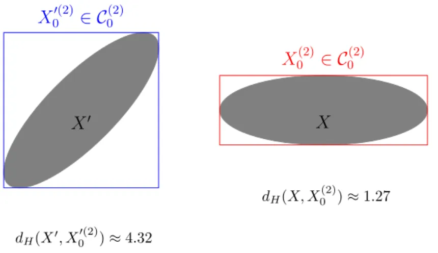
Of course the C₀(N )-approximation is sensitive to rotations (see Figure 1). Obviously, it can be problematic to describe the geometry of sets. Let us con-sider the following example of an ellipse.

X

X

∈ C

X

∈ C

X

Figure 1: The C₀(N )-approximations of an ellipse X and its rotation X0 with respect to the angle π₄.

Example 2.1. Let X be an ellipse with semi-axis a = 1 and b = 3, and suppose that the major semi-axis b is horizontally oriented. Firstly consider the case N = 2, and let us note X0 _{:= Rπ}

4(X), the following Figure 1 shows that the

C0(N )-approximation of X is better than the one of X0 (in terms of the

Haus-dorff ’s distance). Indeed, dH(X, X (2)

0 ) << dH(X0, X 0(2)

0 ). Furthermore, the

C₀(2)-approximation of the rotation is not the rotation of the C₀(2)-approximation. Therefore, it can be problematic to use the C₀(2)-approximation to describe the shape of X. Note that for the ellipse X of Figure 1, the orientations 0 and π₄ are respectively the better and the worst case for the C₀(2)-approximation.

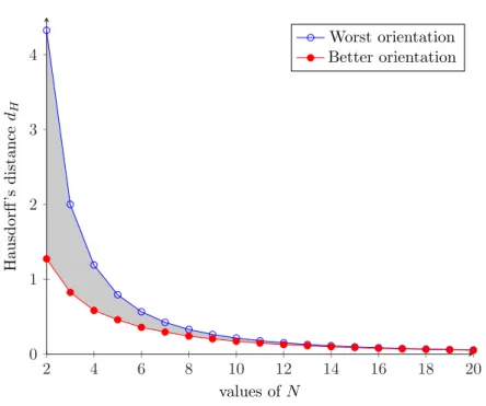
Let us consider now the more general case of the approximation of the rotations of X for different values of N . For each N = 1, · · · 20, the C₀(N ) -approximations of all of the rotations Rη(X) of X has been computed. Among

these approximations, the better ηb and the worst ηw angles (in terms of the

Hausdorff ’s distance) have been retain. The corresponding Hausdorff ’s distances are represented in Figure 2. Consequently, whatever the orientation of the el-lipse, the Hausdorff ’s distance is inside the gray region. It can be noticed, that for small values of N , the difference between the worst and the better case is more important.

For the reasons mentioned above, it can be interesting to have an isometric invariant approximation. Fortunately, for a symmetric convex set X, the bet-ter C₀(N )-approximation (in terms of the Hausdorff’s distance) of the family of rotations of X can be used to define such an isometric invariant approximation.

2 4 6 8 10 12 14 16 18 20 0 1 2 3 4 values of N Hausdorff ’s distance dH Worst orientation Better orientation

Figure 2: The Hausdorff’s distance between an ellipse of semi-axis (1, 3) and its C₀(N )-approximation for several values of N . The case of the better direction in red and worst in blue. The gray region, represent the possible values for this distance.

2.3

Approximation of a symmetric convex set by a regular

zonotope

It has been shown previously how a symmetric convex set X can be approxi-mated in the class of the 0-regular zonotope. Such approximation is sensitive to the rotations. However, in order to study convex sets, there is sometime a need to have isometric invariant tools. Therefore, it will be defined here an approximation which is invariant up to a rotation. To meet this gool there is a need to perform the approximation on a class larger than C(N )₀ , namely the class of the regular zonotopes.

Definition 2.4 (t-regular and regular zonotopes). Let t ∈ R and N > 1 be an integer, C_t(N ) denotes the class of the rotated elements of C₀(N ) with respect to the angle t:

C_t(N )= {Rt(X)|X ∈ C (N ) 0 }

Any element of C_t(N ) is called a t-regular zonotope with 2N faces.

Furthermore, C(N )∞ = S_t∈RCt(N ) denotes the set of the regular zonotopes with

2N faces.

All the properties of C₀(N ) cited above are also true for C_t(N )_{, t ∈ R.} There-fore, it will be defined an approximation in C(N )∞ .

Theorem 2.2 (Approximation in C∞(N )). Let X ∈ C and let us note X0N(t)

the C₀(N )-approximation of R−t(X).

i. There exists τ ∈ [0, π[ satisfying:

dH(Rτ(X0N(τ )), X) = dH(X0N(τ ), R−τ(X)) = min t∈RdH(X N 0 (t), R−t(X)) (17) XN

0 (τ ), also denoted ˜X0N, will be named the C (N )

0 -rotational approximation

of X.

ii. The C₀(N )-rotational approximation of X is invariant under rotations of X.

The set Rτ(X0N(τ )) will be called a C∞N-approximation of X in C (N )

∞ and will be

denoted by X∞(N ).

Proof.

1. First of all, because of the symmetry of the 0-regular zonotopes: ∀t ∈ R, Ct(N )= C

(N )

t+π⇒ mint∈RdH(X0N(t), R−t(X)) = mint∈[0,π]dH(X0N(t), R−t(X)).

For any t ∈ R, let us note α(t) the face length vector of X0N(t) then for

any h ∈ R : k α(t) − α(t + h) k₁=k F(N )−1(H_R(N ) −t(X)− H (N ) R−t−h(X)) k1 ⇒ k α(t) − α(t + h) k₁≤k F(N )−1_k 1k H (N ) R−t(X)− H (N ) R−t−h(X)k1

However, ∀η ∈ R, HR−t−h(X)(η) = HR−t(X)(η + h) . Because of the

continuity of the Feret’s diameter k H_R(N )

−t(X)− H

(N )

R−t−h(X)k1→ 0 as h → 0

then k α(t) − α(t + h) k₁→ 0 as → 0.

Therefore from the expression(7) about the Feret’s diameter of a zonotope, ∀η ∈ R,: |H_XN 0(t+h)(η) − HX0N(t)(η)| =|( N X i=1 (αi(t) − αi(t + h))| sin(η − θi)|)| ≤ N max i=1,···N{(αi(t) − αi(t + h))} then |H_XN 0 (t+h)(η)−HX0N(t)(η)| → 0 as h → 0 and finally dH(X N 0 (t), X0N(t+

h)) → 0 as h → 0. Consequently, the map t 7→ XN

0 (t) is continuous with

respect to the Hausdorff’s distance.

Note that ∀x ∈ R, HRt(X0N(t))(x) = HX0N(t)(x−t) and HX(x) = HR−t(X)(x−

t) then: HRt(X0N(t))(x) − HX(x) = HXN0(t)(x − t) − HR−t(X)(x − t) ⇒dH(Rt(X0N(t)), X) = dH(X0N(t), R−t(X)) ⇒ min t∈RdH(Rt(X N 0 (t)), X) = min t∈RdH(X N 0 (t), R−t(X))

Furthermore for any x, h ∈ R, |H_Rt(XN

...H_XN 0 (t+h)(x − t) + HX N 0(t+h)(x − t) − HX N 0 (t+h)(x − t − h)| ≤ |H_XN 0 (t)(x − t) − HX0N(t+h)(x − t)|... ... + |HXN 0(t+h)(x − t) − HX0N(t+h)(x − t − h)|

then from the continuity of the Feret’s diameter and of the map t 7→ XN(t),

it follows the continuity of t 7→ Rt(X0N(t)). As a consequence the map t 7→

dH(X0N(t), X) is also continous and the minimum mint∈[0,π]dH(Rt(X0N(t)), X)

is achieved. Then there is a ∈ [0, π] such that dH(Rτ(X0N(τ )), X) =

min_t∈RdH(X0N(t), R−t(X)).

2. Let us prove the invariance by rotations. Let η ∈ [0, π] and Y = Rη(X),

then YN 0 (t) is the C (N ) 0 -approximation of R−(t−η)(X) and Y0N(t) = X0N(t− η). Furthermore, min t∈RdH(Y N 0 (t), R−t(Y )) = min t∈RdH(X N 0 (t − η), R−(t−η)(X)) = min t∈RdH(X N 0 (t), R−(t)(X)) = dH(X0N(τ ), R−τ(X)) Then XN 0 (τ ) is a C (N )

0 -rotational approximation of Y and the C (N )

∞ -approximation

associated is Rη(Rτ(X0N(τ ))) (indeed Y0N(τ + η) = X0N(τ )).

The proposition above gives important informations. The C∞(N )-approximation

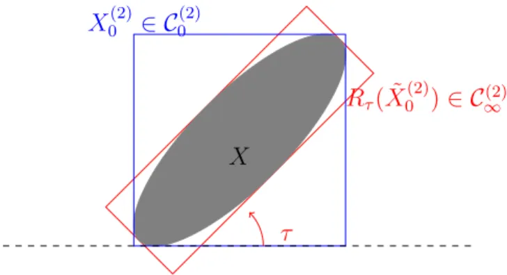
of a symmetric convex set X is the best regular zonotope with at most 2N faces containing X. It is always a better approximation than the C₀(N )-approximation. This approximation can be used for not so large N . For example, for N = 2, the C₀(2)-approximation of an ellipse depends on the orientation of the ellipse, but its C∞(2)-approximation is the best way to put the ellipse inside a rectangle

(see Figure 3). An illustration of the approximations of that ellipse for higher value of of N is representedFigure 4.

X

X

∈ C

R

( ˜

X

) ∈ C

τ

Figure 3: An ellipse and its approximations: X2∈ C (2)

0 in blue and Rτ( ˜X2) ∈

C₀(N )-approximations

X

X

Figure 4: The C₀(N )-approximations(left) and C(N )∞ -approximations(right) of an

ellipse of semi-axis (3, 1) for different values of N (= 3, 4, 10).

The accuracy of the C(N )₀ -approximation has been presented inFigure 2and one can remark that the best orientation corresponds to the C∞(N )-approximation.

Then, for the considered ellipse, the accuracy of the C∞(N )-approximation in

function of the number of faces N has already been represented in Figure 2. However, the accuracy of the C∞(N )-approximation depends both on the shape

and the size of the symmetric convex X.

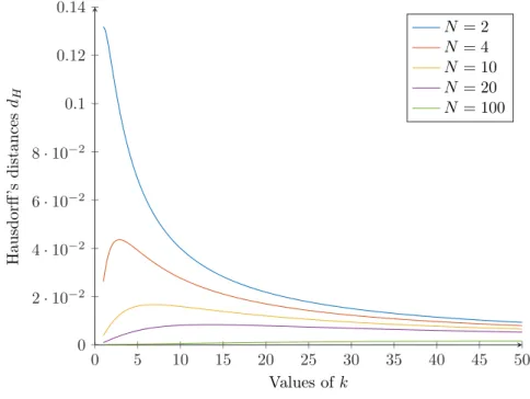
0 5 10 15 20 25 30 35 40 45 50 0 2 · 10−2 4 · 10−2 6 · 10−2 8 · 10−2 0.1 0.12 0.14 Values of k Hausdorff ’s distances dH N = 2 N = 4 N = 10 N = 20 N = 100

Figure 5: The Hausdorff’s distance between an ellipse of unit perimeter and its C∞(N )-approximations for several values of N in function of its axis ratio k.

Remark 2.4 (Accuracy of the C∞(N )-approximation). The size dependence

of the accuracy is easy to understand: the accuracy decreases proportionally to the size factor. Indeed, for Y := kX, k ∈ R+ we have dH(Y

(N ) ∞ , Y ) =

kdH(X (N )

∞ , X) (because of the homogeneity of the Feret’s diameter). In order

to study the impact of the shape (independently of its size) on the approxima-tion accuracy, there is a need to use an homothetic invariant descriptor. In order to do this, the Feret’s diameter of a symmetric convex set X will be nor-malized by its perimeter. According to Cauchy’s formula [27] the perimeter is equal to the Feret’s diameter total mass Rπ

0 HX(θ)dθ. Then, according to

the homogeneity of the Feret’s diameter, an involved distance can be defined as ∀X, Y ∈ C, ˜dH(X, Y ) := dH(_{U (X)}X ,_{U (Y )}Y ). Such a distance can be used to study

the approximation accuracy. Notice that it is equivalent to work with sets of unit perimeters and using the usual Hausdorff ’s distance. Such a consideration will be done in the following example.

Let us consider an ellipse X with unit perimeter and an axis ratio k ∈ [1, +∞[, the case k = 1 referring to the disk. The accuracy of the C∞(N )

-approximation as a function of N and k is shown. More specifically, on the Figure 5 it can be seen that the behaviour of the curves are very different for different values of N . Indeed, the worst shape for N = 2 is the disk. However, as it can be seen that is not the case for others values of N . It can be noticed that when the ratio k increases, the importance of N for the approximation de-creases. This suggests that when an object X is elongated, one can choose a small value of N .

It has been studied two different approximations of a symmetric convex set X. The first one is an approximation of X as 0-regular zonotope, and the second as a regular zonotope. These approximations have been characterized from the Feret’s diameter of X. The next objective is to study these approximations when X become a random symmetric body, and then how they can be characterized from the Feret’s diameter of X. In order to do this, there is a need to study some properties of the random zonotopes, which lead us to the following section.

3

The random zonotopes

The aim of this section is to investigate how a random zonotope can be described by a random vector representing its faces and how such random vector can be characterized from the Feret’s diameter of the random zonotope. Firstly, the properties of the random process corresponding to the Feret’s diameter of a random set, will be investigated. In a second time, the description of a random zonotope by its faces will be explored. Finally, the characterization of some random zonotopes from their Feret’s diameter random process will be given.

3.1

Feret’s diameter process and isotropic random set

Let X be a random convex set, i.e a random closed set which is almost surely a convex set. In this subsection, some properties of the random process [9] corresponding to the Feret’s diameter of X are stated.

Definition 3.1 (Feret’s diameter random process). Let X be a random convex set of R2

. For all ω ∈ Ω a.s X(ω) is a convex set. Then, for any t ∈ R, the positive random variable HX(t) : ω 7→ HX(ω)(t) is almost surely defined.

The random process {HX(t), t ∈ R} will be named the Feret’s diameter random

process of X.

The trajectories of HX are the Feret’s diameter of the realizations of X,

then the properties of the proposition 2.2 are also true for these trajectories, especially the continuity and the π-periodicity. It can be also noticed that the Feret’s diameter random process characterizes the symmetric convex sets.

Definition 3.2 (Isotropised set of a random symmetric body). Let X0 be a symmetric random convex set and let η be a random uniform variable on [0, π] independent of X0, the set

X := Rη(X0)

is isotropic (a random compact is said to be isotropic if and only if its distri-bution is isometric invariant [8]) and will be called an isotropised set of X0.

Let X0 be a random symmetric body and X be an isotropised set of it, then X and X0 have the same shape distribution and they also have the same zono-tope rotational approximations (see theorem2.2).

In the following, it will be shown that the Feret’s diameter random process HX0

of X0 can be expressed from the one of X. This property will be used to show that a random symmetric convex set can be described up to a rotation by an isotropic random zonotope.

Let us recall that the Feret’s diameter random process HX0 of X0 is enough

to characterize X0_{, then for any θ ∈ R the Feret’s diameter H}X0 of X0 can be

expressed as:

HX(θ) = HX0(θ − η)

Let B be a Borel subset of R. Because of the uniformity of η and its indepen-dence with X0, it follows:

P(HX(θ) ∈ B) = P(HX0(θ − η) ∈ B) = 1 2π Z 2π 0 P(HX0(θ − t) ∈ B)dt

Furthermore, by using the π-periodicity of the Feret’s diameter, the distribution of HX(θ) can be expressed as:

P(HX(θ) ∈ B) = 1 π Z π 0 P(HX0(θ − t) ∈ B)dt (18)

Consequently, the moments of the Feret’s diameter process of the set X0_{and the}

isotropised set X are related. Of course there is a need to ensure their existence, but it will be treated after.

Proposition 3.1 (Moments of the Feret’s diameter process of the isotropised set). Let X0 be a random convex set and X the isotropised set of X0. Suppose that the first and second order moments of the Feret’s diame-ter random process HX0 of X0 exists, then those of X exists and they can be

expressed as: ∀θ ∈ [0, 2π], E[HX(θ)] = 1 π Z π 0 E[HX0(θ)]dθ ∀(s, t) ∈ [0, 2π]2 , E[HX(s)HX(t)] = 1 π Z π 0 E[HX0(θ)H_X0(θ + s − t)]dθ

Proof. Let X0 be a random convex set and X = Rη(X0) an isotropised set of

it and suppose that first and second order moments of HX0 exist. Let us recall

that ∀θ ∈ R, HX(θ) = HX0(θ − η) and that η is independent of X0 thus the

result comes by integrating with respect to the uniform distribution of η. Proposition 3.2 (Feret’s diameter process of an isotropic random con-vex set). Let X0 be a random convex set.

i. If X0 is isotropic then the random variables HX0(θ), θ ∈ [0, π] are

identi-cally distributed (i.e the random process HX0 is stationary).

ii. Furthermore, if X0 is symmetric the reciprocal is true.

Proof.

1. Let η be a uniform random variable on [0, π] independent of X0 and let note X = Rη(X0). If X0 is isotropic then X and X0 have the same

distri-bution then HX and HX0 have also the same distribution. Consequently,

according to (18), for any θ ∈ [0, π] and for any borel set B,

P(HX0(θ) ∈ B) = P(H_X(θ) ∈ B) = 1 π Z π 0 P(HX0(θ − t) ∈ B)dt

Because of the π-periodicity of the Feret’s diameter, the integral is un-dependable of θ and thus the random variables HX0(θ), θ ∈ [0, π] are

identically distributed.

2. Suppose that X0 is symmetric and HX0(θ), θ ∈ [0, π] are identically

dis-tributed. Then the random process HX0 is stationary, that is to say: for

any x ∈ R, the random process (HX0(θ))_θ∈R and the translated process

( ˜HX0(θ) = H_X0(θ + x))_θ∈R have the same distribution. However ˜H_X0

is exactly the random process corresponding to the Feret’s diameter of Rx(X0). It has been already established that the Feret’s diameter

char-acterizes the symmetric bodies, then for any x ∈ R, Rx(X0) and X0 have

the same distribution, so X0 _{is isotropic.}

It has been shown some properties of the Feret’s diameter random process. Let us discuss now about the random zonotopes, that is to say the random sets almost surely valued in C(N )_.

3.2

Description of the random zonotopes from their faces

Here it will be defined some classes of random zonotopes. Particularly, the class of the random zonotopes almost surely valued in C₀(N ) and the class of those almost surely valued in C(N )∞ . Several properties of the random zonotopes will

be studied. In particular, it will be shown how a random zonotope can be described by a random vector corresponding to its faces.

Definition 3.3 (Random zonotopes). Let N > 1 be an integer, a random closed set X which has almost surely its realizations in C(N ) will be called a random zonotope with at most 2N faces or, in a more concise way, a random zonotope when there is no possible confusion.

Such a random set can be described almost surely as:

∀ω ∈ Ω a.s , X(ω) =

N

M

i=1

αi(ω)Sβi(ω)

The distribution of the random vector (α, β) characterizes X. The random vector α will be named a face length vector of X.

According to proposition2.3, for any face length vector α of X, some geometrical characteristics (Feret’s diameter, perimeter, area) of X can be expressed as:

∀ω ∈ Ω a.s , ∀t ∈ R, HX(t) = N X i=1 αi| sin(t − βi)| (19) ∀ω ∈ Ω a.s , U (X) = 2 N X i=1 αi (20) ∀ω ∈ Ω a.s , A(X) = 1 2 N X i=1 N X j=1 αiαj| sin(βi− βj)| (21)

Proposition 3.3 (Existence conditions for the auto-covariance of the Feret’s diameter process). Let X be a random zonotope with 2N faces and α its face length vector, then the following properties are equivalent:

E[U (X)2] < ∞ (22) α ∈ L2_(RN+) (23)

Furthermore, if one of these conditions is satisfied then E[A(X)] < ∞ and ∀(s, t) ∈ [0, π]2

, E[HX(s)HX(t)] < ∞.

Proof. According to (20), U (X)2_{= (2}PN

i=1αi)2, the first equivalence is trivial

(because of the positivity of α).

The proposition2.3 also shows that: ∀(s, t) ∈ [0, π]2_,

HX(s)HX(t0) = N X i=1 N X j=1 αiαj| sin(s − η − βi) sin(t − η − βi)| ≤ N X i=1 N X j=1 αiαj

≤1 4U (X)

2

Then the expectation E[HX(s)HX(t)] exists and the existence of E[A(X)] comes

from the isoperimetric inequality.

Definition 3.4 (0-regular random zonotopes). Let N > 1 be an integer, a random closed set X which has almost surely its realizations in C₀(N ) will be called a 0-regular random zonotope with at most 2N faces or, in a more concise way, a 0-regular random zonotope when there is no possible confusion.

A 0-regular random zonotope X can be almost surely expressed as:

∀ω ∈ Ω a.s , X(ω) =

N

M

i=1

αi(ω)Sθi

where θi, i = 1, · · · N denotes the regular subdivision on [0, π].

The distribution of the face length vector α characterizes the distribution of X. In addition, this relation is bijective; in other word, the α’s distribution is uniquely defined, it will be named the face length distribution.

Of course the 0-regular random zonotopes can be used to approximate the random symmetric convex sets as N → ∞ (see section4.1). However, it is not the best way to model a random symmetric convex set. Indeed, it can be noticed that a 0-regular random zonotope cannot be isotropic. For instance, there is a need to use a large N in order to describe a random set built as an isotropic random square (see example4.1). That is the raison for using a larger class of random zonotopes.

Definition 3.5 (Regular random zonotopes). Let N > 1 be an integer, any random compact set taking its value almost surely in C∞(N ) will be named a

regular random zonotope and can be expressed as:

X = Rx( N

M

i=1

αiSθi)

where x is a random variable on [0, π] and α a random vector taking values in RN+. The random vector α will be named a random face length vector of X.

Proposition 3.4 (Isotropic regular random zonotope). Let X = Rx(LNi=1αiSθi)

be an isotropic regular random zonotope, then X has the same distribution of the following random set:

X a.s= Rη( N

M

i=1

αiSθi) (24)

where η is a uniform random variable on [0, π] independent of α.

Proof. Let X = Rx(LNi=1αiSθi) be an isotropic regular random zonotope, and

η0be a uniform random variable independent of α. Because of the isotropy of X, the random set Rη0(X) has the same distribution as X. Let η = x + η0[π] then

the random set Rη0(X) can be expressed as R_η(LN_i=1α_iS_θ

i). Consequently,

Rη(LNi=1αiSθi) has the same distribution as X.

Let us show that η is a uniform variable independent of α.

Let B be a Borel set of RN _{and for all t ∈ [0, π], E denotes the event E = {η ∈}

[0, t]} ∩ {α ∈ B} then: E = {α ∈ B} ∩ ( [ z∈[0,π] {x = z} ∩ {η0+ z[π] ≤ t}) = [ z∈[0,π] {α ∈ B}{x = z} ∩ {η0+ z[π] ≤ t}

Note that this union is disjointed, then because of the independence of η0:

P(E) = Z π

0

P({α ∈ B}{x = z})P({η0+ z[π] ≤ t})dz

The quantity P({η0_{+ z[π] ≤ t}) is independent of the value of z and it can be}

easily computed as P({η0+ z[π] ≤ t}) = t π. Consequently: P(E) = t π Z π 0 P({α ∈ B}{x = z})P({η0+ z[π] ≤ t})dz P(E) = t πP({α ∈ B})

then η is a uniform random variable on [0, π] independent of α.

The proposition above shows that an isotropic regular random zonotope can always be described as (24). Such a zonotope is consequently defined by its random face length vector α. However, different distributions of α can lead to the same distribution of X as mentioned in the following proposition.

Proposition 3.5 (Family of the random face length vectors). Let α be a random face length vector of the isotropic regular random zonotope X. The following family of random face length vectors, denoted FN(X), provides the

same distribution of the random set X:

FN(X) = {α0 a.s= Jnα|∀ω ∈ Ω a.s , n(ω) ∈ {0 · · · , N − 1}} (25)

where J is the circulant matrix J = Circ(0, 1, 0, · · · 0).

Proof. First of all, it is easy to see that FN(X) is not empty by construction of

X. Let α, α0 be two representative random vectors of X then there exists two uniform random variables η and η0 satisfying η ⊥⊥ α and η0_{⊥⊥ α}0 _{such that :}

∀ω ∈ Ω a.s , N M i=1 αi(ω)Sθi+η(ω)= M M i=1 α0_i(ω)Sθi+η0(ω) ⇒∀ω ∈ Ω a.s , R−η0_(ω)( N M i=1 αi(ω)Sθi+η(ω)) = R−η0(ω)( N M i=1 α0i(ω)Sθi+η0(ω)) ⇒∀ω ∈ Ω a.s , N M i=1 α0_i(ω)Sθi = N M i=1 αi(ω)Sθi+η(ω)−η0(ω)

Then, because of the uniqueness of the face length vector in C₀(N ), for any ω ∈ Ω a.s there is j(ω) ∈ {1, · · · N } such that:

θ1= (θj(ω)+ η(ω) − η0(ω))[π] and α10(ω) = αj(ω)

⇒ θj(ω)= (η0(ω) − η(ω))[π] and α01(ω) = αj(ω)

⇒ α0

i(ω) = αi+j−1[M ](ω)

⇒ α0(ω) = Jj(ω)−1α(ω)

By taking ∀ω ∈ Ω a.s , n(ω) = j(ω)−1[N ] it follows α0= Jn_{α and consequently}

FN(X) ⊂ {α0 = Jnα|∀ω ∈ Ω a.s , n(ω) ∈ {0 · · · , N − 1}}.

The other inclusion can be proved by taking η0 such that ∀ω ∈ Ω a.s , η0(ω) = βn(ω)+1+η[π]. For such an η0it follows ∀ω ∈ Ω a.s , X(ω) =L

N

i=1α0i(ω)Sθi+η0(ω).

Definition 3.6 (Central random face length vector). Let α ∈ FN(X) and

n be a uniform random variable on {0 · · · , M − 1} independent of α, then the random face length vector α0= Jn_{α will be called a central random face length}

vector of X.

Notice that a central random face length vector has all of these components identically distributed. Furthermore, its distribution has many interesting prop-erties.

Proposition 3.6 (Uniqueness of the central face length distribution). There is a unique distribution for any central random face length vectors. In other words, let ˜α0, α0 be two central random face length vectors of X, then they have same distribution. Such a distribution will be named the central face length distribution of X.

Proof. Let ˜α0 and α0 be two central representations of X. Then there ex-ists a random face length vector ˜α and an independent uniform variable ˜n on {0 · · · , N − 1} such that ˜α0 = Jn˜_{α. In addition, ˜˜ α ∈ F}

N(X) so there exists n

such that ˜α = Jn_α0_{. Consequently ˜α}0 _{= J}n+n˜ _α0_{. Let n}0 _{= ˜n + n[N ], it is easy}

to see that J˜n+n_{= J}n0_{, thus:}

˜

α0= Jn0α0

Let us prove that n0 is a uniform variable on {0 · · · , M − 1} independent of α0. For any k ∈ {0 · · · , N − 1}, P({n0= k}) = P( N −1 [ i=0 {˜n = k − i[N ]} ∩ {n = i}) = N −1 X i=0 P({˜n = k − i[N ]})P({n = i}) = 1 N

then n0 _{is a uniform variable on {0 · · · , N − 1}. Furthermore for any Borel set}

B and any k ∈ {0 · · · , N − 1} : P({n0= k} ∩ {α0∈ B}) = P( N −1 [ i=0 {˜n = k − i[N ]} ∩ {n = i} ∩ {α0∈ B})

= N −1 X i=0 P({˜n = k − i[N ]} ∩ {n = i} ∩ {α0 ∈ B}) = N −1 X i=0 P({˜n = k − i[N ]})P({n = i} ∩ {α0∈ B}) = 1 N N −1 X i=0 P({n = i} ∩ {α0∈ B}) = 1 NP({α 0_{∈ B})} = P({n0= k})P({α0 ∈ B})

Now let us prove that α0 and ˜α0 have the same distribution. Let B = B0×

· · · × BN −1 a product of Borel sets of R. Firstly, note that ∀k ∈ {0 · · · , N −

1}, P(Jk_α0 _{∈ B) = P(α}0 _{∈ B). Indeed, by definition, α}0 _{can be written as}

α0= Jn_{α with α a representative of X and n an independent uniform random}

variable on {0 · · · , N − 1}. Therefore, P({α0∈ B}) = P( N −1 [ i=0 {Ji_{α ∈ B} ∩ {n = i})} = 1 N N −1 X i=0 P({Jiα ∈ B}) = 1 N N −1 X i=0 P({α ∈ Bi× · · · B0· · · BN −1−i})

In the same manner,

P({Jkα0∈ B}) = 1 N N −1 X i=0 P({Ji+kα ∈ B}) = 1 N N −1 X i=0 P({α ∈ Bi+k× · · · B0· · · BN −1−i−k}) = 1 N N −1 X i=0 P({α ∈ Bi× · · · B0· · · BN −1−i}) = P({α0∈ B}) Furthermore, P({ ˜α0 ∈ B}) = P( N −1 [ k=0 {Jk_α0_{∈ B} ∩ {n}0_{= k})} = 1 N N −1 X k=0 P({Jkα0 ∈ B}) = P({α0∈ B})

Proposition 3.7. [Properties of the central face length distribution] Let α be a central random face length vector of X, then the first and second order moments of its distribution have the following properties:

i. first order moment:

∀i = 1, · · · N, E[αi] =

U (X)

2N (26)

ii. second order moment:

The matrix C[α] = (E[αiαj])1≤i,j≤N is a circulant matrix defined by the

first column V [α] =t _(E[α1α1], · · · E[α1αN]): C[α] = Circ(V [α]).

Fur-thermore this matrix is symmetric, it depends only on (bN₂c + 1) val-ues, where bN₂c denotes the floor of N

2. Let us note m = b N

2c and

v =t

(E[α1α1], · · · E[α1αm+1]) therefore if N is an even integer V =t

(v0, · · · vm−1, vm, vm−1, · · · v1) and if N is an odd integer V =t(v0, · · · vm, vm, · · · v1).

Proof.

1. The first point is trivial. Indeed the marginals of α are identically dis-tributed then ∀i, j E[αi] = E[αj] and U (X) = 2PNi=1αi⇒ ∀i = 1, · · · N, E[αi] = U (X)

2N .

2. It has been shown that for any k ∈ {0 · · · , N − 1}, the random variables α and Jk_{α have same distribution, then they have the same covariance}

matrix. Therefore ∀1 ≤ i, j ≤ N :

∀k ∈ {0 · · · , N − 1}, E[αiαj] = E[αi+k[N ]+1αj+k[N ]+1]

so E[αiαj] is a circulant matrix, it depends only on i − j[N ] and because

of its symmetry also only on j − i[N ]. Let 1 ≤ i ≤ j ≤ N then there is two possible case , first suppose that N = 2m is an even integer, then ∀0 ≤ k ≤ m − 1 :

E[α1α1+m+k] = E[α1+mα1+k] = E[α1+m+N −kα1+N] = E[α1α1+m−k]

then by noting V =t_(E[α1α1], · · · E[α1αN]) and v =t(E[α1α1], · · · E[α1αm+1])

there is V =t(v0, · · · vm−1, vm, vm−1, · · · v1).

If N is an odd integer, then N = 2m + 1 and for any 0 ≤ k ≤ m: E[α1α1+m+k] = E[α1+m+1α1+k] = E[α2+m+N −kα1+N] = E[α1α2+m−k]

then by noting V [α] =t

(E[α1α1], · · · E[α1αN]) and v =t(E[α1α1], · · · E[α1αm+1])

there is V =t_(v

0, · · · vm, vm, · · · v1). Finally C[α] is a symmetric circulant

matrix.

Example 3.1. In order to illustrate the properties of the face length vector dis-tributions, let us discuss about the case N = 2. Then, X = Rη(α1S0⊕ α2Sπ

2)

Therefore X is an isotropic random rectangle described by its sides (α1, α2).

However, that is not the unique way to describe it. Indeed, even for a deter-mistic rectangle of sides (a, b) it can also be said that its sides is (b, a). This simple fact involves a lot of different distributions for the face length vectors of an isotropic random rectangle.

Let us take this simple example: suppose Y is equiprobably the rectangle of sides (1, 2) or the rectangle of sides (3, 4). Then, there is at least the following four possible descriptions for the sides of Y ’s realization:

• (1, 2) or (3, 4) • (2, 1) or (3, 4) • (2, 1) or (4, 3) • (1, 2) or (4, 3)

Therefore, there are four corresponding face length distributions 1₂∆(1,2)+12∆(3,4), 1

2∆(2,1)+ 1

2∆(3,4),... where ∆(a,b)denotes the Dirac measure in (a, b). However,

there are not the only possibilities. Indeed, many other can be built from the previous distributions, such as the distribution 1₄∆(1,2)+14∆(2,1)+12∆(3,4).

No-tice that the central distribution of Y is 1₄∆(1,2)+1₄∆(2,1)+1₄∆(3,4)+1₄∆(4,3).

Let us return now to the general case of the isotropic random rectangle X with a face length vector α. According to the foregoing, it is easy to see that any another face length vector α0 of X can be built as :

α0 =Å1 − δ δ δ 1 − δ

ã

α (27)

where δ is any Bernoulli variable (i.e valued in {0, 1}) eventually correlated to α.

Indeed, it should be noticed that Å1 − δ δ δ 1 − δ ã = Jδ_{, therefore by taking} η0 = η + δπ₂[π], X = Rη(α1S0⊕ α2Sπ 2) = Rη0(α 0 1S0⊕ α02Sπ₂)

it can be easily proved that η0 is a uniform random variable on [0, π] independent of α0 (see proof of proposition 3.6), then α0 is a face length vector of X.

Let us consider now the central face length distribution, so let δ be a Bernoulli variable of parameter 1₂ (i.e a uniform variable on {0, 1}) independ of α, and let α0= Jδα be a central face length vector, then acording to (27),

α0₁= (1 − δ)α1+ δα2

α0₂= δα1+ (1 − δ)α2

Consequently, the first and second order moments of the face length distri-bution can be computed as:

E[α01] = E[α02] =

1

E[α01 2 ] = E[α02 2 ] =1 2E[α 2 1+ α22] E[α01α 0 2] = E[α1α2]

Notice that the property3.7_{is well verified,. Indeed, E[α}0_{1] = E[α}0₂] = 1

4E[U (X)]

and the matrix C[α] is a circulant matrix depending on two parameters.

3.3

Characterizing an isotropic regular random zonotope

from its Feret’s diameter random process

It has been shown that the distribution of an isotropic random zonotope X can be described by its central face length distribution. The properties of such distributions have been studies. Here it will be shown how its characteristics can be connected to the geometrical characteristics of the random zonotope. In particular, it will be given formulae which allows to connect the first and sec-ond order moments of Feret’s diameter of X to whose of the central face length distribution.

Let X be an isotropic random zonotope represented by its face length vector α. Let us recall that X can be almost surely expressed as:

X = Rη( N

M

i=1

αiSθi)

where η is a uniform random variable independent of α ≥ 0. Suppose that the condition E(U (X)2_{) < ∞ is satisfied, then according to the proposition 3.3,}

α ∈ L2

(RN

+) and the mean and the auto-covariance of HX exist.

According to the proposition2.3, for any representative α of X, some geo-metrical characteristics of X can be expressed as:

∀t ∈ R, HX(t) = N X i=1 αi| sin(t − η − θi)| U (X) = 2 N X i=1 αi A(X) = 1 2 N X i=1 N X j=1 αiαj| sin(θi− θj)| Thefore, by considering α ∈ L2 (RN

+) and the independence of α and η, their

expectation can be computed by integration with respect to the uniform distri-bution of η: ∀t ∈ R, E[HX(t)] = 2 π N X i=1 E[αi] (28) E[U (X)] = 2 N X i=1 E[αi] (29)

A(X) = 1 2 N X i=1 N X j=1 E[αiαj]| sin(θi− θj)| (30) ∀t, t0∈ R, E[HX(t)HX(t + t0)] = N X i=1 N X j=1 E[αiαj]kS(t0+ θi− θj) (31) where ∀t ∈ R, kS(t) = 1 π Z π 0 | sin(t + z) sin(z)|dz (32) Note that kS is a π-periodic function and it can be expressed on [0, π] as:

kS(t) =

1 2π(2 sin

3_{(t) + cos(t)(π − 2t + sin(2t))) (33)}

By using the equation (31) and the stationarity of HX:

∀t, t0∈ R, E[HX(t)HX(t + t0)] = E[HX(t)HX(t − t0)] (34) ∀t, t0∈ R, N X i=1 N X j=1 E[αiαj]kS(t0+ θi− θj) = N X j=1 N X i=1 E[αiαj]kS(t0+ θj− θi) (35) and by introducing the following functional:

∀t ∈ R, ∀1 ≤ i, j ≤ N, Kij(t) = kS(t + θi− θj) (36) it follows: ∀t, t0 ∈ R, E[HX(t)HX(t + t0)] = N X i=1 N X j=1 E[αiαj]Kij(t0) (37)

Proposition 3.8. For any real t, K(t) is a circulant matrix. Furthermore, by

denoting ((k1(t), · · · kN(t))) the first line of K(t), we have K(t) = Circ((k1(t), · · · kN(t)))

and Kij(t) = kj(θi+ t) for 1 ≤ i, j ≤ N .

Proof. Let us show that K(t) is a circulant matrix. For any real t, t + θi− θj

depends only on i − j then K(t) is a Toeplitz matrix. Furthermore for 1 ≤ i ≤ N − 1 and 1 ≤ j ≤ N, K(i+1)j(t) = kS(t + θi− (θj−_Nπ)) but (θj−_Nπ) = θσ(j)

where σ(j) = (j − 2[N ]) + 1, then K(i+1)j(t) = Kiσ(j). Therefore, the line index

i + 1 of K(t) is a cyclic permutation of the line index i of K(t) so K(t) is a circulant matrix. Furthermore kj(θi+ t) = kS(t + θi− θj) = Kij(t).

Suppose now that α is a central representative of X, it will be shown that the first and second order moments of the central distribution can be easily expressed from the Feret’s diameter process.

Theorem 3.1 (Moments of the central face length distribution). Let X be an isotropic random zonotope represented by a central face length vector α, then: ∀x ∈ R, ∀i = 1, · · · N, E[αi] = π 2NE[HX(x)] (38) V [α] = 1 NK(0) −1_{V [H}(N ) X ] (39)

where V [x] denotes the vectort

Proof. Suppose that α is a central representative of X, then according to the propositions 3.7 and the equation (28) the first order moment of the central distribution can be expressed as:

∀x ∈ R, ∀i = 1, · · · N, E[αi] =

π

2NE[HX(x)] (40) Considering the propositions3.8 and3.7_{, it comes E[α}iαj] = V [α]j−i[N ]+1 and

Kij(t) = kj−i[N ]+1then for all t ∈ R,

E[HX(0)HX(t)] = N X i=1 N X j=1 E[αiαj]Kij(t) = N X i=1 N X j=1 V [α]j−i[N ]+1kj−i[N ]+1(t) = N X i=1 i X j=1 V [α]j−i[N ]+1kj−i[N ]+1(t) + N X i=1 N X j=i V [α]j−i[N ]+1kj−i[N ]+1(t) − N X i=1 V [α]1k1(t) = N X i=1 i−1 X s=0 V [α]s+1ks+1(t) + N X i=1 N −i X s=0 V [α]s+1kN −s[N ]+1(t) − N V [α]1s1(t) = N X i=1 i−1 X s=0 V [α]s+1ks+1(t) + N X i=1 i X z=N V [α]N −z+1kz[N ]+1(t) − N V [α]1k1(t) = N X i=1 i−1 X s=0 V [α]s+1ks+1(t) + N X i=1 i X z=N V [α]z[N ]+1kz[N ]+1(t) − N V [α]1k1(t) = N X i=1 i−1 X s=0 V [α]s+1ks+1(t) + N X i=1 N X s=i V [α]s[N ]+1ks[N ]+1(t) − N V [α]1k1(t) = N X i=1 i−1 X s=0 V [α]s+1ks+1(t) + N X i=1 N X s=i V [α]s[N ]+1ks[N ]+1(t) − N V [α]1k1(t) = N X i=1 N X s=0 V [α]s[N ]+1ks[N ]+1(t) − N V [α]1k1(t) = N X i=1 N −1 X s=0 V [α]s[N ]+1ks[N ]+1(t) + N X i=1 V [α]1k1(t) − N V [α]1k1(t) = N X i=1 N −1 X s=0 V [α]s+1ks+1(t) = N X i=1 N X s=1 V [α]sks(t)

⇒ E[HX(0)HX(t)] = N N X s=1 V [α]sks(t) (41) Let us note V [H_X(N )] =t

(E[HX(0)HX(θ1)], · · · E[HX(0)HX(θN)]). For 1 ≤ i ≤

N , V [H_X(N )]i= NPNs=1V [α]sks(θi) = NPNs=1V [α]sKis(0) then,

V [H_X(N )] = N K(0)V [α] (42) It is easy to see that K(0) is a symmetric positive definite matrix. Indeed, for 1 ≤ i, j ≤ N, Kij(0) = kS(θi− θj) = kS(θj − θi) = Kji(0) then K(0) is a

symmetric matrix, furthermore ∀x ∈ RN_,

t_{xK(0)x =} N X i=1 N X j=1 xixjKij(0) = N X i=1 N X j=1 xixj 1 π Z π 0 | sin(θi− θj+ z) sin(z)|dz = 1 π Z π 0 N X i=1 N X j=1 xixj| sin(z − θi) sin(z − θj)|dz = 1 π Z π 0 ( N X i=1 xi| sin(z − θi)|)2dz

By denoting Y the following real valued random variable Y =PN

i=1xi| sin(z −

θi)| where z is a uniform random variable on [0, π], then txK(0)x = E[Y2] so t_{xK(0)x ≥ 0. Furthermore} t_{xK(0)x = 0 if and only if Y = 0 almost surely,}

Y = 0 a.s ⇒ ∀z ∈ [0, π], PN

i=1xi| sin(z − θi)| = 0 ⇒ x = 0. Finally K(0) is a

symmetric positive definite matrix, then it is invertible, and it follows: V [α] = 1

NK(0)

−1_{V [H}(N ) X ]

This theorem gives the 1st_{and 2}nd_{order moments of the central face length}

distribution from those of the Feret’s diameter. Note that V [α] and V [H_X(N )] satisfy the properties of symmetry. Indeed, by denoting m = bN₂c, it has been shown that if N is an even integer V [α] =t_(v

0, · · · vm−1, vm, vm−1, · · · v1) and if

N is an odd integer V [α] =t_(v

0, · · · vm, vm, · · · v1), where vk = E[α1α1+k], k =

0, · · · m. The vector V [H_X(N )] can be expressed in the same way, for i = 1, · · · N , π − θi=N −i+2−1_N π = θN −i+1[N ]+1

V [H_X(N )]i= E[HX(0)HX(θi)]

= E[HX(0)HX(π − θi)]

= V [H_X(N )]N −i+1[N ]+1

Therefore, if N is an even integer, V [H_X(N )] =t _(c

0, · · · cm−1, cm, cm−1, · · · v1),

and if N is an odd integer, V [H_X(N )] =t _(c

V [H_X(N )]k+1, k = 0, · · · m. In practice the vector V [α] can be computed by

the knowledge of the m + 1 first components of V [H_X(N )] and the linear problem (42) can be rewritten and solved as a linear problem of size m + 1.

Remark 3.1. In practice, the estimation of E[HX(0)HX(t)] for t ∈ [0, π] will

be often noised. Then, it is a better choice to find V [α] in the least squares sense. Let N0 ≥ m + 1 and let 0 = t1 ≤, · · · ≤ tN0 = π

2 be a subdivision of

[0, π] containing {θ1, · · · θm+1}, the (ti)1≤i≤N0 are observation points. Let us

recall that ∀t ∈ [0,π_{2], E[H}X(0)HX(t)] = E[HX(0)HX(π − t)] then it can be

considered that there exist 2(N0− 1) points of observation such that: zi = ti

for i = 1, · · · N0_{, and z}

i = t2N0_−i for i = N0+ 1, · · · 2N0− 2. Let Q_ij = k_j(z_i),

V [H(2(N

0₋₁₎₎

X ] = t

(E[HX(0)HX(z1)], · · · E[HX(0)HX(z2(N0₋₁₎₎]) then from (41)

:

V [H(2(N

0₋₁₎₎

X ] = QV [α]

Finally, if ˆV [H_X(2(N0−1))] is a noisy estimation of V [H_X(2(N0−1))], the following least square estimator of V [α] is better than the one provided by (39),

˜ V [α] = arg min V ∈RN + k ˆV [H(2(N 0 −1)) X ] − QV k 2 ₍₄₃₎

It has been discussed some properties of the random zonotopes. The 0-regular random zonotopes and the 0-regular random zonotope have been defined and studied. It has been shown that a 0-regular random zonotope can be de-scribe by a unique face length distribution. Such distribution can be easily relate to the Feret’s diameter of the 0-regular random zonotope with the rela-tions established in the firs section.

The different face length distributions of a regular random zonotope has been studied. It has been show that among them, one can be identified, the central face length distribution. Finally, it has been given some formulae which allows to compute the first and second order moments of the central face length distri-bution from whose of the Feret’s diameter of the regular random zonotope. The following section is devoted to the description of a random symmetric convex set as a 0-regular random zonotope and as a regular random zonotope.

4

Description of a random symmetric convex set

as a random zonotope from its Feret’s

diame-ter

In the first section, it has been defined some approximations of a symmetric convex set as zonotopes. In the second section, the regular and 0-regular random zonotopes have been characterized from their Feret’s diameters random process. The aim of this section is to generalize the previous approximations to a random symmetric convex set X.

Firstly, it will be shown that the 0-regular random zonotope corresponding to the C₀(N )-approximation of X can be characterized from the Feret’s diameter random process of X. In a second time, it will be shown that the isotropic regular