A Markov Regime-Switching Framework Application for
Describing El Niño Southern Oscillation (ENSO) Patterns
Iván Cárdenas Gallo
Graduate Student, Dept. of Civil and Industrial Engineering, Univ. of Los Andes, Bogotá, Colombia
Mauricio Sánchez-Silva
Professor, Dept. of Civil Engineering, Univ. of Los Andes, Bogotá, Colombia
Raha Akhavan-Tabatabaei
Professor, Dept. of Industrial Engineering, Univ. of Los Andes, Bogotá, Colombia
Emilio Bastidas-Arteaga
Professor, Dept. de Physique, Université de Nantes, Nantes, France
ABSTRACT: The El Niño-Southern Oscillation (ENSO) is an ocean – atmosphere phenomenon that involves sustained sea surface temperature fluctuations in the Pacific Ocean. This causes disruption in the behavior of the ocean and the atmosphere having important consequences on the global weather. This paper develops a stochastic model to describe El Niño-Southern Oscillation patterns. A Markov Switching Autoregressive model (MS-AR) was implemented to fit the Southern Oscillation Index (SOI), a variable that explains the phenomenon. The model consists of two autoregressive processes describing the time evolution of SOI, each of which associated with a specific phase of ENSO (El Niño and la Niña). The switching between these two models is governed by a discrete time Markov chain. We study the advantages of incorporating time-varying transition probabilities between them and show that the fitted model provides an adequate description of the time series, and demonstrate its utility in analysis and evaluation of the phenomenon
1. INTRODUCTION
The El Niño-Southern Oscillation (ENSO) is an ocean-atmosphere event that involves sustained sea surface temperature fluctuations in the Pacific Ocean. This causes disruption in the behavior of the ocean and the atmosphere, having important consequences for the global weather (National Oceanic and Atmospheric Administration, 2010). This phenomenon is not completely predictable because of the complexity that results from the relationships between ocean currents, atmospheric circulation and winds in the Pacific. ENSO involves two cyclic phases; El Niño and La Niña. El Niño represents the warm phase of the ENSO. During this phase, the sea surface temperatures rise along the North-West coast of tropical South America. The impacts of El Niño episodes depend on the geographical location. For
example, in Colombia El Niño results in long periods of droughts leading to problems in the agriculture sector, hydroelectric generation and water supply for vulnerable populations. El Niño is only one phase of the phenomenon. An episode of La Niña is followed most of the times by the El Niño episode. La Niña represents the cool phase of the ENSO and is associated with the cooling of ocean waters of the coast of Peru and Ecuador. Its impacts are completely opposite to those of El Niño. During La Niña conditions in Colombia, the amount of precipitations increases leading to floods, landslides and damages to civil infrastructure.
The importance of the phenomenon lies in its effect on the global climate. Although ENSO events are characterized by a fluctuation in ocean temperatures in the equatorial Pacific, they are
also associated with changes in wind, pressure, and rainfall patterns. This set of climate changes cause a significant impact across the tropical Pacific region and areas away from it. As mentioned above, during El Niño and La Niña the usual precipitation patterns can be greatly disrupted by either excessively wet or dry conditions (International Research Institute for Climate and Society, 2008) that may impact the global weather. Therefore, the ability to describe El Niño and La Niña events is extremely important for risk mitigation measures.
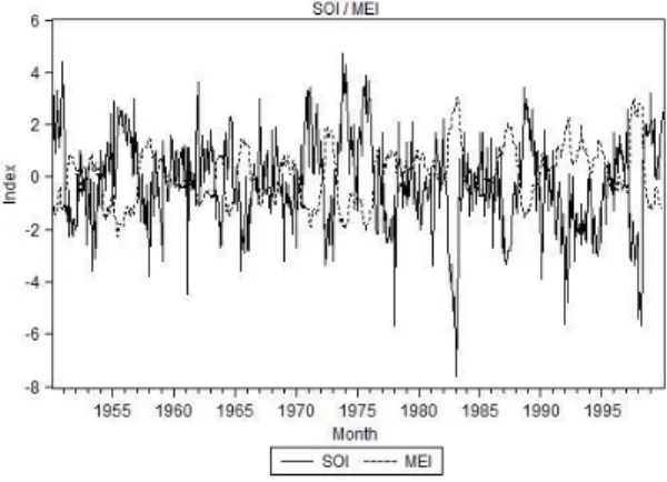
There are several indicators that provide information about the state of ENSO at a given time. One of them is the Southern Oscillation Index (SOI), which is calculated from the monthly fluctuations in the air pressure difference between Tahiti and Darwin. Sustained negative values of the SOI indicate El Niño episodes, while sustained positive values of the SOI indicate La Niña episodes. Another indicator of ENSO is the Multivariate ENSO Index (MEI). It is a monthly measure based on the six main observed variables over the tropical Pacific. MEI contains information of the sea level pressure, surface wind (East - West), surface wind (North - South), sea surface temperature, surface air temperature and total cloudiness of the sky. In this case, sustained negative values of the MEI indicate La Niña episodes, and sustained positive values of the MEI indicate El Niño episodes. In Figure 1, we can observe the SOI and MEI from 1990 to 2000. In this decade, it is possible to observe two strong episodes of El Niño. The first occurred from July-1993 to December-July-1993, and the second from April-1997 to March-1998.
Poveda et al. (2010) reviewed the hydro-climatic variability of the Colombian Andes associated with El Niño-Southern Oscillation (ENSO) using records of rainfall, river discharges, soil moisture and a vegetation index (NDVI). Their conclusions point to define ENSO as the main forcing mechanism of interannual climate variability. Given the indexes that were described previously (SOI and MEI), they quantify the anomalies in the sea surface
temperature in terms of their sign, timing and magnitude. These studies indicate that ENSO indexes become important and valuable tools to describe several hydro-climatological variables in the region.
Figure 1: SOI and MEI (1990-2000).
Over time, several models have been developed to describe the behavior of the phenomenon. This effort has resulted in the atmospheric general circulation models (ACGMs). ACGMs base their forecasts of sea level temperature on the behavior of the atmosphere. It develops global coupled ocean-atmosphere general circulation models (Meehl,1990). Given the implicit complexity to model the weather physically, this kind of approach becomes accessible only for national institutions that have the technology and equipment needed. Another alternative that has been used to describe the behavior of the phenomenon is related to statistical models. Thus, predictions are based on the behavior of climate variables during the last years. This approach aims to identify correlations in order to establish patterns in the behavior of the relevant variables. Most statistical models that have been developed for climatic variables are based on the Box-Jenkins methodology (BoxJenkins,1976). These models can represent the basic structure of the time series, but they fail to reproduce the nonstationary behavior that exists in climatic variables. A source of non stationarity is the existence of cyclic patterns that determine the
behavior of the weather. For example, El Niño-Southern Oscillation (ENSO) is a cyclical process composed of a warm phase (El Niño) and a cool phase (La Niña).
Given the existence of cyclical processes, several models have been developed to include the fact of various changing regimes over time. For example, Ubilava et al. (2013) adopted a smooth transition autoregressive modelling framework to explain the sea surface temperature in order to forecast ENSO; they argued the advantage of nonlinear models to represent dynamic processes such ENSO. In order to model the weather, the introduction of a variable that represents the weather type (regime) can be seen in Zucchini et al. (2009) where Hidden Markov Models (HMM) were proposed for modeling the space-time evolution of daily rainfall.
Furthermore, James Hamilton (1989) proposes econometric time series which are composed of a Hidden Markov Model (HMM) and autoregressive models. In MS-AR models, several autoregressive models are used to describe the time evolution of the series and the switching between these different models is controlled by a Hidden Markov chain which represents the possible regimes. MS-AR models were extended by Andrew Filardo (1994) who incorporated time-varying transition probabilities (TVTP) between regimes. Since its publication, several applications of the model have been implemented. Ailliot et al. (2012) propose a Markov-Switching Autoregressive model to describe the behavior of wind time series obtaining a good fit to the data. Souza et al. (2010) used a Hidden Markov Model (HMM) to predict future crude oil price movements. Their results indicate that the proposed model might be a useful decision support tool. Walid et al. (2011) proposed a Markov Switching model to investigate the exchange rates for four emerging countries over the period 1994-2009. Yuan (2011) presents an exchange rate forecasting model which combines the multi-state Markov Switching model with smoothing techniques. Guo et al. (2010) focus on detecting hot and cold IPO (Initial Public
Offering) cycles in the Chinese A-share market using a Markov regime switching model. The hot and cold periods and their turning points are detected clearly (A hot period is related to positive market conditions). Fallahi et al. (2014) used Markov Switching models to identify and analyze the cycles in the unemployment rate and four different types of criminal activities in the US. Finally, Liu et al. (2006) developed a Markov regime Switching model with two regimes representing expansion and contraction to catch the cyclical behavior of the semiconductor business.
The main objective of this paper is to propose an MS-AR, in order to evaluate the pattern changes of ENSO along the time. This model contributes to the prediction of hydro-climatic variables, with significant practical implications for agriculture, hydropower generation, fluvial transport, natural hazards and disasters, and human health. Section 2 describes the proposed model analysing its advantages and shortcomings. Section 3 presents the steps followed for the model implementation. Finally, several concluding remarks are given in the last section.
2. THE PROPOSED – MARKOV SWITCHING AUTOREGRESSIVE MODELS (MS-AR)
ENSO is a cyclical phenomenon in which it is possible to identify two regimes over time (La Niña and El Niño). The behavior patterns during each of the two phases are opposite and differentiable. On the other hand, the duration and the change between regimes is variable over time. Also, there is uncertainty about the length of episodes or phase transitions. This group of characteristics are properly evaluated by the Markov Switching Autoregressive Model (MSAR) proposed by Hamilton (1989) and improved by Filardo (1994). In this section we present the model, its application and relevant considerations for its implementation.
Certain variables undergo episodes in which the behavior of the series seem to change quite
dramatically according to a set of regimes. The Markov Switching Autoregressive Model proposes a very tractable approach to model changes in regime. In order to develop a model that allows a given variable to follow a different time series process over time (𝑦𝑡), consider a first-order autoregression in which the constant term 𝑐 and the autoregressive coefficient 𝞍 might be different for each regime 𝑠𝑡 proposed:
𝑦𝑡 = 𝑐𝑠𝑡+ 𝜙𝑠𝑡 𝑦𝑡−1+ 𝜖𝑡 (1)
where 𝜖𝑡 ∼ i.i.d N(0, 𝜎2). In order to model the
change in regime over the time we use a Discrete Time Markov Chain (DTMC). Then, we define 𝑠𝑡 as a random variable that can assume values according to a state-space {1,2, . . . , 𝑁}. Also, the probability that 𝑠𝑡+1equals some particular value 𝑗 depends on the past only through the most recent value 𝑠𝑡:
𝑃 {𝑠𝑡+1= 𝑗 ⎸𝑠𝑡 = 𝑖 , 𝑠𝑡−1= 𝑘 … }
= 𝑃 {𝑠𝑡+1= 𝑗 ⎸𝑠𝑡= 𝑖 } = 𝑝𝑖𝑗 (2)
The transition probability 𝑝𝑖𝑗 gives the
probability that state 𝑖 will be followed by state 𝑗 in a one-step transition. It is often convenient to collect the transition probabilities in an (𝑁⨯𝑁)
matrix 𝑃 known as the transition probability matrix.
In this way, a MS-AR process is a discrete-time process with two components {𝑆𝑡, 𝑌𝑡}, for our case, 𝑌𝑡 denotes the monthly index of SOI with values in (−∞, ∞) and 𝑆𝑡 ∈ {Niño (1), Niña
(2)} represents the regime at month 𝑡. A MS-AR process is characterized by the following two conditional independence assumptions:
- The conditional distribution of 𝑆𝑡 given the values of {𝑆𝑡′}t′<tand {𝑌𝑡′}t′<tonly depends on the value of 𝑆𝑡−1. In this manner, we assume that the weather type 𝑆𝑡 is a first order Discrete Time Markov Chain.
- The conditional distribution of 𝑌𝑡 given the values of {𝑆𝑡′}t′<t and {𝑌𝑡′}t′<t only depends on the value of 𝑆𝑡 and
𝑌𝑡−1,..., 𝑌𝑡−𝑝 . In this manner, we assume
that the value of SOI 𝑌𝑡 is an
autoregressive process of order 𝑝 whose coefficients evolve in time according to the regime 𝑆𝑡.
Hamilton (1989) assumes Fixed Transition Probabilities (FTP) for the DTMC. The assumption that the transition probabilities are time-invariant, implies that the expected durations of phases do not vary over time. Due to the variability of the ENSO, this assumption might be too strong. El Niño occurs irregularly, with a recurrence ranging from two to eight years with variation in intensity. Each episode lasts about six to fifteen months. On the other hand, La Niña occurs less frequently than El Niño, and an episode lasts from nine months to three years. Therefore, we implemented a Markov-Switching estimation procedure that incorporates time-varying transition probabilities (TVTP) into the Discrete Time Markov Chain (Filardo,1994). There are advantages to using a MS-AR (TVTP) against MS-AR(FTP):
- The TVTP model allows the transition probabilities to decrease or increase after a change of regime. In this way, TVTP models have the flexibility to identify systematic variations in the transition probabilities after turning points.
- The TVTP model captures more complex temporal persistence of the phases than an FTP model. Allowing the transition probabilities to change over time can represent long periods of an specific regime.
- The TVTP model permits time varying expected durations of the phases. It represents an strong advantage against FTP, in which the expected durations of phases are constant along the time.
The TVTP Markov-Switching model for the values of SOI, 𝑦𝑡 is presented below:
𝑦𝑡= 𝜇1+ Φ(𝐿)(𝑦𝑡−1− 𝜇𝑆𝑡−1) + 𝜖𝑡 𝑖𝑓 𝑠𝑡𝑎𝑡𝑒 1 (3)
𝑦𝑡= 𝜇2+ Φ(𝐿)(𝑦𝑡−1− 𝜇𝑆𝑡−1) + 𝜖𝑡 𝑖𝑓 𝑠𝑡𝑎𝑡𝑒 2 (4)
where Φ(𝐿) = 𝜙1+ 𝜙2𝐿 + ⋯ + 𝜙𝑟𝐿𝑟−1 is the
lag polynomial, 𝜇𝑆𝑡 is the state-dependent mean,
𝜖𝑡 ∼ i.i.d N(0, 𝜎2) and 𝑆𝑡 ∈ {Niño (1), Niña (2)}.
The variation from the FTP model presented above appears in the transition probabilities matrix.
𝑃 {𝑆𝑡+1= 𝑠𝑡+1 ⎸𝑆𝑡= 𝑠𝑡 , 𝑧𝑡}
= [1 − 𝑝𝑝11(𝑧𝑡) 1 − 𝑝11(𝑧𝑡)
22(𝑧𝑡) 𝑝22(𝑧𝑡) ] (5)
3. IMPLEMENTATION
This section presents the implementation of the ENSO indexes, along with the description of our proposed methodology. First, it is necessary to identify the order of the autoregressive model 𝑝 to capture the dynamic nature of the phenomenon. During this step, the autocorrelation function (ACF) and partial autocorrelation function (PACF) plots permit to identify the numbers of autoregressive terms that are needed, the estimation of the parameters including autoregressive coefficients and transition probabilities. Finally, we revise the model in order to determine whether the specified and estimated model is adequate.
During the MS-AR model specification, the number of regimes and the order 𝑝 of the autoregressive process were obtained. For our particular model, we defined two regimes trying to represent each phase of the ENSO. In this way, the state space of the DTMC is 𝑆𝑡 ∈ {Niño (1), Niña (2)}. A third state associated with the neutral phase was not specified because it can increase the complexity of the model without any additional advantage. Moreover, the results obtained support the proposal of having only two states. On the other hand, we proposed an autoregressive processes of order 𝑝 based on the
autocorrelation function (ACF). The ACF for lags one and two (months) is considerable and
significant; thus, the autoregressives process are going to follow this:
𝑦𝑡= 𝑐1+ 𝜙11𝑦𝑡−1+𝜙21𝑦𝑡−2+ 𝜖𝑡 𝑖𝑓 𝑠𝑡𝑎𝑡𝑒 1 (6)
𝑦𝑡= 𝑐2+ 𝜙12𝑦𝑡−1+𝜙22𝑦𝑡−2+ 𝜖𝑡 𝑖𝑓 𝑠𝑡𝑎𝑡𝑒 2 (7)
where 𝜙𝑖𝑗represents the autoregressive coefficient of order 𝑖 for regime 𝑗, 𝑐𝑗 is the constant of the
process for regime 𝑗 ∈ {Niño (1), Niña (2)} and 𝜖𝑡 ∼ i.i.d N(0, 𝜎2) is a white-noise process.
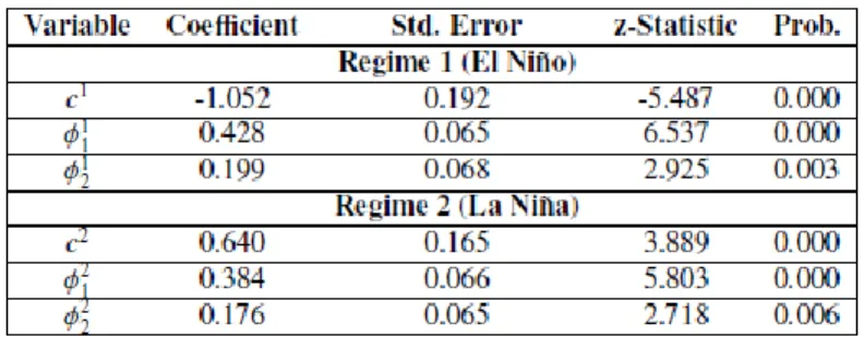
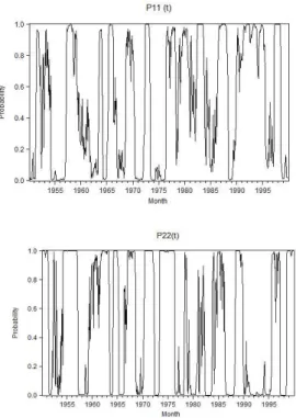
The data set presented in Figure 1 that was used to build the model has a monthly record since 1950 to 2000 and was downloaded from the National Climatic Data Center (NCDC) web site (National Climate Data Center, 2013). Given the model specification, the estimation of the autoregressive coefficients and the transition probabilities were developed in the computational software Eviews 8. The estimation method used by the software is maximum likelihood, whose output is shown in Table 1. As it can be observed in Table 1, each one of the estimated coefficients is statistically significant (𝑃𝑟𝑜𝑏. < 0.05). Consequently, the MS-AR(2) model is statistically significant to represent the data series of SOI. Furthermore, the estimation of the transition probabilities required in the model was also carried out. Note that the transition probabilities change over time (TVTP); the results are presented in Figure 2.
Figure 2: Time Varying Transition Probabilities
As it can be seen in Figure 2, the transition probabilities of remaining in the same state (𝑝11, 𝑝22) are approximated to one or zero for
various periods. Each of these periods represent an historical episode of El Niño or la Niña. Thus, during the months in which an episode of El Niño occurred, the probability of remaining in regime 1 (𝑝11) is close to one. On the other hand, during
these time intervals, the probability of remaining in regime 2 (𝑝22) is close to zero. For example,
one historical event of El Niño took place during 1993. For this year, we can clearly observe the related behavior in Figure 2. As it might be expected, the same pattern can be observed during historical episodes of La Niña. A clear example could be the episode of 1975.
In Figure 3, historical episodes of El Niño are shaded in orange. During these time intervals, it can be seen that the probability of being in state 1 (El Niño) is approximately one. Likewise, historical episodes of La Niña are shaded in blue. For these time periods, the probability of being in state 1 (La Niña) is close to zero. Also it can be
seen that during the periods in which there is no El Niño or la Niña events, the behavior of the probability of being in state 1 is unclear. Based on these probabilities, we preformed a validation process for the model. The duration of each of the episodes based on the model was identified and compared against the historical reports. The results obtained indicate that the model adequately captures the duration of episodes of both regimes.
From the transition probabilities, it is possible to infer the occurrence of El Niño and la Niña episodes. In this way, the MS-AR model allows to make inferences about when the episodes have occurred based on the observed behavior of the series. In Figure 3, the conditional probability of being in state 1 (El Niño) given the two previous observations of 𝑦𝑡 (𝑃[𝑆𝑡 = 1 ⎸ 𝑦𝑡, 𝑦𝑡−1 , 𝑦𝑡−2]) is plotted. As we only have
two states, the probability of being in state 2 (La Niña) is computed as the probability complement.
Figure 3: Conditional Probability of being in El Niño regime
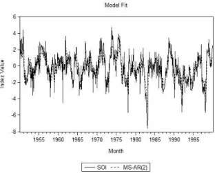
After the estimation of all the parameters of the MS-AR model, we verified its fitting to the data. It can be observed in Figure 4 that the proposed model captures the behavior of the index over time. It identifies the peaks and drastic changes in SOI along time. Likewise, it follows the trends observed during the historical episodes. When values remain positive or negative, the model reproduces the same pattern.
Figure 4: MS-AR(2) Fit
The final stage of the implementation consists of verifying the fit of the model by analyzing the residuals. The differences between the fitted model and the real series should follow a white-noise process. Thus, it was assessed with statistical tests that the expected value of the residuals is zero. On the other hand, to verify that the residuals are not correlated, the corresponding autocorrelation function (ACF) was developed, and as a result of this we concluded that the residuals are not correlated for any lag.
4. CONCLUSIONS
This paper investigates the use of MS-AR model to describe time series associated with ENSO. Our methodology is based on a two regime Markov Switching Autoregressive model that allows separate estimation between El Niño and La Niña episodes. The obtained results indicate that the model fits well to the time series. The proposed model is a very tractable approach to model time series with clear changes along the time. It is useful to describe variables in which is possible to identify various regimes fluctuating between them. This is the main advantage of the method against the Box-Jenkins methodology that has been widely used in this field. Box-Jenkins methodology leads to a good description of the time series, but it does not capture certain
non-linearities that occur due to the existence of changing regimes. Moreover, Box-Jenkins methodology does not allow to perform forecasts in long-term. In the study of climatic variables, one source of non-linearity in many meteorological time series is induced by the existence of weather cycles. Thus, the introduction of the cyclical phases of El Niño and La Niña allows to describe in a proper way the ENSO patterns.
The second advantage presented in the paper refers to the ability of the Markov Switching Model for defining and measuring cycles in a time series. With the model it is possible to draw probabilistic inference about whether and when they may occur based on the observed behavior of the series. This fact allows to discover regimes that are not directly observable and that could be used as explanatory factors of the variables in evaluation. Moreover, the interpretation of the model leads to open structure which allows more physical models. Models which consider the physical behavior of the phenomena to statistically explain the variables in analysis. On the other hand, the estimation of parameters by the method of maximum likelihood provides the foundation for forecasting future values of the series.
As the main concluding remark, the Markov Switching Autoregressive Model is a methodology that can represent time series with changing regimes over time. In our particular application, the model explain the cyclical variability of the phenomenon properly.
5. REFERENCES
Box, G.E.P, J. G., 1976. Time Series Analysis, Forecasting and control. Holden-Day.
Center, N. C. D., August 2013. Climate information. URL http://www.ncdc.noaa.gov/climate-information Fallahi, F., R. G., 2014. Link between unemployment
and crime in the us: A markov-switching approach. Social Science Research, 33–45. Filardo, A., 1994. Business-cycle phases and their
transitional dynamics. Journal of Business and economic statistics, 299–308.
Guo, H., B. R. S. R., 2010. Detecting hot and cold cycles using a markov regime switching model - evidence from the chinese a-share ipo market. International Review of Economics and
Finance, 196–210.
Hamilton, J., 1989. A new approach to the economic analysis of nonstationary time series and the business cycle. Econometrica, 357–384. Liu, W., C. Y., 2006. A markov regime-switching
model for the semiconductor industry cycles. Economic Modelling, 569–578.
Meehl, G., 1990. Development of global coupled ocean-atmosphere general circulation models. Climate Dynamics, 19–33.
Meehl, G., 2000. Trends in extreme weather and climate events: Issues related to modeling extremes in projections of future climate
change. Bulletin of the American
Meteorological Society, 427–436.
Oceanic, N., Administration, A., April 2010. Enso. URL http://www.oar.noaa.gov/k12/html/elnino2.html Poveda, G., A. D. R. O., 2010. Hydro-climatic
variability over the andes of colombia associated with enso: a review of climatic processes and their impact on one of the earth’s most important biodiversity hotspots. Climate Dynamics, 19–33.
Souza e Silva, E.G., L. L. S. e. S. E., 2010. Forecasting oil price trends using wavelets and hidden markov models. Energy Economics, 1507– 1519.
Walid, C., C. A. M. O. F. J., 2011. Stock market volatility and exhange rates in emerging countires: A markov-state switching approach. Emerging Market Review, 272–292.
Yuan, C., 2011. Forecasting exchange rates: The multi-state markov-switching model with smoothing. International Review of Economics and Finance, 342–362.
Zucchini, W. McDonald, I., 2009. Hidden Markov Models for Time Series: An introduction. Chapman Hall/CRC.


