An individual-based evolving predator-prey ecosystem simulation using a fuzzy cognitive map as the behavior model

To link to this article: DOI: 10.1162/artl.2009.Gras.012

URL

:

http://dx.doi.org/10.1162/artl.2009.Gras.012

This is an author-deposited version published in: http://oatao.univ-toulouse.fr/

Eprints ID: 7999

To cite this version:

Gras, Robin and Devaurs, Didier and Wozniak, Adrianna and Aspinall, Adam

An individual-based evolving predator-prey ecosystem simulation using a fuzzy

cognitive map as the behavior model. (2009) Artificial Life, vol. 15 (n° 4). pp.

423-463. ISSN 1064-5462

O

pen

A

rchive

T

oulouse

A

rchive

O

uverte (

OATAO

)

OATAO is an open access repository that collects the work of Toulouse researchers

and makes it freely available over the web where possible.

Any correspondence concerning this service should be sent to the repository

An individual-based evolving predator-prey ecosystem simulation

using Fuzzy Cognitive Map as behavior model

Gras R.*, Devaurs D.*, Wozniak A.*, Aspinall A.* * University of Windsor, School of Computer Science

Correspondence to: R. Gras, University of Windsor, 401 Sunset Avenue, N9B 3P4 Windsor, Ontario, Canada. rgras@uwindsor.ca, +1 519 253 3000 ext. 2994

Abstract

This paper presents an individual-based predator-prey model with, for the first time, each agent behavior being modeled by a Fuzzy Cognitive Map (FCM), allowing the evolution of the agent behavior through the epochs of the simulation. The FCM enables the agent to evaluate its environment (e.g., distance to predator/prey, distance to potential breeding partner, distance to food, energy level), its internal state (e.g., fear, hunger, curiosity) with memory and choosing several possible actions such as evasion, eating or breeding. The FCM of each individual is unique and is the outcome of the evolution process throughout the simulation. The notion of species is also implemented in a way that species emerge from the evolving population of agents. To our knowledge, our system is the only one that allows modeling the links between behavior patterns and speciation. The simulation produces a lot of data including: number of individuals, level of energy by individual, choice of action, age of the individuals, average FCM associated to each species, number of species. This study investigates patterns of macroevolutionary processes such as the emergence of species in a simulated ecosystem and proposes a general framework for the study of specific ecological problems such as invasive species and species diversity patterns. We present promising results showing coherent behaviors of the whole simulation with the emergence of strong correlation patterns also observed in existing ecosystems.

Keywords

Evolving ecosystem, predator-prey model, individual-based model, Fuzzy Cognitive Map, speciation

1 Introduction

Individual-based modeling is a bottom-up approach to simulating ecosystems that allows for the consideration of the traits and behavior of individual organisms. Whereas classical approaches to modeling ecology often ignore individual behavior and instead consider an entire ecosystem as a whole, individual-based models aim to "treat individuals as unique and discrete entities" [10]. By modeling individuals with varying ages, social ranks, and adaptability, for example, the properties of the system that the individuals represent can begin to emerge. This has a distinct advantage over classical approaches, namely that the assumptions made regarding individual behavior (such as the desire for fitness and shelter) provide for a more detailed simulation than using a state-variable model that may begin by calculating birth and death rates.

It has been suggested that because models are not well categorized, it is difficult to isolate any one model as being a specific type, such as individual-based [38]. Critics of this approach suggest that individual-based models are merely a tool for simulating very specific environments. However, advocates who favor the use of individual-based models are driven by paradigmatic motivation [10] where such models may be used to formulate general theories of ecology. The generality of individual-based modeling is an important area of consideration. As beneficial as a specific model may be, it is often more worthwhile to formulate general theories. The authors of Individual-based Modeling and Ecology reserve several sections to discuss the generality of individual-based models [11]. They describe the difficulty of creating generic ecological models by comparing ecology to physics. "Individuals [of ecology] are not atoms but living organisms" and because "individual organisms have properties an atom does not have", such as the variation between them and their adaptive behavior, aiming for generality in ecological models is much more difficult. Despite this, there continues to be a rise in the use of individual-based models [16].

While the use of individual behavior has been included in many models during recent decades [15], the individual-based modeling approach is exponentially increasing as the cost to purchase and operate a machine capable of running time consuming simulations reduces. The contributions of individual-based models are discussed in [4] which examines, among others, how forest ecology [32], a fish-recruitment model [29], and models depicting spatial heterogeneity [18] have all benefited from this approach. Few attempts have been made to model a complete ecosystem. A pioneer in this domain is J. Holland with his platform Echo [12, 13] which includes an evolutionary mechanism. However, the organisms in Holland’s simulation are very simple and do not involve any behavioral model. A predator-prey model has also been proposed by Ward et al. [39], with more complex agent models. Nevertheless, the agent model is dedicated to represent schooling behaviors and the evolution is an offline mechanism using a genetic algorithm. More recently, Ronkko [30] has proposed a high scale simulation based on a particle system approach. There is, however, no evolution mechanism in this artificial ecosystem.

As the agent behavioral model is crucial to creating complex interacting agent, we have chosen a sophisticated but efficient model called Fuzzy Cognitive Map (FCM) [17]

to model the agents’ behavior. In our simulation, FCM is not only the base for describing and computing the agent behaviors, but also the platform for modeling the evolutionary mechanism and the speciation events. Additionally, we have implemented a speciation mechanism based on gene pool and, to our knowledge, for the first time in such simulation, linked behavioral patterns to speciation. To date, there is also no large scale individual-based ecosystem simulation that integrates a complex behavioral model for the agents, an evolutionary mechanism and a speciation mechanism. In particular, there is no use of FCM or equivalent model in such a large scale simulation and in the context of evolution. Our study includes important ecological and evolutionary concepts at a computationally acceptable cost. As we include in the same timescale of the simulation speciation events and individual behaviors, we have chosen to only represent tendency of behavior for our individuals. Therefore, a time step in the simulation represent a relatively long time period. The individuals perform multiple actions during this period but with a specific tendency corresponding to the action represented in our simulation (section 3.3). We show that such complex adaptive systems lead to a generic ecosystem with behaviors similar to those found in existing ecosystems. These are the key components needed in order to show that this kind of approach can be used to understand existing ecosystems and make some interesting and valid predictions.

The rest of the article is organized as follows: In section 2, we present and define the FCM model. In section 3, we describe the agents, the speciation concepts, the evolutionary mechanism and all the other components of our simulation. In section 4, we show the results we obtained for one run of the simulation and discuss about the pertinence of these results considering existing ecosystem behaviors. Finally in section 5 we conclude about this work and propose several possible extensions and dedicated applications to enhance our method.

2 Fuzzy Cognitive Maps

The Fuzzy Cognitive Maps rely on a concept derived from cognitive maps that was originally introduced by psychologists to model complex behaviors [36]. Recently, these FCMs have been extended in several steps: formalization as an oriented graph [1], association with fuzzy logic (Fuzzy Cognitive Map) [17], dynamic integration of external information [34] and learning [35]. FCMs aim to represent the causal relationship between concepts and to analyze inference patterns (the final state of the system after convergence). They are able to handle temporal information and fuzzy activation levels for each concept. They have been used in a wide variety of fields involving economic system modeling [33], machine learning [9], freeway modeling [37], autonomous agent modeling [34], etc. FCMs have also been used to represent complex biological systems such as ecosystems [26] and regulatory networks [41, 5]. FCMs have been used to model individual agent behaviors [34, 35] but only for few none evolving individuals. This last application led to very promising results that demonstrate the ability to represent complex internal concepts as emotions and desires, and to build agents that are able to perceive, make decision and act. Nevertheless, to our knowledge, a FCM has never been used in a large scale individual-based modeling of an ecosystem and has never been used in an evolutionary context.

We used mostly the definition of the FCM coming from [34]. FCMs are graphs which contain a set of nodes C, each node Ci being a concept, and a set of edges I, each

edge Iij representing the influence from a concept Ci to a concept Cj. A positive value of

Iij corresponds to an excitation of the concept Cj from the concept Ci whereas a negative

value corresponds to an inhibition (a value of 0 meaning that there is no influence of Ci

on Cj). An activation level ai is also associated to each concept. The FCM allows the

computation of the value of the concepts of an agent based on its perception and on the current activation level of its concepts. This computation is called the dynamic of the map and is a normalized matrix product (see section 2.1)

The FCM is used to model the agent behaviors (structure of the graph) and to compute the next action of the agent (dynamic of the map). A map contains three kinds of concepts: sensitive, internal and motor. The activation level of a sensitive concept is computed by a fuzzification of the information coming from the environment. The activation level of the motor concept is used to determine what the next action of the agent will be and a defuzzification of its value can be used to determine the amplitude of the action. Finally, the internal concepts’ activation level corresponds to the level of intensity of the internal states of the agent and affects the computation of the dynamic of the map.

2.1 A formal definition of FCM

A FCM F is a quadruplet (C, L, A, R) where: • C = {C1, …, Cn} is the set of n concepts

• L is a matrix n x n with Lij ∈ ℜ. Lij is the influence of concept Ci on concept Cj. If Lij

= 0, there is no edge between Ci and Cj.

• ),...} 1 ( ), 0 ( { ] 1 , 0 [ i i i a a C C A → → = ℵ

is a function that associates the series of all its successive activation levels to each concept Ci such as for t ∈ℵ, ai(t) ∈ [0,1] is its activation

level at time t.

• R is a recursive relation between ai(t+1) and ai(t) with 1≤i≤n which describes the

dynamic of the map F.

) ) ( ), ( ( ) 1 ( , , 1 ; 0 ) ( , 1 1 0 0

∑

where g : ℜ2_{→ℜ is a function such as: min(x,y) or max(x,y) or αx + βy, and where}

σ : ℜ→ [0,1] is a normalization function with two possible modes:

(a) continuous mode, where σ is the sigmoid function σ(δ,a0,k) centered in (a0

,(1-δ)/2) with a slope of k.(1+ δ)/2 in a0 and with limits in ±∞ respectively of 1 and 0:

) ( ) , , ( 0 0

1

1

]

1

,

0

[

:

e

a

+

→

→

ℜ

σ

2 2 1 1 2 1 1 1 0 : s a if s a s if s s s a s a if a > ≤ ≤ − − < → σ 2.2 A simple example

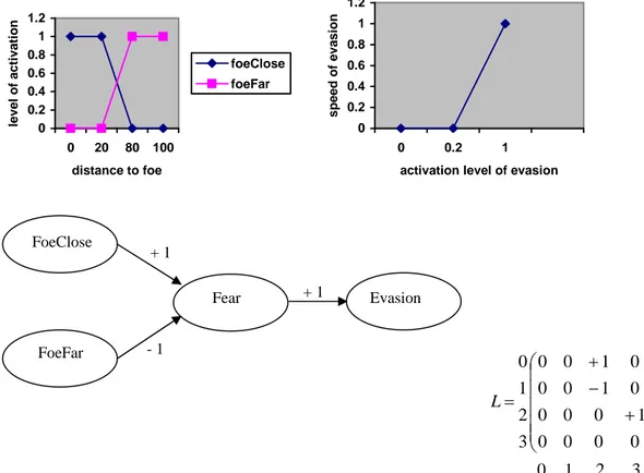
A very simple map can be defined to model an agent perceiving and reacting to its distance to a foe. The closer the foe, the more frightened the agent. Depending on this distance and then on the fright level the agent will decide whether or not it will evade. The more frightened the agent, the faster the evasion. An FCM corresponding to this example is given in figure 1. In this example there are two sensitive concepts: foeClose and foeFar, one internal: fear and one motor: evasion. There are also three influence edges: closeness to a foe excites fear, distance to a foe inhibits fear and fear causes evasion. Activations of the concepts foeClose and foeFar are computed by fuzzyfication of the real value of the distance to the foe, and the defuzzyfication of the activation of

evasion tells us about the speed of the evasion.

0 0.2 0.4 0.6 0.8 1 1.2 0 20 80 100 distance to foe level o f acti vati o n foeClose foeFar 0 0.2 0.4 0.6 0.8 1 1.2 0 0.2 1

activation level of evasion

speed o f eva si o n 3 2 1 0 0 0 0 0 1 0 0 0 0 1 0 0 0 1 0 0 3 2 1 0 ⎟⎟ ⎟ ⎟ ⎟ ⎠ ⎞ ⎜⎜ ⎜ ⎜ ⎜ ⎝ ⎛ + − + = L

Figure 1. A simple fuzzy cognitive map for detection of foe and decision to evade with its corresponding matrix L and 0 for “Foe close”, 1 for “Foe far”, 2 for “Fright” and 3 for “Evasion” and the fuzzyfication and defuzzyfication functions.

Evasion Fear FoeClose FoeFar + 1 + 1 - 1

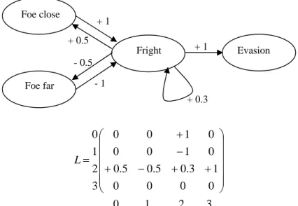
With the FCM model it is possible to distinguish the perception from the sensation: the sensation is the real value coming from the environment and the perception is the sensation modified by the internal states. For example, it is possible to add three edges to the previous map (figure 2): one auto-excitatory edge from the concept fear to itself, an excitatory edge from fear to foeClose and one inhibitory edge from fear to foeFar. A given real distance to the foe seems higher or lower to the agent depending on the activation level of fear. Also the fact that the agent is frightened at time t influences the level of fright of the agent at time t + 1. This kind of mechanisms gives the possibility to model a degree of paranoia and a degree of stress for the agent. It also allows to memorize information from previous time steps: fear maintains fear. If the dynamic of the map is computed several times using the same sensation value (several applications of R updating each time the values of the concepts) it allows the sensitive information to go through each level of the map, even if there are loops, and influences the motor concepts before any action is undertaken. As a decision making model that can be understood as: take time to think before acting. It is therefore possible to build very complex dynamic systems involving feedback and memory using FCM, which is what is needed to model complex behaviors and abilities to learn from evolution.

3 2 1 0 0 0 0 0 1 3 . 0 5 . 0 5 . 0 0 1 0 0 0 1 0 0 3 2 1 0 ⎟⎟ ⎟ ⎟ ⎟ ⎠ ⎞ ⎜⎜ ⎜ ⎜ ⎜ ⎝ ⎛ + + − + − + = L

Figure 2. A simple fuzzy cognitive map for detection of foe and decision to evade with its corresponding matrix L and 0 for “Foe close”, 1 for “Foe far”, 2 for “Fright” and 3 for “Evasion”.

3 An evolving ecosystem

We have chosen an individual-based approach for our simulation of an evolving ecosystem. We aimed to develop a generic platform able to simulate complex ecosystems with “intelligent” agents interacting and evolving in a large and dynamic environment. An important property that we wanted to integrate was the fact that the agents have to develop efficient behaviors to be able to survive in this environment. We have therefore chosen a predator-prey model in which behaviors of preys and predators have to evolve

Evasion Fright Foe close Foe far + 1 + 1 - 1 + 0.3 + 0.5 - 0.5

simultaneously to give them abilities to survive. Our ecosystem is composed of individuals belonging to two trophic levels: prey and predator. We also handle two resources: grass and meat which are respectively the food for the preys and the predators (see section 3.3). This concept could be easily applied to a more complex food chain by adding more resources and creating a higher hierarchy of predator/prey. Each agent possesses its own genome (the matrix L of its FCM, see section 3.1), can interbreed with other genetically similar individuals and produce offspring with a modified combination of the genomes of its parents (see section 3.5). We also represent species (see section 3.2). New species can emerge from the evolution of individuals and get extinct if all their members die.

3.1 Agents

Each agent has several properties that determine its physical capabilities and its behaviors. The Behaviors are determined by the interaction between the FCM and the environment. Each agent possesses its own FCM that represents its genome. This FCM contains sensitive concepts: (1) foeClose (prey only), (2) foeFar (prey only), (3)

preyClose (predator only), (4) preyFar (predator only), (5) foodClose, (6) foodFar, (7) mateClose, (8) mateFar, (9) energyLow, (10) energyHigh, (11) quantityOfLocalFoodHigh, (12) quantityOfLocalFoodLow, (13) quantityOfLocalMateHigh, (14) quantityOfLocalMateLow; internal concepts: (15) hunting (predator only), (16) fear, (17) hunger, (18) sexualNeeds, (19) curiosity, (20) sedentarity, (21) satisfaction, (22) annoyance; and motors concepts: (23) evasion (prey

only) , (24) searchForPreys (predator only), (25) searchForFood, (26) socialization, (27)

exploration, (28) resting, (29) eating, (30) breeding. It also contains links and weights

representing the mutual influences of these concepts. Concepts (1) to (8) are computed by the fuzzyfication (using ternary mode (b) from section 2.1) of the distance of the closest corresponding feature (foe, prey, food and mate). Concepts (11) and (12) are computed by the fuzzyfication (using ternary mode (b) from section 2.1) of the number of food units currently available in the cell of the agent. Concepts (13) and (14) are computed by the fuzzyfication (using ternary mode (b) from section 2.1) of the number of possible mates currently present in the cell of the agent. The FCM of an agent is transmitted to its offspring after being combined with the one of the other parent and after the possible addition of some mutations. The behavior model of each agent is therefore unique1. Links between concepts can appear or disappear during this process so the structure and complexity of the map can also change during the evolutionary process.

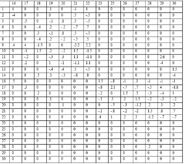
The values of the FCM used to initialize all first preys and predators are given in tables 1 and 2. It is important to notice that such a behavioral model allows the representation of very complex phenomena. For example, looking at table 1, it appears that the concept of evasion is excited by the concepts of fear and annoyance and inhibited by the concepts of hunger, sexualNeeds, curiosity and satisfaction. These concepts in turn are excited or inhibited by all the sensitive concepts. That means that the activation level of the motor concept of evasion depends on a complex and non-linear combination of all the sensitive concepts and of 6 internal concepts. This is true for all the motor concepts. Another important thing to notice is that the activation levels of all the concepts of an

1 _{In fact, the uniqueness is not guaranteed but the probability that two identical FCM appears during the}

agent are never reset during its life. As the previous time step activation level of a concept is involved in the computation of its next activation level, it means that all the previous states of an agent during its life participate in the computation of its current states. It means therefore that an agent has a memory of its own past that will influence its future states. As the action undertaken by an agent at a given time step depends on the current activation level of all its motor concepts, the global behavior of an agent dynamically depends on a complex combination of all the information it currently receives from its environment, all its current internal states and all the past states it went through during its life.

Table 2. Initial matrix L for predators

The physical capabilities are:

• Maximum and current level of energy. At each time step, each agent spends energy depending on its action (breeding, eating, running…) and on the complexity of its behavior model (number of nodes and edges in its FCM). The more complex its model is, the more energy the agent spends at each time step. The maximum level of energy (maxEnergyPrey and maxEnergyPredator) is associated with the type of agent (predator or prey).

• Maximum and current age. The maximum age (maxAgePrey and

maxAgePredator) of an individual is determined randomly at birth from a

distribution centered at a value associated with the type of agent. At each time step the age of each agent is incremented by one. When the current age of an agent is equal to its maximum age it dies.

• Minimum age for interbreeding. The minimum age at which an individual can begin to interbreed is associated with the type of agent (ageInterbreedPrey and

ageInterbreedPredator).

• Maximum and current speed. The current speed of an agent is calculated when it undergoes a moving action. The speed value corresponds to the defuzzification of the activation level of the corresponding motor concept. The maximum speed is associated with the type of agent (maxSpeedPrey and maxSpeedPredator).

• Vision distance. This parameter determines how far (in number of cells) an agent can perceive things (food, foe…). The vision distance is associated with the type of agent (distanceVisionPrey and distanceVisionPredator). At most each individual can view and memorize the 5 closest individuals and resources of each type within its vision range.

• The energy transmitted to offspring. It determines the minimum percentage of energy that is transmitted to the (unique) offspring from its parents (see section 3.6). The maximum percentage is birthEnergyPreyMax for the preys and

birthEnergyPredatorMax for the predators. The level of energy of the offspring is

uniformly selected between these minimum and maximum values. Each parent looses half of this value. The amount of energy transmitted from the parents to their offspring is also submitted to evolution. The energy value for the offspring is the value (possibly mutated) of one of the two parents. The energy transmitted to the offspring is initially associated with the type of agent (birthEnergyPrey and

birthEnergyPredator)2.

3.2 Species

To the best of our knowledge, there were two models embodying mechanism of speciation: species were migrating and getting extinct but did not originate and the number of species was a predefined parameter. We have built a model implementing speciation mechanism that is related to the genotypic cluster definition proposed by Mallet [16]. The speciation mechanism we implemented accounts also for the gradualism and fuzziness of the speciation process. Traditionally, good species are populations that do not exchange genes with other populations so that there is no blurring of the species border: “species level is reached when the process of speciation has become irreversible,

even if some of the (component) isolating mechanisms have not yet reached perfection

[23]3. Yet, our model accounts for the fact that isolating barriers operating between populations and delimiting species boundaries undergo evolution, so that their appearance in itself is a part of speciation [21]. What is more, these boundaries are not permanent over time. For example, in the case of young related species we cannot exclude the possibility that even species considered as good will backcross, i.e. fuse back into one via hybridization. Indeed, recent studies have shown that hybridization is frequent (Cichlids in African lakes, common in plants). Our model accounts for the fact that speciation is not always a sharp and clear-cut process and that there are numerous groups showing substantial reproductive isolation but also exchange genes with sympatric relatives to some degree [2]. Thus, with these assumptions we can ask ourselves a few questions, such as A) how exactly intergradation takes place, implicit in the gradual nature of evolution, which presupposes the presence of intermediating forms, and B) what about the origin of speciation in sympatry, driven by behaviour (such as mating preferences).

2 _{These two parameters are used to initialise the populations of preys and predators at the first time step. As}

these parameters are subjected to evolution, they are specific to each agent been born during the simulation.

3 _{Similarly according to some of those who plead for sympatric speciation, the gene flow should approach}

A) Indeed, one of the problems the simulation allows us to tackle with, is the problem of speciation, i.e. the origin of discrete groups of organisms [3, 7] or, in other words, the origin of organic diversity and the level at which the evolutionary process of differentiation is concerned. Yet, Darwinian evolution, synonymous to speciation, is considered a gradual process. Thus, a number of biologists have argued that gradual nature of the process of evolution implies gradual character of speciation [3, 22, 25]. We propose a model that accounts for speciation as a quasi-continuous process that yields intermediate stages.

B) Indeed, the innovation of our ecosystem simulation lies in the fact that it encompasses a complex behavioural model for the agents altogether with a speciation mechanism. We can then also examine the potential role of non-genetically driven individual variation, such as behaviour, or learning, in generating local selective pressure. This is crucial to determine whether reproductive isolation must be genetic or can have ontogenetic, and particularly behavioural basis, e.g. in sympatric speciation.

In our simulation a species is a set of individuals associated with the average of the genetic characteristics of its members. The average map is computed on the basis of the FCM matrixes of all individuals that are members of a species. It is considered that an individual belongs to a species if the difference between its matrix and the average matrix of the species is below a speciation threshold; the speciation threshold is the same for all species. Interbreeding can take place if the distance between individual matrixes is below the reproductive threshold. When a newborn appears, the distance between its matrix and the average matrixes of all existing species is computed. If the distance with respect to the closest average (i.e. the more similar species) is greater than the speciation threshold, then the individual forms a new species S. If in subsequent time-steps matrixes of some individuals turn out to be closer to S rather than to the average of their original species, the membership of these individuals will be switched to that new species.

More formally, we define a species as a set of individuals S and a centre C(S) that represents the average genome of its members. We then define a metric D, such that D(x,y) is the distance between the genomes of two individuals x and y:

∑

with Lijx (resp. Lijy) the edge between concepts i and j in the matrix L of x (resp. y). The

center C(S) is a matrix Lc(S) such as:

S L S L n j n i j i x S x ij c ij

∑

Then, it is also possible to compute the distance between an individual x and a species S:

∑

Considering the current set ∑ of existing species, an individual x is a member of a species S if: )) ' , ( ( min ) , ( ' D x S S x D S∈Σ =

Using the metric D and a speciation threshold T, a speciation event appears when a new offspring x is born such that: ∀S∈∑ D(x,S) > 2*T. Considering two individuals possibly

from two different species), we define the probability P(x,y) that these individuals can interbreed by: otherwise T y x D if y x D f y x P 0 ) , ( )) , ( ( ) , ( = ≤

with f: [0,T]→[0,1] a decreasing function of D(x,y).

3.3 The world

Our simulation takes place in a toric virtual world composed of 1000 cells in both dimensions. Each cell can contain resources (grass and meat) and an unlimited number of individuals of both kinds. Because we want to focus on evolution of populations, we have chosen to make a coarse grain simulation. Even if every individual is simulated independently with a complex behavior, the world is not considered in high details. Therefore, a cell represents a large space that can contain an unlimited number of individuals. There is however a limit in the amount of resource available in each cell. This allows a competition for resource between individuals to occur.

We have also chosen an almost (see below) synchronous mode with discrete time. A time step corresponds to: the computation of all the agents’ sensitive concepts, the computation of several dynamics of the map for each agent, the execution of one action by agents and the update of the parameters of the world. A time step also represents a relatively long time period. So, an action undertaken by an agent can in fact be viewed as a tendency. The agent performs a lot of small actions during a time step but the whole behavior is directed toward the realization of the given action. As a consequence, the total number of actions performed by each agent during its life is relatively small (a few dozens). This allows us to obtain a high level of population renewal which is an important criterion for studying an evolutionary process.

The maximum numbers of unit of each resource (maxGrass and maxMeat) by cell is a parameter of the simulation. At the initialization time there is no meat in the world and the number of grass units is randomly determined for each cell. For each cell, there is a probability, probaGrass, that the initial number of units is strictly greater than 0. In this case, the initial number is generated uniformly between 1 and maxGrass. Each unit provides a fixed amount of energy to the agent that eats it. The preys can only eat the grass and the predators have two modes of predation: hunting and scavenging. When a predator hunting action succeeds, new meat units are added in the corresponding cell. When a predator eating action succeeds (which can be viewed as a scavenging action), one unit of meat is removed in the corresponding cell. The amount of energy is

energyGrass for one grass unit when eaten by a prey and is energyMeat for one meat unit

eaten by a predator. The number of grass units grows at each time step (see section 3.4) and when a prey dies in a cell the number of meat units in this cell increases by 2. The number of grass units in a cell decreases by 1 when a prey eats and the number of meat decreases by 1 also when a predator eats. The number of meat units in a cell also decreases at each time step even if no meat has been eaten in this cell.

The initial position of the individuals is generated non-uniformly to form clusters of individuals. The idea is to model a realistic initial world state by having the individuals grouped in clusters. The parameter sizeClusterPrey (resp. sizeClusterPredator) sets how many preys (resp. predators) are members of each initial cluster. For the first member of the cluster, its position is uniformly generated in the whole world. Then, for all other

members of the cluster, their positions are uniformly generated among all cells that are in a sizeCluster-radius from the position of the first member. The initial number of preys (resp. predators) is determined by the simulation parameter initNbPrey (resp.

initNbPredator) which is a multiple of sizeCluster. At the first time step all preys (resp.

the predators) are members of the same species with a center corresponding to the initial FCM of preys (resp. predators) since all the individuals of the same type initially have the same FCM.

The preys and the predators are stored in two different lists in an age ascending order. We use this order to determine who acts before whom. For example, if in a given cell there is only one food unit and two agents that have chosen the action of eating, the youngest will act first and so it will be the only one that can eat (in this cell) at this time step. The action of the other one fails and it does nothing at this time step (except losing some energy). So even if every agent looks at its environment simultaneously, then makes a decision of action simultaneously, the simulation is not completely synchronic because there is an ordering of the actions based on the age of the agents. With this system the younger ones are advantaged compared to the older ones. It is a way to simulate the fact that the young can act faster than the old.

3.4 Update

At each time step we need to update the value of the state of all the parameters of our model. Here is the overview of the successive phases of the update process:

For every prey: Perception of the environment (1) For every prey: Computation of all concepts (2)

For every prey: Application of their action and update of the energy level (3) Updating the list of prey (4)

For every predator: Perception of the environment (1) For every predator: Computation of all concepts (2)

For every predator: Application of their action and update of the energy level (3) Updating the list of predators (4)

Updating the list of preys (5) Updating the prey species (6) Updating the predator species (6) For every cell in the world {

Updating the grass level (7) Updating the meat level (8) }

Updating of the age of the agents (9)

The steps (1) to (9) are detailed here (for the predator, steps (1) to (4) and (6) are similar to those of preys):

(1) For every prey, computation of the five closest foes; cells with food units and mates within the vision range of the prey; its current level of energy; the quantity of grass units in its cell; the number of possible mates in its cell are performed. The possible mates of a prey that is a member of a species S are the preys that are

members of a species S’ in which D(S,S’) < 2*T. With this mechanism we model the fact that an individual can evaluate its similarity with other individuals and then estimate if it can interbreed. This estimation is not precise because only the distance between their corresponding species is taken into account and with a threshold twice higher than the threshold for interbreeding. So individuals can try to interbreed even if mating will fails.

(2) For every prey, computation of: the value of its sensitive concepts by fuzzyfication of the previous values; three dynamics of the map by applying the recursive formula R given in section 2.1 three consecutive times. Function g is x + y. Function σ is the continuous mode (a) for the internal and motor concepts and the ternary mode (b) for computing the initial value of the sensitive concepts. (3) For every prey, in the age ascending order, application of the action

corresponding to the motor concept that has the highest activation level4 and computation of the corresponding speed of the prey. Then computation of its new energy level by applying the formula:

4 . 1 10 speed nbedges nbconcepts energy energy= − − −

with nbconcepts the sum of the number of sensitive, internal and the motors concepts, nbedges the number of edges in the prey FCM that have a value different from 0 and speed the distance traveled by the prey during this time step. (4) For every prey, removing it from the list and adding two meat units in its cell if its

energy is lower than or equal to 0 or if its age is greater than its maximum age. Adding all new prey’s offspring to the beginning of the list of preys.

(5) Removing from the list every prey that has been killed by the predators.

(6) Removing every member of the current prey species (the species are reset before reallocating the preys to their closest species). Then, for all prey p, in the age ascending order, applying the algorithm:

dmin = 0 Smin = ∅

For all species S in ∑ d = D(p,S) if d < dmin dmin = d Smin = S If (dmin < 2*T) S = S ∪ p Else

Create a new empty species S’ S’ = S’∪p

∑ = ∑∪S’

4 _{If the highest motor concept is breeding then it is also required that the age of the prey (resp. predator) is}

greater than ageInterbreedPrey (resp. ageInterbreedPredator) otherwise it is the action corresponding to the second highest motor concept that is chosen.

Then, removing every prey species that does not have anymore members, for every prey species S computing its new center C(S) and for every prey species S computing its distance D(S,S’) with all other species.

(7) For every cell of the world: if its number of grass units is greater than zero adding

growGrass units of grass else if one of its 8 adjacent cells has a level of grass

greater than zero adding growGrass units of grass with a probability of

probaGrowGrass. With this mechanism if the agents eat all the grass in one cell

the grass cannot grow anymore unless there is still grass in an adjacent cell. That prevents agents from staying in one place waiting for the grass to grow and models the problem of overexploitation of resource. That also models the mechanism of diffusion of resources through the world changing and renewing the interest of regions of the world. After this process if the number of grass units in the cell is greater than maxGrass, it is set to maxGrass.

(8) For every cell of the world: if its number of meat units is greater than zero subtracting decreaseMeat meat units. With this mechanism we model the fact that meat is perishable.

(9) Incrementation of the age of all agents. The possible actions for the agents are:

1) Evasion (for preys only). The evasion direction is the direction opposite to the direction of the closest foe within the vision range of the prey compared to the current position of the prey. If no predator is within the vision range of the prey the direction is chosen randomly. Then the new position of the prey is computed using the speed of the prey (see below) and the direction. The current activation level of fear is divided by two.

2) Search for food. The direction toward the closest food (grass or meat) within the vision range is computed. If the speed of the agent is high enough to reach the food, the agent is placed on the cell containing this food otherwise the agent moves at its speed towards this food.

3) Socialization. The direction toward the closest possible mate within the vision range is computed. If the speed of the agent is high enough to reach the mate, the agent is placed on the cell containing this mate and the current activation level of

sexualNeeds is divided by three otherwise the agent moves at its speed towards

this mate. If no possible mate is within the vision range of the agent the direction is chosen randomly.

4) Exploration. The direction is computed randomly. The agent moves at its speed in this direction. The activation level of curiosity is divided by 1.5.

5) Resting. Nothing happens.

6) Eating. If the current number of grass (resp. meat) units is greater than 1, then this number is decreased by one and the prey’s (resp. predator) energy level is increased by energyGrass (resp. energyMeat). Its activation level for hunger is divided by 4. Otherwise nothing happens.

7) Breeding. The following algorithm is applied to the agent A5: If A.energyLevel > 0.125*maxEnergyPrey then

For all A’ of the same type in the same cell

If A’.energyLevel > 0.125*maxEnergyPrey and

D(A,A’) < T and

A’ has not acted at this time step yet and A’ choice of action is also breeding

Then

interbreeding(A,A’) A.sexualNeeds←0 A’.sexualNeeds←0

if A’ satisfies all the criteria the loop is cancelled

If none of the A’agents satisfies all the criteria the breeding action of A fails. The interbreed() function is explained in the next section about evolution. For every action requiring that the agent moves, its speed is computed by the formula:

Speed = Ca*maxSpeedPrey for the preys

Speed = Ca*maxSpeedPredator for the predators

with Ca the current activation level of the motor concept associated with this action.

3.5 Evolution

The evolution in this simulation comes from several mechanisms: interbreeding, mutation and speciation. The process of speciation is described in section 3.2 and it is linked to the notion of distance between FCMs. With this notion, depending on the FCMs of new offspring and of individuals that die, species can emerge or disappear at any time step. It allows us to model the evolution of populations of individuals that share important genetic properties. It will be a very important tool to study concepts such as the controversy between allopatric and sympatric speciation, diffusion of an invasive species in an existing ecosystem, species-abundance distribution.

Due to our species model, evolution of species is derived directly from the evolution of individuals. Evolution of individuals occurs when there is an interbreeding event. In this case, one unique offspring is conceived by two parent agents. The offspring inherits a combination of the genomic information of its parents with possible mutations. The genome of an agent is all the information that is transmitted from the parents to the child and submitted to possible mutations. In our current implementation, the elements that correspond to these criteria are the edge weight values of the matrix L of the agents’ FCM and the parameters birthEnergyPrey and birthEnergyPredator. These values are also used to compute the genetic distance D6. The process of generation of a new offspring corresponds to the function interbreeding() mentioned in the section 3.4. First the value of birthEnergyPrey is transmitted with possible mutations (1) from one parent to the offspring. Second the edge’s values are transmitted with possible mutations and the initial energy of the offspring is computed (2). To model the crossover mechanism, the edges are transmitted by block from one parent to the offspring (3). For each concept, all its incident edges are transmitted together from the same parent. Third, the maximum age

6 _{In the current implementation only the value of the matrix L is taken into account for the computing of the}

of the offspring is computed (4). Finally, the energy level of the two parents is updated (5). Here is the algorithm7 of the interbreeding function:

Interbreeding(A1,A2)

Select uniformly A, one of the two parents to transmit birthEnergyPrey to its offspring O

If randomNumber(0,1) < probaMut (1)

r ← generate uniformly a number in [–highMut, highMut]

O. birthEnergyPrey ← (1 + r/100)*A. birthEnergyPrey Else O. birthEnergyPrey = A. birthEnergyPrey

If O.birthEnergyPrey > birthEnergyPreyMax O.birthEnergyPrey ← birthEnergyPreyMax diff ← birthEnergyPreyMax - O.birthEnergyPrey

p ← generate uniformly a random number between 0 and diff p ← p + O.birthEnergyPrey

O.energy ← maxEnergyPrey * p/100 (2)

For all i

Select uniformly A, one of the two parents, to transmit edge weights issue from

concept Ci (3)

For all j

If A.Lij != 0

If randomNumber(0,1) < probaMut

r ← generate uniformly a number in [–Mut, Mut] O.Lij ← A.Lij + r

If |O.Lij| < minEdge

O.Lij ← 0 // if the weight is too small it is set to 0

Else O.Lij ← A.Lij

Else // an edge that does not exist in the parents’ FCM can emerge

If randomNumber(0,1) < SmallProbaMut

r ← generate uniformly a number in [–highMut, highMut] O.Lij ← r

If |O.Lij| < minEdge

O.Lij ← 0

r ← generate uniformly a number in [-25,25]

O.maxAge ← maxAgePrey + maxAgePrey * r/100 (4)

r ← .05 + O.birthEnergyPrey (5)

A1.energy ← A1.energy – maxEnergyPrey * r/200

A2.energy ← A2.energy – maxEnergyPrey * r/200

This mechanism allows the apparition of new edges, the disappearance of old ones and the variation of the weights associated with other edges. The apparition of new edges is very important in the sense that new influences between concepts could emerge during the evolutionary process. It leads to more complex and adaptive behaviors, and the inherent natural selection process, coming from the interaction of the individuals with

7 _{To make it simple we present only the interbreeding algorithm for the preys. The algorithm for the}

their environment, will allow the preservation and the transmission of such behaviors if they have a selective advantage. As a counterpart, the possibility that edges disappear is also fundamental. When the complexity (number of existing edges) of the FCM grows, the agent needs more energy to survive, and then also needs a more efficient behavioral model to be able to obtain this energy. The possibility for the edges to disappear allows the evolutionary process to test the interest of some influence links, to remove them if they are not helpful enough, to react to the changes into the environment and to balance the interest of a complex behavioral model with its energy cost.

Most of the modifications consist in fact in small differences in the values of a few edges. By this mechanism, the concept of the neutral theory of evolution is integrated in the evolutionary model of the simulation. One mutation is almost neutral considering the behavioral model. Therefore, a unique breeding event, that generates a mutated offspring, has low probability to result in a new behavior model. It is the accumulation of neutral mutations during several generations that allows the apparition of new individual behaviors and then new species.

3.6 Complexity of the algorithm

The simulation algorithm is mostly linear with the number of agents N. More precisely an important part of the complexity comes from the computation of the dynamic of the map for the FCM of each agent. If we consider that there are N1 preys and N2 predators

(N=N1+N2), that the matrix L size is n1*m1 for preys and n2*m2 for predators, the

complexity of this part is O(N1n1m1+N2n2m2), but as the size of L during the whole

process is constant the complexity is in fact O(N1+N2). Another computationally

expensive part is the resolution of the breeding action. In this case, considering that an agent executing the breeding action has to compute its genomic distance D with p other agents8, and that N1’<N1 preys and N2’<N2 predators in the whole world execute the

breeding action at a given time step, the complexity of this part is O(N1’pn1m1+N2’pn2m2) or also O(N1’p+N2’p). Another time consuming part,

corresponding to updates 9) and 11) of section 3.4, is the computation of new species. For all preys and all predators, the distance D between their matrix L and the centre of each species has to be computed, and then the new center of all species has to be computed as well. If we consider the previous number of prey species is S1, the new number of prey

species is S1’, the previous number of predator species is S2, the new number of predator

species is S2’, the maximum number of agent members for all prey species is M1 and the

maximum of agent members for all predator species is M2 then the complexity of this

part is O(N1S1n1m1+N2S2n2m2+S1M1n1m1+S2M2n2m2) or O(N1S1+N2S2+S1M1+S2M2).

The only non linear part corresponds to the computation of the distance D between all species. The complexity of this part is O(S1

2 n1m1+S2 2 n2m2) or O(S1 2 +S2 2 ).

4 Running the simulation

4.1 The parameters

8 _{Practically, the number p is small (2 or 3) because during the simulation agents spread in the whole world.}

So the number of agents sharing a cell is small and only a fraction of them choose the breeding action. Moreover, the current level of energy of the agents could be not high enough to allow interbreeding. In this situation the distance D is not computed.

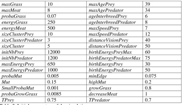
Even if the complexity of this algorithm is not high, in practice this simulation is intensively computationally expensive. As, in general, S is at least three orders of magnitude smaller than N, the dominant part is the computation of the new species. In our first experiments, the simulation manages up to 400,000 individuals and up to 500 species at a given time step, leading to a computational time of over forty minutes for one time step. Therefore our longest simulation until now has been running for two and a half months, corresponding to 7,112 time steps9. As it is the most complete run that we have currently obtained, we consider this run for the discussion in this section. The parameters used for this run are given in table 3. The initial FCM for preys uses table 1 and the initial FCM for predators uses table 2.

The first important thing to notice is that, even if this simulation is a very complex and large adaptive system, the whole behavior of the ecosystem is relatively stable and present interesting correlation patterns. Moreover, having tested numerous different sets of initial parameters, we have noticed that the overall behavior of the simulation is stable, which means that the same phenomenon of epochs of correlated inflation and deflation of the number of individuals, of species, of resources, appears systematically (see section 4.2). As it is a complex dynamic system, even if there are such regularities, the simulation is far from being easily predictable10. The amplitude and time of inflation and deflation vary considerably, but their mutual correlation is conserved.

maxGrass 10 maxAgePrey 39 maxMeat 8 maxAgePredator 34 probaGrass 0.07 ageInterbreedPrey 6 energyGrass 250 ageInterbreedPredator 8 energyMeat 500 maxSpeedPrey 7 sizeClusterPrey 10 maxSpeedPredator 12 sizeClusterPredator 3 distanceVisionPrey 40 sizeCluster 5 distanceVisionPredator 50 initNbPrey 12000 birthEnergyPreyMax 60 initNbPredator 1200 birthEnergyPredatorMax 75 maxEnergyPrey 650 birthEnergyPrey 30 maxEnergyPredator 1000 birthEnergyPredator 50 probaMut 0.005 minEdge 0.075 Mut 0.15 highMut 0.2 SmallProbaMut 0.001 growGrass 0.8 probaGrowGrass 0.0085 decreaseMeat 1 TPrey 0.75 TPredator 0.7

Table 3. Initial parameters of the simulation

4.2 Overall analysis of the simulation

9 _{The current implementation of the simulation is written in C# and has been running on an AMD Athlon}

64 X2 Dual 4200+ processor with 4GB of memory.

10 _{There is no way, excluding the simulation itself, to predict the state of the system at time step t knowing}

What is very useful for a biological interpretation with such detailed simulation is that all the parameters of all components remain accessible at any time in the evolving process. We have, for example, access to general parameters describing our population such as the current number of individuals and food units, the number of agents doing each type of action, the average energy level of individuals, the average current age of individuals, the average age of death of individuals, the average and maximum number of interbreeding by individual, etc. We also have access to the average value of the activation level of all concepts of the individuals, to the current number of species and for each species we have access to its average matrix. We could even have access to the speciation events and then construct the complete exact phylogeny of the evolving predator and pray species. To illustrate the behavior of the simulation and to see if it has properties that are known to exist in ecosystems, we have extracted several of these parameters and we have also computed the cross correlations between them. As these correlations may not be in phase (for example the number of predators at a given time step will have an influence on the number of preys several time steps later) and that this difference of phase is unknown and can differ for every couple of parameters, we have computed the maximum cross correlation value by shifted one time series against the other using the Pearson formula:

with x(i) the value of the time series x at time step i, d the shift value, y(i-d) the value of the time series y at time step i-d and mx (resp. my) the average value of the time series x (resp. y). We present the results in table 4 and 5. Several of the cross correlation coefficients are very high such as between the number of preys and the number of eat actions for prey (0.98), the number of preys and the number of breed actions for preys (0.99) or the number of socialize actions and breed actions for predators (0.94). For these cases, it seems that there is a direct correlation between the number of individuals and the number of individuals choosing an action, which means that an almost constant proportion of individuals choose this action during the whole simulation. For others, even if the correlation coefficient is quite high, the phenomenon is more complex. We selected several of them and presented and discussed their correlated evolutions11. In figure 4, 5, 8, 9, 16 and 18 it should be notice that there exists cycles in the correlations between several parameters. This phenomenon clearly illustrates the fact that most of the parameters follow an oscillatory pattern. Long term correlations (high values of d) thus represent correlations between two different cycles of the oscillatory patterns of two parameters.

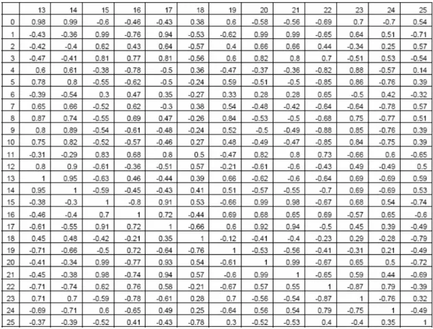
Table 4. Value of the maximum cross correlation for 26 parameters with a shift -2500 < d < 2500. A cell of coordinate (x,y) corresponds to the highest cross correlation between x and y with 0 ≤ d ≤ 2500 if x < y and with -2500 ≤ d ≤ 0 if x > y. The parameters are: (0) number of preys, (1) number of predators, (2) number of prey species, (3) number of predator species, (4) grass level, (5) meat level, (6) prey average energy, (7) predator average energy, (8) escape, (9) search food for prey, (10) socialize for prey, (11) explore for prey, (12) wait for prey, (13) eat for prey, (14) breed for prey, (15) hunt, (16) search food for predator, (17) socialize for predator, (18) explore for predator, (19) wait for predator, (20) eat for predator, (21) breed for predator, (22) foe close, (23) satisfaction for prey, (24) prey close, (25) satisfaction for predator.

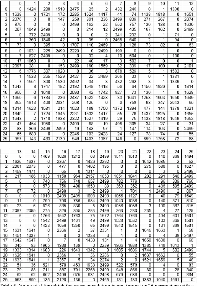
Table 5. Value of d for which the cross correlation is maximum for 26 parameters with a shift -2500 < d < 2500. The parameters are the same as in table 4.

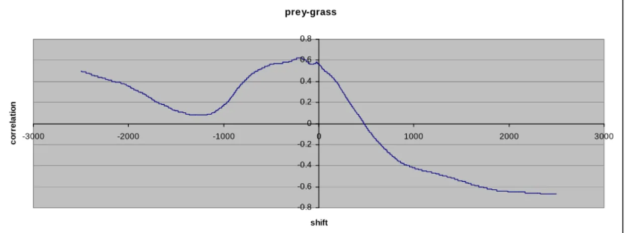
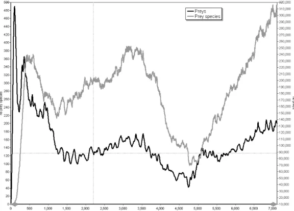
In figure 3, the correlated evolution of the number of preys, the number of predators and the number of grass units are presented for the whole simulation (7,112 time steps). As we should expect with a predator-prey system, it is clear that there is a dependency between the number of preys and the number of predators. The evolution of the number of predators follows the one of preys and vice-versa. When the number of preys grows, the number of predators also grows few time steps later. But when the number of predators grows too much, the number of preys decreases few time steps later, leading to a new later decrease in the number of predators. The maximum cross correlation value between the number of preys and predators is -0.57 for d = 1424. But since there is a third entity, the number of grass units involved in this interacting system, its level influences the other two. The maximum cross correlation between the number of preys and the level of grass is -0.67 for d = 2475. The figures 4 and 5 show the variation of these two cross correlations for all values of d. It appears that the correlation between the number of preys and the number of predators is much more complex that the one between the number of preys and the level of grass. By studying figure 3 we can see that after the time period from time step 1 to 250, in which the number of preys is very high, the number of grass units decreases very fast until time step 1,725. During this period there is also a high decrease in the number of preys. Then it takes a long time to recover from this situation and the number of preys and grass units do not reach such a high level anymore. It is the union of the phenomena of high number of predators and low number of preys that allows a fast growth of grass between time steps 3,550 and 4,750. Then, as the number of predators decreases and the number of grass units is high, the population of preys enters a period of very fast growth, which in turn leads to an increase in the number of predators and a decrease in the number of grass units.

Figure 3. Evolution of the number of individual preys, the number of individual predators and the number of grass units

prey-pred -0.7 -0.6 -0.5 -0.4 -0.3 -0.2 -0.1 0 0.1 0.2 -3000 -2000 -1000 0 1000 2000 3000 shift co rr e lat io n

Figure 4. Cross correlation between the number of preys and the number of predators for -2500 ≤ d ≤ 2500. prey-grass -0.8 -0.6 -0.4 -0.2 0 0.2 0.4 0.6 0.8 -3000 -2000 -1000 0 1000 2000 3000 shift co rr e lat io n

Figure 5. Cross correlation between the number of preys and the level of grass for -2500 ≤ d ≤ 2500.

Figures 6 and 7 illustrate the correlation between the number of individuals and the number of species for each type of individual. In figure 7, it appears that12 the number of predator species is closely correlated to the number of predator individuals. The maximum cross correlation is 0.87 with d = 172. This correlation is also strong for the number of prey species and the number of prey individuals but with a higher difference in the amplitude of the fluctuations. The maximum cross correlation is 0.45 with d = 280. Figure 8 and 9 show that the correlation is much stronger between the number of predators and the number of predator species than between the number of preys and the number of prey species. For each of them the number of individuals increases before the number of species increases. This kind of correlation is what should be expected in an

12

There is in fact a latency delay, between time step 1 and time step 128, needed for some offspring to have evolved enough in comparison to the initial matrix and then for the first species to emerge.

ecosystem. Several publications on existing organisms’ populations show correlation patterns between the number of individuals and the number of species [31]. The difference for these publications is that the data come from different spatial locations since it is very difficult to collect data on the number of individuals and the number of species during a long period of time.

The species-area scaling relation is a classical ecological pattern. Its underlying intuitive idea is: if individuals are collected in different zones, the bigger the sampled area, the more species we find. This relation is used for example in conservation biology, in order to estimate the effects of the size of a reserve on species diversity. More significantly, species-area relations are the fundamentals of the theory of island biogeography [19]. Actually, islands in an archipelago provide ecologists with natural sampling habitats of varying sizes, but with similar environments. When species’ richness is calculated for habitats of increasing size (such as islands), the following scaling relation holds: S = cAz, where S is the total number of species found, A is the size of the sampled area, and c and z are regression constants13. This relation is empirically well supported [8, 19, 27], and the value of z is often around 0.25 for small scale ecological communities. However, no satisfying explanation of the underlying mechanisms of this phenomenon has been proposed yet [8]. Note also that exceptions to the species-area relation have been presented, e.g. in [28], and that the value of z can be greater than 0.25 when sampling large scale and complex areas characterized by greater habitat heterogeneity [19]. In figures 10 and 1114, we present graphs between the log of the number of individuals and the log of the number of species but for our evolving populations (different time steps). The linear dependency between the log of the number of predators and the log of the number of predator species is particularly clear with a slope of 0.99, which is higher than the 0.25 expected but controversial. Even if it is less convincing for preys, the phenomenon is still visible on figure 11.

13 _{On the logarithmic scale, the following equivalent linear relation holds: log(S) = zlog(A) + log(c).} 14 _{As the speciation process takes time to get stabilized, the data presented in these figures correspond only}

to the time steps between 1200 and 7112 for the preys and to the time steps between 1,600 and 7,112 for the predators.

Figure 6. Evolution of the number of individual preys and the number of prey species

Figure 7. Evolution of the number of individual predators and the number of predator species

prey-prey species -0.5 -0.4 -0.3 -0.2 -0.1 0 0.1 0.2 0.3 0.4 0.5 -3000 -2000 -1000 0 1000 2000 3000 shift c o rr el at io n

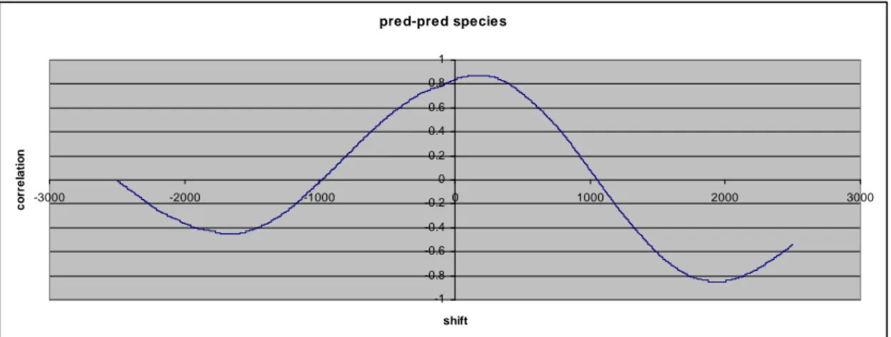
Figure 8. Cross correlation between the number of preys and the number of prey species for -2500 ≤ d ≤ 2500. pred-pred species -1 -0.8 -0.6 -0.4 -0.2 0 0.2 0.4 0.6 0.8 1 -3000 -2000 -1000 0 1000 2000 3000 shift co rre la ti o n

Figure 9. Cross correlation between the number of predators and the number of predator species for -2500 ≤ d ≤ 2500.

Predators (1600 - 7000) 6.0 6.5 7.0 7.5 8.0 8.5 12.0 12.2 12.4 12.6 12.8 13.0 13.2 13.4 13.6 13.8 14.0 Log2 (Predator) L o g 2 ( P red at o r sp ec ies)

Figure 10. Correlation between the number of individual predators and the number of predator species. Slope 0.99

Preys (1200 - 7100) 6.5 7.0 7.5 8.0 8.5 9.0 15.1 15.3 15.5 15.7 15.9 16.1 16.3 16.5 16.7 16.9 17.1 Log2 (Prey) L og2 ( P re y s pec ies )

Figure 11. Correlation between the number of individual preys and the number of prey species. Slope 1.22

Figure 12 presents the overall evolution of the populations of preys and of predators in term of complexity of the behavioral model. The average number of edges in the Matrix L of both populations of preys and predators is computed at each time step. This average value grows almost monotonically for both populations, with a higher slope for predators. As a higher number of edges in a matrix also increases the energy used by the individuals at each time step, it appears that there is enough interest in adding new influence edges between concepts and then to have a more complex behavioral model to compensate for the loss of energy. It is a very interesting result since it shows the interest of the FCM as a behavioral model. The FCM behavioral model is sophisticated and useful enough for the agents (it provides the agents with an efficient way to survive and to propagate their genomic information through generations) to such an extent that a gain in behavior complexity is enough to compensate for the loss of energy. It shows also the capability of this simulation to test some evolutionary hypothesis such as showing how more complex behaviors, even with the associated drawback of an increase in energy needs, could lead to organisms with better abilities to survive and to transmit their genetic information. The number of preys is also plotted in this figure to show the correlation with the number of edges. From time steps 4,750 to 5,100 the prey population grows very fast. The average number of edges for preys grows much faster also during this period. The acceleration in the increase in the number of edges for preys begins around time step 4,450, which is before the acceleration in growth of the population of preys. This could be explained by the fact that mutations in some individuals allow one or more well adapted species to emerge and, after few generations, trigger the growth acceleration of the population of preys event. This hypothesis is strengthened by the fact that this phenomenon is also correlated to a decrease in the number of prey species from time steps 4,550 to 4,800 (the most efficient species dominate) and then to an increase in this number from time steps 4,800 to the end of the simulation (the most efficient species lead to the emergence of new efficient species).

Another analysis that can be performed is the study of the evolution of the average activation level of the concepts of a population. For example, in figure 13, we focus on the activation levels of the action concepts explore and wait of preys and we correlate their evolution with the total number of preys. The maximum cross correlation between the number of preys and the activation level of explore for prey is -0.41 for d = 1330 and the maximum cross correlation between the number of preys and the activation level of wait for prey is -0.41 for d = 0 and d = -6. These two coefficients are not very high and thus show that a more complex interaction should be involved. The activation level of

explore grows very fast at the beginning of the simulation and then remains almost

constant until the end. For the activation level of the wait concept, there is a low and constant decline from the beginning of the simulation to the time step 1,550. Globally, the activation level of explore is much higher than the one of wait during the whole simulation. The period of fast growth of the population of preys from time steps 4,750 to 5,100 corresponds to a growth of the activation level of wait and explore as well, but after time step 5,100 the activation level of wait tends to grow slowly and the activation level of explore to decrease slowly. It seems that the explanation given for figure 12 about important mutations that change the efficiency of prey species after this time step can also explain the change in behaviour observed with the change in the level of activation

of the wait and explore concepts. Noticing that the number of grass units and the overall number of preys are relatively high during this period, the exploration behaviour could be less interesting and the wait behaviour, avoiding too much energy consumption, could be more attractive.

Figure 12. Evolution of the number of individual preys, of the number of edges in the prey FCM and of the number of edges in the predator FCM.

Figure 13. Evolution of the number of individual preys, of the number of preys choosing the explore action and of the number of preys choosing the wait action.

Figure 14 shows that very different patterns of evolution of behaviors can emerge. The number of predators choosing the hunt action follows almost exactly the number of predators (the maximal cross correlation is 0.99 for d = 0 and d = 8) whereas the evolution pattern of the number of predators choosing the searchForFood action vary considerably from the one of the number of predators. The maximal cross correlation is -0.76 for d = 2367 but also 0.71 for d = 0 showing that there is an overall quite good correlation between the searchForFood action and the number of predators. It seems that the action of hunting is constantly important during the whole simulation. Approximately the same fraction of the whole predator population chooses the hunt action at each time step. For the searchForFood action, this is not the case. At the beginning of the simulation a very small fraction of the predators choose this action. Then the number of predators choosing the searchForFood action grows almost constantly until the time step 3,650, even when the overall number of predators highly decreases. This can be explained by the fact that the evolutionary process allows the predators to discover the importance of searching for food to take advantage of the available food units (generated by the large amount of preys dying of lack of energy or of old age) in the world. After this maximum, the number of predators choosing to search for food decreases with the total number of predators but with a much lower slope, and then stabilizes even when the number of predators grows very fast from time step 4,950 to the end of the simulation. This final phenomenon does not seem to be correlated to the number of meat units available since this number tends to grow at the end of the simulation (data not shown).