Oil, metals and minerals : World prices and Quebec’s regions (Results from a CGE model)

(1)

1 Centre INRS-UCS, Institut national de la recherche scientifique, Montréal 2 Université Laval, Québec, and independent researcher

Oil, metals and minerals :

World prices

and Quebec’s regions

(Results from a CGE

model)

André Lemelin

1

and Véronique Robichaud

2

(2)

Except where otherwise noted, this work is licensed under http://creativecommons.org/licenses/by-nc-nd/3.0/

(3)

SUMMARY

The authors have developed a computable general equilibrium (CGE) model of the province of Quebec, based on a new, relatively detailed social accounting matrix (SAM) for 2011. From the whole-Quebec SAM, they elaborated a multiregional SAM using, in particular, regional data produced by Institut de la statistique du Québec (ISQ), most notably estimates of regional GDP by industry. The two SAMs stand out for the care that was taken in conceiving their structure, and then in quantifying its elements from publicly available data, completed with information from various sources, proportionality assumptions and bi-proportional adjustments (RAS technique), subject to accounting identities and benchmark data. Quebec is broken down into 16 analytical regions: the Montreal census metropolitan area (CMA), subdivided in three (Montreal, Laval, Rest of the CMA); the 5 other CMAs in Quebec; 6 other analytical regions, called “peri-metropolitan”, non-metropolitan parts of the administrative regions (AR) having territory in common with each CMA; finally, two peripheral regions, Rest-of-the-North and East. Interregional trade flows were generated from regional output–domestic demand balances using a gravity model.

The multiregional model built on the basis of that SAM, MEGBEC, is unique in Quebec. It is a recursive dynamic model inspired from PEP-1-t, considerably modified to take full advantage of the wealth of available data and adapt it to the specific structure of the Quebec economy. The MEGBEC model is used here to simulate the impact on Quebec regions of the drop in world prices of oil and metals and minerals. Results show that the fall in oil prices has a positive but diffuse effect on the Quebec economy, while the drop in the prices of metals and minerals has a negative impact and hits regions unequally: regions where mining and primary metal manufacturing are concentrated are hardest hit. Combining both shocks had a slightly positive overall impact, but a negative one in regions dependent on the prices of metals and minerals.

(6)

OIL, METALS AND MINERALS :

WORLD PRICES AND QUEBEC’S REGIONS

(RESULTS FROM A CGE MODEL)

1. Introduction

The multiregional computable general equilibrium (CGE) model MEGBEC is unique: to our knowledge, there is no other multiregional CGE model of Quebec; there is not even a multiretional input-output model. The model distinguishes 16 so-called “analytical regions” (ANAR). These regions were delineated in Lemelin (2013)1_{to define geographical entities that are economically meaningful and cover the whole}

territory, while taking into account available economic data sources. Now, economic data published by Institut de la statistique du Québec relate either to census metropolitan areas (CMAs) – and then all the rest of the province is aggregated as “non-metropolitan” –, or to “administrative regions” (ARs) – not suitable for economic analysis. By combining data relating to CMAs and ARs using addition and subtraction, it is possible to define regions in such a way that the organic character, so to speak, of CMAs is maintained, but non-metropolitan areas are not lumped together. Appendix 3 provides a map and a definition of the analytical regions. Each of the six CMAs is an analytical region, except the Montreal CMA, which is subdivided in three, a refinement made possible by the fact that the ARs of Montréal (Montreal island) and Laval are completely embedded in the CMA. Six other analytical regions, which we call “peri-metropolitan” consist of the non-metropolitan parts of the ARs having territory in common with the CMA. Finally, we have defined two peripheral regions, Rest-of-the-North and East. Admittedly, this geographical breakdown is not ideal for economic analysis. But it is a realistic compromise which, as we intend to show, makes it possible to obtain enlightening results.

The MEGBEC model is based upon a rather detailed social accounting matrix (SAM), with 44 industries, 64 products, 4 production factors and 20 economic agent accounts (Appendix 2).2_{The version of the}

model which we present here is operational, but somewhat like a freshly launched ocean liner, it floats and can sail, but not all of its superstructure is in place.

The issue we want to examine is related to recent economic developments, in particular, the fall in the prices of oil, and of metals and minerals. Oil-producing provinces in Canada have been hard hit by the crude oil price collapse, but the same may have benefitted oil-importing provinces such as Quebec. On

1 It is likely that others have used the same geographical breakdown.

2 To our knowledge, there are only two other CGE models of Quebec: the Quebec Ministry of Finance model, not open to use by researchers, and a model developed by the Groupe de Recherche en Économie et Développement International (GREDI) of the Université de Sherbrooke. See the corresponding section regarding other Quebec CGE models in the list of references.

(7)

the other hand, the euphoria of the raw materials boom has given way to a slump which has left behind the Plan Nord of the Quebec government. Of the two shocks, one positive, the other negative, which have hit the Quebec economy, we try to see which one dominates, and how the impact varies from region to region.

The rest of this paper is organized as follows. In Section 2, we describe how the SAM has been elaborated, a task which was accomplished over a fifteen-month period, with very modest means. Section 3 presents the model, evolved from the PEP-1-t model, but nonetheless markedly different. In Section 4 the basic scenario and the simulation scenarios are defined, and the results are analysed. Concluding remarks complete the article.

2. Elaboration of the social accounting matrix

The SAM underlying the model was elaborated in two phases. We first built a SAM for Quebec as a whole, the general structure of which is illustrated in Appendix 4 using an aggregated table. The SAM represents transactions flows in the economy following the format put forward in the United Nations national accounting system (INTER-SECRETARIAT WORKING GROUP ON NATIONAL ACCOUNTS,2009)3.

Once completed, the SAM of Quebec as a whole was treated as a benchmark for the regional SAMs. The latter were developed using a combination of regional data and regional allocators to distribute SAM values among the regions.

We now proceed to present a brief account of the very involved process of SAM construction.

2.1ELABORATION OF THE SAM FOR QUEBEC AS A WHOLE

The SAM for Quebec as a whole was elaborated from the input-output (IO) tables4_{for Quebec in 2011,}

produced by the Industry Acounts Division of Statistics Canada. The provincial IO tables have confidential entries, which have been reconstituted using corresponding data for Canada and applying the minimum cross-entropy method (RAS technique).

Moreover, the publicly available IO tables are at the S-aggregation level, where all manufacturing is lumped together. Using various information sources, proportionality assumptions, and bi-proportional adjustments (RAS technique), it was possible to disaggregate manufacturing into 19 industries. The main source of information was CANSIM Table 381-0031, which presents provincial gross output by sector

3 Regarding the general structure of the SAM and the national accounting concepts, the interested reader is referred to Decaluwé et al. (2013b).

(8)

and industry. We have also used results from the Quebec input-output model (Modèle intersectoriel du Québec – MISQ), which were available on the Institut de la statistique du Québec website for awhile. At this stage, the tables are at basic prices, that is, without taxes on products or transport and trade margins. The balanced final and intermediate demand tables were revalued at market prices (“purchasers’ prices” in Statistics Canada terminology), using corresponding Statistics Canada tables; and the SAM margin accounts were created. Finally, the SAM was adjusted to be exactly in line with the Quebec income and expenditure accounts (Comptes économiques des revenus et dépenses du Québec) published by the Institut de la statistique du Québec on the basis of Statistics Canada data.

From that initial SAM, several improvements have been applied.

First, given that mixed income (also called “Net income of unincorporated business”) includes factor payments to capital and to labor, we have separated the two by subtracting the employment income of self-employed workers, according to CANSIM Table 383-0031. This will make it possible, when using the model, to take into account, at least partly, the expanding role of self-employment in the labor market. Secondly, we have estimated property income paid and received by economic agents (interest, dividends, etc., all treated as transfers in the national accounts), using available data for Quebec and completing from data relating to Canada, with proportionality assumptions. For want of information regarding property income cross-flows between Quebec and the rest of Canada (RoC), we made the hypothesis that Canada is financially fully integrated, without friction; that seems to be less restrictive than assuming no cross-flows. So we imputed cross-flows between Quebec and the RoC applying bi-proportional adjustment to property income flows, subject to incomes paid and received and estimated flows relating to the rest of the world (RoW). Such “audacity” is justified by the fact that under standard modeling, property income received from the RoC would be exogenous and fixed, while that paid to the RoC would be proportional to the payer’s income, or at least would be endogenous. If, as we believe, financial income cross-flows between Quebec and the RoC are large, ignoring them in simulations would grossly under-estimate changes in the amounts of property income paid to the RoC by Quebec’s economy.

Thirdly, to take advantage of the fact that capital stock and investment expenditures are detailed by asset category, on the basis of CANSIM Table 031-0005, the rate of capital depreciation in each industry is a weighted average of the depreciation rates of the assets that make it up.5

5 We had hoped to better take into account the different depreciation rates. Alas, the composition of investments and that of the capital stock according to Table 031-0005 are different from one another, and we could not reconcile them using an investment model that would have taken account the various speeds at which assets depreciate. For that, the composition of the capital stock would have to evolve from period to period, and we didn’t have enough time to develop the corresponding model.

(9)

Lastly, once we had estimated the capital stock and investment expenditures of public sector industries (Appendix 2, industries 40 to 44) by asset category, we extracted stocks of, and investment in road infrastructures.6_{Introducing that distinction makes it possible, in particular, to reproduce observed public}

investment expenditure patterns without adding the infrastructure capital to the productive capital directly related to the activity of public sector industries. Eventually, it will be possible to conduct studies of the impact of infrastructures along the lines of Bahan et al. (2011) and Boccanfuso et al. (2014a and b).

2.2ELABORATION OF THE MULTIREGIONAL SAM

The multiregional SAM consists of 16 SAMs in a diagonal, to which are added 23 supraregional acounts, as shown in Figure 1. Each one of the 16 SAMs has the same structure as the whole-Quebec SAM illustrated in Appendix 4, except that some of the agent accounts and the savings-investment accounts are missing. Accounts ISBL (Non-profit institutions serving households ‒ NPISH) and RPROPRI (Property income ‒ interest payments, dividends, etc.) are supraregional accounts. In addition, accounts FED (Federal government), RPC (Canada Pension Plan), PROV (Provincial government) and RRQ (Régime de rentes du Québec) have a supraregional counterpart where regional surpluses and deficits, together with some transfers, are consolidated. Accounts RdC (Rest-of-Canada) and RdM (Rest-of-the-World, outside Canada) bring together exports and imports of all regions. Finally, supraregional account RdQ (Rest-of-Quebec) gathers imports of all regions from other Quebec regions, and their exports towards other regions in Quebec; interregional flows are contained in separate tables, one per product.

6 Sources used are CANSIM Tables 031-0004, 381-0023 and 381-0031, as well as the following reports: Applied Research Associates (2008), Deloitte&Touche (2012) and Ministère des transports du Québec (2012).

(10)

Figure 1 – Layout of the multiregional SAM

2.2.1 GDP by region and by industry

To assemble regional SAMs, and then a multiregional SAM, we first used data on regional GDP by industry published by ISQ.7_{These data are published by administrative region (AR), and by census}

metropolitan area (six CMAs and non-metropolitan Quebec). They were combined by adding and subtracting to obtain GDP by industry for each analytical region (ANAR; see Appendix 3).

Given their level of detail, these tables inevitably have confidential cells. Missing values have been estimated separately for ARs and CMAs from sums of missing values in each industry for all regions, and in each region for all industries, applying a relevant a priori distribution and the RAS adjustment technique. Estimation proceeded by blocks of industries, then the results were combined for each ANAR. For manufacturing, some indicators have been drawn from Statistics Canada’s Annual Survey of Manufacturing and Logging Industries.

2.2.2 SAM

Next, GDP by industry and by ANAR was used as an allocator for IO data (intermediate demand for products and output). Household consumption was distributed among ANARs in proportion to ISQ’s regional disposable income, which is tantamount to assume that the average propensity to consume is uniform, and that the structure of consumption expenditures is everywhere the same. Final demand by

7 On ISQ’s regional GDP estimation method, see Lemelin and Mainguy (2009a, 2009b et 2008).

MCS ANAR-01 MCS ANAR-02 MCS ANAR-16 Supraregional accounts Supra-regional accounts

(11)

NPISHs was allocated to regions according to the amount of transfers from households to NPISHs. Final demand by public administrations (industries 40-44) is given by the value of their industry outputs for all levels of government taken together. Regarding investment expenditures, we used ISQ-published data on capital and repair expenditures from Statistics Canada’s Annual Capital and Repair Expenditures Survey, supplemented with building-permits data. Intermediate and final demand estimated in that way was then converted to market prices assuming that margin rates and the rates of taxes on products are uniform across Quebec.8

Wages and mixed income received in each ANAR are calculated using ISQ data on disposable income by region. The discrepancy between wages received and paid according to value added by industry was attributed to commuting and shifted to a supraregional account. Corporate capital income and capital consumption expenditures (depreciation) are transferred to supraregional accounts SOC (Corporations) and INV (accumulation) respectively. The incomes of local administations (including school boards) were distributed among regions using allocators constructed from data of the Ministère des affaires municipales et de l’occupation du territoire (MAMOT), except for transfers received from the Provincial government (essentially, school board funding), which have been allocated according to public expenditures on education. Household income taxes are drawn from ISQ regional personal income data, assuming constant federal and provincial tax shares. Household transfers to NPISHs and to the RoW, as well as transfers received by households (except property income received from corporations) are also taken directly from ISQ regional personal income data. The rest of transfers has been established by applying proportionality rules, subject to accounting identities.

The previously established final demand of public administrations was disaggregated by level of government, either according to proportions in the whole-Quebec SAM, or using employment and salary data from Statistics Canada (CANSIM), the Federal and Quebec Treasury Boards, and, for local government, MAMOT.

2.3ELABORATION OF INTERREGIONAL TRADE FLOWS

After building the regional SAMs, regional domestic production and demand for each product is known. The difference is the region’s net exports. But regional data contains no information on crosshauling, regarding neither the origin of regional imports, or the destination of regional exports. Regional science literature is replete with writings about that difficulty, and there exists a large number of non-survey methods to construct exchange flows on the basis of different models.

8 We reckon that the assumption of uniform transport margin rates is not realistic. We have accepted it for the time being, for want of indicators that would allow to modulate them according to geography.

(12)

For our part, we created interregional trade flows using a gravity model. Formally, the problem is, for each product, to fill in an origin-destination matrix whose marginal totals are known from the multiregional SAM. Origin (row) totals are given by regional outputs and by the volume of Quebec’s imports from the RoC and the RoW; destination (column) totals are given by regional domestic demand and Quebec’s exports to the RoC and the RoW.

2.3.1 Gravity model

The gravity model, in its so-called structural form (Head and Mayer, 2015) is summarized in the following equation j i j j i i j i

X

Q

F

,

=

_Ω

_Φ

τ

, [iii001] where

F_i,j: exports from region of origin i to region of destination j

∑

=

i i j

j

F

Q

, : domestic demand in destination region j

∑

=

j i j

i

F

X

, : output (supply) in region of origin i

τ_i,j: Power of attraction between origin region i and destination region j

∑

_Ω = Φ     j

X

j ,

τ

: inward multilateral resistance factor of destination region j

∑

_Φ

=

Ω

   

Q

i

τ

, : outward multilateral resistance factor of origin region i

Variables Φ_j et Ω_i are called “inward multilateral resistance” and “outward multilateral resistance” respectively. Terminologically, it is possible to reconcile the notion of resistance with those of accessibility and market potential. Indeed, if consumers in j have easy access to a large number of suppliers i, competition between the latter will confront each of them to greater resistance than if consumer access to suppliers is less easy. Reciprocally, if producers in i may offer their products on a large number of markets j, then the attractiveness of each market individually will be less. To summarize, the easier access residents have to suppliers, the greater the resistance that confronts each of the latter; and the greater the market potential of producers in a region, the better they can resist the power of buyers. It should be noted that the F_i,j in equation [iii001] represent the solution of a RAS adjustment of the a priori matrix given by the τ_i,j, with X_i and Q_j for target marginal totals; the

X

_i

Ω

_i are the row

(13)

multipliers, and the

Q

_j

Φ

_j, the column multipliers. Since the RAS technique is equivalent to cross-entropy minimization, it follows logically that the distribution corresponding to the F_i,j minimizes cross-entropy relative to the distribution corresponding to the τ_i,j. Formally, let

∑

=

k h h k j i j i

F

_F

f

, , , , [iii002]

∑

=

k h hk j i j i , , , ,

_τ

τ

θ

[iii003]

Then [iii001] is the solution to the problem

(

)

∑

j i i j i j i j fi j ,

f

,

ln

f

, ,

min

,

θ

[iii004]

2.3.2 Application to constructing interregional trade flows

The construction of interregional trade flows comprises several steps.

We have built interregional trade flows by applying a gravity model to Municipalités régionales de comté (MRC)9_{population data and road network distances between MRCs’ principal towns. These are}

completed with data on several cities in Canada and the United States10_{regarding their weight in the}

trade network (population, corrected according to the volume of trade with Quebec), and their distances from each MRC.

First, we calculated flows between nodes of the trade network (principal towns of each MRC and external origin/destinations) using equation [iii001], with the following values:

i

X

Q

=

: weight of node i (population, corrected according to trade volumes) σ σ

τ

=

₋₁

=

_, 1− , ,

1

i j j i j i

d

[iii005]

d_i,j: distance between the principal town of MRC i et of MRC j σ : elasticity of substitution between commodities of different origins

9 In Quebec, there are 103 Municipalités régionales de comté (MRC; literally “Regional County Municipalities”). They are responsible for territorial planning.

(14)

It can be seen from equation [iii005] that the larger elasticity σ, the greater the impediment of distance. With a high value of σ, ratios

τ

_i_,_i

τ

_i_,_j and

τ

_i_,_i

τ

_j_,_i for j ≠ i are large and the attractiveness of locally produced goods for buyers or of local outlets for sellers is much stronger than that of other origins or destinations. Consequently, cross-flows tend to be weak. In other words, if the local product is easily substituted to imports, then there is no reason to incur the cost of distance. That is why, to avoid overstating the importance of crosshauling, we set the value of σ at 2,5.11

The weights of the network nodes have been set according to population. For the MRCs, their weight is equal to their population, multiplied by the ratio of the sum for all commodities of the value of

[Quebec domestic demand + domestic output] over the sum for all commodities of the value of

[Quebec domestic demand + domestic output + imports + exports]

As for RoC and RoW nodes, their population was multiplied by the ratio of the sum for all commodities of the value of

[exports + imports]

with the RoC or the RoW, depending on the case , over the sum for all commodities of the value of [Quebec domestic demand + domestic output + imports + exports]

Next, we aggregated the nodes’ weights and the trade flows constructed with the gravity model among MRCs and with RoC and RoW destinations, according to the geographical breakdown of the model: the 16 analytical regions, the RoC and the RoW. Inward and outward resistance variables Φ_j and Ω_i were aggregated as weighted sums. Finally, the τ_i,j indicators of attractiveness between aggregated regions were obtained by reversing equation [iii001], transposed to flows between the aggregate regions

R k h R k R k R h R h R k h,

_X

_Q

F

,

Φ

Ω

=

τ

[iii006]

where superscript R designates components of the aggregate model. Once the attractiveness factors have been calculated, one can reverse equation [iii005] to obtain synthetic distances between analytical regions:

( )

( 1) 1 1 1 , , ,

1

− − −

=

_σ

τ

σ

τ

R k h R k h R k h

d

[iii007]

11 A higher value would have produced improbable results, because of a distorsion in the trade network caused by the proximity of Gatineau to Ottawa.

(15)

The interregional flow generation model consists mainly of attractiveness factors τh,Rk. Given those attractiveness factors, for each product, we solve the simultaneous equation system given by

R k h R k R k R h R h R k h

X

Q

F

_,

τ

_,

Φ

Ω

=

[iii008]

∑

_Ω

=

Φ

h Rh R h R k h R k ,

X

τ

[iii009]

∑

_Φ

=

Ω

k Rk R k R k h R h ,

Q

τ

[iii010] where R k

Q

: domestic demand in aggregate destination region k (exports to that region in the cases of RoC and RoW)

R h

X

: output (supply) in the aggregate origin region h (imports from the region inthe cases of RoC and RoW)

3. CGE model

The MEGBEC model was developed from the PEP-1-t model (Decaluwé et al., 2013). But PEP-1-t is a generic model, and we have altered it to take advantage of available data, as reflected in the SAM structure described above. A detailed description of the model (equations, sets, variables and parameters) is given in Appendix 1.

One of the features of our model is the distinction between corporations and unincorporated business, which is taken into account in the production structure (see Figure 2).

(16)

Figure 2 : Production structure

…

Production (XST_j,z,t)

Composite value added

(VAC_j,z,t) Aggregate intermediate consumption (CI_j,z,t)

Corporations (VA_{’SOC’,j,z,t}

)

_{businesses (VA}Unincoroporated ’IND’,j,z,t

)

Product 1

(DI_1,j,t) Product 2 (DI_2,j,z,t)

Leontief

CES Leontief

Employees (LD’TRA.EMPL’,j,z,t) Capital (KD’KSOC’,j,z,t)

CES

Capital(KD’KIND’,j,z,t) _(LDSelf-employed _{’TRA.AUTO’,j,z,t}₎

(17)

For want of information regarding the intermediate demand of corporations and unincorporated businesses, we assumed that the structure of intermediate consumption and the ratio of intermediate consumption to value added was the same in both cases. At the top level, therefore, the value of production is split according to a Leontief function into intermediate consumption and composite value added, which is a CES aggregate of the value added of corporations and of unincorporated businesses. Value added of corporations is a CES combination of labor supplied by employees (TRA.EMPL) and corporate capital (KSOC); value added of unincorporated businesses similarly combines the labor of self-employed workers (TRA.AUTO) and the capital of unincorporated businesses (KIND).

Each industry’s output is then split between its different products. Total regional supply of each product is then sold on the different markets: Quebec, RoC and RoW. The volume supplied to the Quebec market is finally distributed among the sixteen analytical regions. That process is represented in the model through a nested CET structure as described by equations 67 to 75 in Appendix 1.

The model is recursive dynamic, and the evolution of productive capacity is determined by the accumulation of production factors through time. The supply of labor in each analytical region is exogenous and follows regional demographic perspectives. The stock of capital, by industry and region, is determined by the stock of capital in the preceding period, minus depreciation, to which are added the preceding period’s investments. New capital created by investment is allocated among industries according to the PEP-1-t formulation, or nearly so. In fact, in PEP-1-t, discount rate (IR) is an endogenous variable that appears only in the calculation of the user cost of capital (equation 118 in Appendix A of Decaluwé et al., 2013b), and it has no other role than to adjust investment demand to preserve the balance between total investment demand and the available financing (savings) for private investment (equation 113). Therefore, in PEP-1-t, there is no link between discount rate IR and the rate or return of capital. Here, we use an equation for the discount rate (equation 117) that ties that variable to the rate of remuneration of capital. The discount rate corresponds to the weighted average of capital rates of remuneration, net of depreciation. Naturally, in so doing, we had to add an extra variable, factor

Φ

t in

equation 116, which plays the part of a rationing factor to maintain the private investment‒savings balance (equation 113).

Investments aiming to increase the productive capacity of the public sector are exogenous, as are investments in road infrastructures. The latter, however, have no role in our model for the time being, in that they contribute to increasing the productive capacity of no industry.12

12 In many models that take into account the contribution of infrastructure to productivity, total factor productivity in the industry production functions depends on the stock of infrastructure.

(18)

Finally, the decomposition of investment among different asset categories (building construction, engineering construction, machinery and equipment...) follows a Leontief distribution, proportional to that of the reference period (equation 119) and total investment by asset category is obtained by adding up demand from all industries (equation 120).

Although individual product supply and demand balances are established at the regional level, most macroeconomic balances are implemented at the provincial level, in accordance with the SAM structure (supraregional accounts). So total investment in the province is determined by total savings (Appendix 1, equation 107), and the sum of regional labor supplies is equal to total labor demand by all industries in all regions (Appendix 1, equation 105). Likewise, exchanges with the rest of Canada and the rest of the World are accounted for at the provincial level, as are the corporations’ account, the NPISH account and the property income account. Also, macro aggregates (GDP, household consumption, etc.) and price indexes are computed both at the regional and provincial levels.

Part of the activities of different orders of government are established at the regional scale: current expenditures on goods and services, investment expenditures, transfers to and from households and revenue from indirect taxation. For higher orders of government (provincial, federal, RRQ and CPP), the balance of regional transactions is transferred to the corresponding supraregional account. At that level, the activities of public administrations consist of the following: transfers to and from businesses (corporations and NPISHs), property income paid and received, and high-order intergovernmental transfers. In the SAM, the resulting balance is in line with the value of each order of government’s savings according to the income and expenditure accounts. Equations 22 to 42 in Appendix 1 describe these relations.

The closure rules we use are quite similar to those of PEP-1-t. Per capita public investment expenditures are fixed in real terms, as are current public expenditures. The total value of investments in each period is endogenous and determined by the sum of savings (our model is “savings-driven”). Prices on external markets are exogenous and fixed. Quebec has two trading partners, the RoC and the RoW, both of which are characterized by fixed prices of imports from, and exports to Quebec; trade volumes adjust according to the Quebec internal prices in relation to these exogenous prices. For the RoW, we have maintained the hypothesis of a fixed current account balance (CAB). Regarding the balance with the RoC, we observe that leaving it free produced results that were less than convincing. As a matter of fact, given that the counterpart of a current account deficit (surplus) is positive (negative) foreign savings, any variation in the current account balance with the RoC results in a change of equal magnitude in total investment.

(19)

Therefore, abiding by the TANSTAAFL principle13_{, we applied the same current account balance rule to}

the RoC as to the RoW: the nominal CAB to GDP ratio is constant. But introducing that extra constraint left the model one free variable short. So we introduced an “exchange rate” between Quebec and the RoC. This variable however is to be interpreted as an overall price ratio between Quebec and the RoC: since RoC prices are fixed, the endogenous Quebec-RoC “exchange rate” represents the overall evolution of Quebec prices relative to prices in the RoC. The rate of exchange with the RoW plays the part of numéraire.14

Model parametrization consists in determining the values of parameters that are consistent with the SAM data. But the SAM does not contain enough information to set all parameters, so that some, called “free parameters”, must be assigned values by other means, generally values are drawn from the literature or econometrically estimated. Here, we have borrowed elasticity parameters from various sources. The tables in Appendix 5 contain the values of the main free parameters.

4. Simulation scenarios and analysis of results

4.1SPECIFICATION OF THE BASIC SCENARIO AND SIMULATIONS

We have not yet developed a proper reference scenario as we have, for example, for model PEP-w-t (Lemelin et Robichaud, 2014). Our simulations are conducted starting from a “neutral” business-as-usual (BAU) scenario, where the supply of labor and some other exogenous variables grow according to regional demographic forecasts (total population by ANAR), without shock. Left on its own, so to speak, the model can run to 2060 and later.15

The goal of the simulations is to study the impact of recent developments in the Canadian and world economies on the economy of Quebec and of its regions. Specifically, we consider the impact of the fall in the prices of basic commodities. Among these, we have selected oil, which Quebec imports as crude for its refineries, and metals and minerals, for their importance in Quebec’s economy (mining, aluminum smelting, Plan Nord...).

The sub-index of metals and minerals in the Bank of Canada’s Basic Commodity Price Index (BCPI) covers: potash, aluminum, gold, nickel, iron, copper, silver, zinc and lead. Corresponding products in the model are 08-MIN_METAL (Minerals and metal concentrates) and 27-METAL_PREM (Primary metal

13 “There Ain’t No Such Thing As A Free Lunch”. Practically speaking, in simulations, if the CAB surplus of Quebec with the RoC diminishes, capital accumulation, and hence growth accelerate.

14 There are other options: see Lemelin (2015).

15 Results concerning such a distant future have no value in our opinion, but we consider the possibility of running the model for so long as a test of its robustness.

(20)

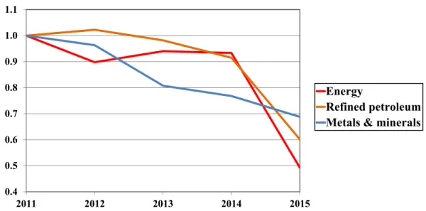
manufacturing). For oil, we have used two price indexes. For product 07-COMBUST (Mineral fuels), we took the Bank of Canada’s BCPI sub-index for energy, consisting in: Crude Oil (WTI, Brent, Western Canada Crude), Natural Gas and Coal. As for product 23-PET_RAFF (Refined petroleum products, excluding chemicals), refining margins partly dissociate the prices of refined products from that of crude oil, so we have built an index from data published by the U.S. Energy Information Administration: we took the twelve-month average of gasoline wholesale and resale price by refiners over all of the United States, for 2011-2015 (last available year).16_{Figure 3 shows the evolution of world prices.}

Figure 3 – Index of basic commodity prices (2011=1.0)

Sources : Bank of Canada (http://www.banqueducanada.ca/taux/indices-des-prix/ippb/)

U.S. Energy Information Administration (http://www.eia.gov/dnav/pet/pet_pri_refmg_dcu_nus_m.htm)

On that basis, we define three scenarios:

• SIM1 : fall in the world prices of energy (crude oil and refined petroleum products); • SIM2 : fall in the world prices of metals and minerals;

• SIM3 : combination of the two preceding scenarios.

4.2SIM1:FALL IN THE WORLD PRICES OF OIL

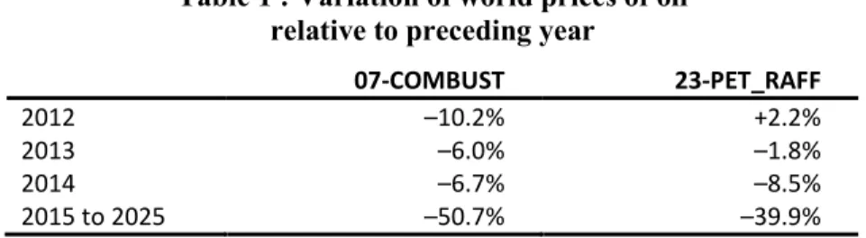
The first simulated shock is a fall in the world prices of crude oil and refined products, both imported and exported. In the model, corresponding products are 07-COMBUST (Mineral fuels) and 23-PET_RAFF (Refined petroleum products). Table 1 describes the evolution of world prices for these products in the simulation.

16 U.S. Total Gasoline Wholesale/Resale Price by Refiners (Dollars per Gallon), Gasoline All grades : http://www.eia.gov/dnav/pet/pet_pri_refmg_dcu_nus_m.htm (site consulté 2016-04-12) 0.4 0.5 0.6 0.7 0.8 0.9 1.0 1.1 2011 2012 2013 2014 2015 Energy Refined petroleum Metals & minerals

(21)

Table 1 : Variation of world prices of oil relative to preceding year

07-COMBUST 23-PET_RAFF

2012 –10.2% +2.2%

2013 –6.0% –1.8%

2014 –6.7% –8.5%

2015 to 2025 –50.7% –39.9%

In order to better understand the impacts, let us first describe the place occupied by these products in the Quebec economy. Demand for product 07-COMBUST is almost entirely fulfilled by imports from the RoW, which represent a little more than 10% of the total value of Quebec’s imports. Even though over 20% of local production is directed to exports (mainly to the RoC), those exports are a negligible share of the total value of Quebec’s exports. So it is expected that a drop in world oil prices essentially benefits importers, with little impact on exporters.

The story is different with refined petroleum products. In fact, Quebec is a net exporter of refined products to the RoC, but a net importer from the RoW. All in all, the value of exports is roughly equal to the value of imports. Nearly half of the output of refined petroleum products is for the export market, and nearly half of demand in Quebec is satisfied from imports. Therefore, a shock to world prices will impact both supply and demand.

On the domestic market, purchases of mineral fuels are mostly for intermediate consumption. The refining industry (15-RAFFIN) by itself accounts for almost 80% of the total demand for product 07-COMBUST. As for refined petroleum, it is also largely for intermediate consumption, in almost every industry, but prominently in transport (close to 18% of total demand) and construction (close to 11%). Household final demand represents almost one third of total demand.

Table 2 : Supply and demand of oil products in Quebec, 2011

07-COMBUST 23-PET_RAFF Demand:

Intermediate demand (M$) 13 246 10 377

Final demand (M$) 106 4 975

Share of intermediate demand 99.2% 67.6%

Supply:

Share of product in the sales of industry 15-RAFFIN 2.4% 96.0%

Both goods are produced by the same industry, 15-RAFFIN. So a drop in world oil prices will have a two-way impact on the refining industry: it will diminish its production costs and, ceteris paribus, the value of its sales.

(22)

Regionally, the refining industry is principally located in the Montreal and Quebec CMAs. But in spite of it all, the relative importance of that industry in value added (GDP) remains small, both regionally and in Quebec as a whole.

4.2.1 Impact on the Quebec economy as a whole

Given that the products involved in the shock account for a greater share of total imports than exports, it is no wonder that the lower world prices of oil improve Quebec terms of trade with the RoW, and even with the RoC, as soon as 2012: the Fisher price index of exports rises relative to that of imports. Consequently, since the balance of trade is fixed in the model closure rules, the volume of exports to the RoW increases less than that of imports as time goes by; and although the opposite happens to the volume of trade with the RoC, the net effect is to free resources.

On the supply side, the fall in oil prices on the export market discourages foreign sales. Produces wanting to redirect their output to the domestic market will need to lower their local sales price. Symmetrically, the lower import price of product 07-COMBUST allows refiners to cut their production costs considerably. The lower price boosts demand, letting producers increase their output somewhat. Production initially directed to international exports is diverted to the domestic market and the RoC.

Table 3 : Impact on the supply of oil products (% variation relative to the BAU scenario, 2025)

Exports to the RoC

Price -56.1 -36.4

Volume -38.2 1.2

Exports to the RoW

Price -59.2 -41.4 Volume -42.2 -5.9 Sales in Quebec Price -40.5 -32.0 Volume -18.4 6.5 Total suply Price -43.4 -34.8 Volume -22.4 2.9

(23)

Table 4 : Impact on the demand for oil products (% variation relative to the BAU scenario, 2025)

Imports from the RoC

Price -46.9 -35.2

Volume -3.8 10.7

Imports from the RoW

Price -50.7 -39.9 Volume 7.6 27.4 Purchases in Quebec Price -40.5 -32.0 Volume -18.4 6.5 Total demand Price -50.0 -34.9 Volume 5.4 12.8

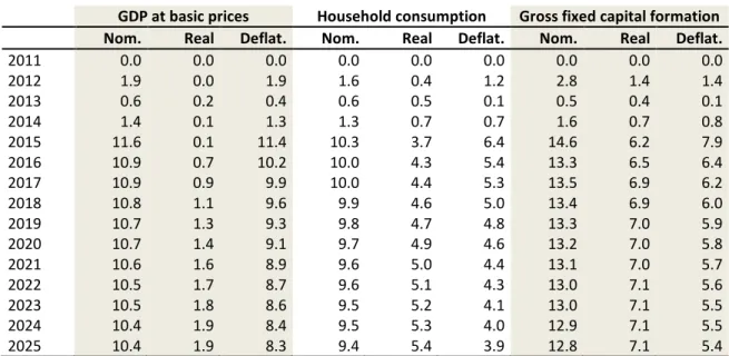
Given that two-thirds of the demand for refined products are used as inputs in other industries, the lower price of oil reduces the cost of inputs in several industries, increasing the share of factor incomes. Lower oil prices also release part of the households’ consumption budget, increasing real consumption. As soon as the first year of the shock (2012), factor incomes rise (+2.4% for capital, +1.6% for labor), household demand increases (+1.6% in nominal terms, +0.4% real terms), and savings by all agents, and consequently investment, go up (+2.8% nominal, +1.4 real).

For 2011 and 2012, real GDP is the same in SIM1 as in the BAU because real GDP is nothing but a measure of the volume of production factors, capital and labor, which is the same in both scenarios for 2011 and 2012. But beginning in 2013, there appears a gap which can only result from a quicker capital accumulation in the SIM1 scenario (the supply of labor is identical in the two scenarios). And indeed, as mentioned in the preceding paragraph, the real value of savings is greater in SIM1 from 2012, so that beginning in 2013, when the new capital created in 2012 comes on line, the capital stock is larger than in the BAU. But how is it that the cost of investment increases less than savings? In fact, a significant share of equipment goods needed for investment is imported; in the simulation, the prices of these goods on the world market is unchanged, while domestic prices rise, so that the investment price index increases less than savings.

(24)

Table 5 : Impact on macroeconomic indicators (% variation relative to the BAU scenario)

GDP at basic prices Household consumption Gross fixed capital formation Nom. Real Deflat. Nom. Real Deflat. Nom. Real Deflat.

2011 0.0 0.0 0.0 0.0 0.0 0.0 0.0 0.0 0.0 2012 1.9 0.0 1.9 1.6 0.4 1.2 2.8 1.4 1.4 2013 0.6 0.2 0.4 0.6 0.5 0.1 0.5 0.4 0.1 2014 1.4 0.1 1.3 1.3 0.7 0.7 1.6 0.7 0.8 2015 11.6 0.1 11.4 10.3 3.7 6.4 14.6 6.2 7.9 2016 10.9 0.7 10.2 10.0 4.3 5.4 13.3 6.5 6.4 2017 10.9 0.9 9.9 10.0 4.4 5.3 13.5 6.9 6.2 2018 10.8 1.1 9.6 9.9 4.6 5.0 13.4 6.9 6.0 2019 10.7 1.3 9.3 9.8 4.7 4.8 13.3 7.0 5.9 2020 10.7 1.4 9.1 9.7 4.9 4.6 13.2 7.0 5.8 2021 10.6 1.6 8.9 9.6 5.0 4.4 13.1 7.0 5.7 2022 10.5 1.7 8.7 9.6 5.1 4.3 13.0 7.1 5.6 2023 10.5 1.8 8.6 9.5 5.2 4.1 13.0 7.1 5.5 2024 10.4 1.9 8.4 9.5 5.3 4.0 12.9 7.1 5.5 2025 10.4 1.9 8.3 9.4 5.4 3.9 12.8 7.1 5.4

In the course of time, growth in the stock of capital makes labor relatively scarcer, and its price rises. Moreover, increased economic activity generates more revenue for governments, and smaller deficits. Savings by corporations and households also contribute to higher total savings. Eventually, the gap between the two scenarios is widened by a feedback effect of growth on investment through RoW savings. Indeed, given that the trade balances with the RoW and the RoC are fixed proportions of GDP at basic prices, and given that their sum is negative (positive external savings), any rise in nominal GDP brings about an increase in foreign savings.

To summarize, our model predicts that the impact of the drop in world prices of crude oil and refined petroleum products will have a positive effect on the economy, even if only microeconomic impacts on resource allocation are taken into account. In a future version of the model, with unemployment, there could be an additional, macroeconomic impact, through a reduction in the rate of unemployment and a move towards full employment of labor.

4.2.2 Regional impacts

The refining industry (15-RAFFIN) is highly concentrated geographically. It generates about 55% of its value added in the Montréal AR (ANAR-01), and close to 27% in the Quebec CMA (ANAR-05). The transport industry (29-TRANSPORT), a prime user of refined petroleum, is relatively concentrated in Montreal (46% of its value added, compared to 34% for all industries taken together).

(25)

Table 6 : Regional impacts

(% variation relative to the BAU scenario, 2025)

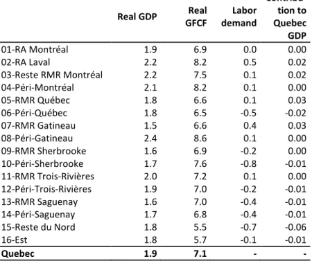
Real GDP _GFCFReal _demandLabor

Contribu-tion to Quebec GDP 01-RA Montréal 1.9 6.9 0.0 0.00 02-RA Laval 2.2 8.2 0.5 0.02 03-Reste RMR Montréal 2.2 7.5 0.1 0.02 04-Péri-Montréal 2.1 8.2 0.1 0.00 05-RMR Québec 1.8 6.6 0.1 0.03 06-Péri-Québec 1.8 6.5 -0.5 -0.02 07-RMR Gatineau 1.5 6.6 0.4 0.03 08-Péri-Gatineau 2.4 8.6 0.1 0.00 09-RMR Sherbrooke 1.6 6.9 -0.2 0.00 10-Péri-Sherbrooke 1.7 7.6 -0.8 -0.01 11-RMR Trois-Rivières 2.0 7.2 0.1 0.00 12-Péri-Trois-Rivières 1.9 7.0 -0.2 -0.01 13-RMR Saguenay 1.6 7.0 -0.4 -0.01 14-Péri-Saguenay 1.7 6.8 -0.4 -0.01 15-Reste du Nord 1.8 5.5 -0.7 -0.06 16-Est 1.8 5.7 -0.1 -0.01 Quebec 1.9 7.1 - -

Having said that, we have seen that the impact of the drop in world energy prices was rather diffuse in the economy between industries, and the same is true geographically: the spatial distribution of economic activity is little changed from the oil price shock. All regions benefit from a rise in GDP beginning in 2013. And, from one region to another, the same industries, roughly speaking, contribute positively or negatively to the SIM1-BAU difference in real GDP.

4.3SIM2:SHOCK ON THE WORLD PRICES OF METALS AND MINERALS

The second simulated shock consists in a drop in the world prices of metals and minerals, both imported and exported. In the Bank of Canada’s BCPI, metals and minerals include: potash, aluminum, gold, nickel, iron, copper, silver, zinc and lead. In the model, these are 08-MIN_METAL (Minerals and metal concentrates) and 27-METAL_PREM (Primary metal manufacturing). Table 7 describes the price shock.

Table 7 : Variation in the world prices of metals and minerals relative to preceding year

2012 -3.7%

2013 -19.3%

2014 -23.2%

(26)

To better understand the impacts of a drop in the world prices of metals and minerals, let us take a look at the place they occupy in the Quebec economy. Seventy-nine percent of the production of industry 05-MINES consists of product 08-MIN_METAL, of which it is the sole producer. That product is 85% exported (39% to the RoC, and 46% to the RoW); on the domestic market, industry 19-METAL_PREM (Primary metal manufacturing) accounts for almost 90% of demand. Product 27-METAL_PREM represents 92% of the output of its principal supplier, 19-METAL_PREM, and it is 77% exported (66% to the RoW, and 11% to the RoC); the domestic market absorbs the rest, half of it as an input for the same 19-METAL_PREM industry. So mining and primary metal manufacturing are by far the industries hardest hit by the drop in the world price of their product. In addition, exports of these two products alone account for nearly 20% of Quebec’s total exports abroad, and nearly 8% of its exports to the RoC. Consequently, a shock on world export prices will also have a strong impact on external trade.17

Table 8 : Supply and demand of metals and minerals in Quebec, 2011

08-MIN_METAL 27-METAL_PREM Demand:

Intermediate demand (M$) 3 140 13 430

Final demand (M$) 129 762

Share of intermediate demand 96.0% 94.6%

Supply:

Share of the product in the sales of industry 05-MINES 78.9%

Share of the product in the sales of industry 19-METAL_PREM 92.4%

The drop in the world prices of metals deteriorates Quebec’s terms of trade with the RoW and even with the RoC as soon as 2012: the Fisher price index of exports falls relative to that of imports. Consequently, the volume of exports increases faster than that of imports as time goes by; the same occurs with the volume of trade with the RoC. It follows that maintaining the current account balances drains more resources.

As expected, exports of metals and minerals decrease markedly, entailing a reduction in production too. Besides, since product 08-MIN_METAL enters in the manufacturing of 27-METAL_PREM, the decline of supply on the domestic market is even greater for minerals. And the world price drop has an impact on the domestic price, which is also more pronounced for minerals than for primary metals.

17 On the import side, almost two-thirds of metals and minerals purchases are imported. But the relative importance of those imports in Quebec’s total imports, around 6%, is much lower than for exports.

(27)

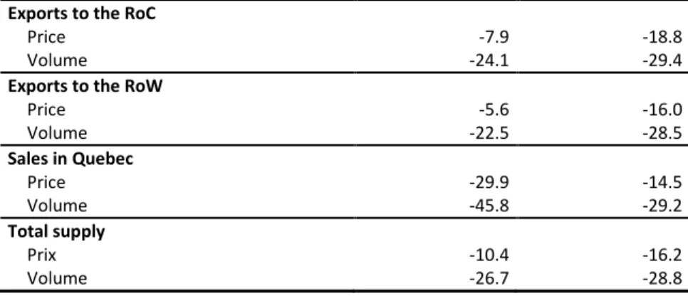
Table 9 : Impact on the supply of metals and minerals (% variation relative to the BAU scenario, 2025)

08-MIN_METAL 27-METAL_PREM

Exports to the RoC

Price -7.9 -18.8

Volume -24.1 -29.4

Exports to the RoW

Price -5.6 -16.0 Volume -22.5 -28.5 Sales in Quebec Price -29.9 -14.5 Volume -45.8 -29.2 Total supply Prix -10.4 -16.2 Volume -26.7 -28.8

The decline in primary metals output results in a fall in the demand for minerals. As shown in Table 10, not only is demand weaker, but producers reduce their domestic purchases in favor of imports which have become relatively less costly. Regarding product 27-METAL_PREM, although the price of competing imports has fallen, the domestic cost of production has benefitted from the drop of minerals prices. So while we observe a reduction in the volume of imports demanded, it is however less than that of the demand for domestic products.

Table 10 : Impact the demand for metals and minerals (% variation relative to the BAU scenario, 2025)

08-MIN_METAL 27-METAL_PREM Imports from the RoC

Price -34.4 -34.4

Volume -1.0 1.1

Imports from the RoW

Prix -31.2 -31.2 Volume -39.5 -4.2 Purchases in Quebec Price -29.9 -14.5 Volume -45.8 -29.2 Total demand Price -32.3 -26.5 Volume -27.2 -13.1

(28)

2011 0.0 0.0 0.0 0.0 0.0 0.0 0.0 0.0 0.0 2012 -0.8 0.0 -0.8 -0.7 -0.1 -0.6 -1.1 -0.4 -0.7 2013 -4.1 -0.1 -4.0 -3.6 -0.7 -2.8 -5.5 -2.2 -3.4 2014 -4.7 -0.3 -4.4 -4.1 -1.0 -3.2 -6.3 -2.8 -3.7 2015 -6.2 -0.4 -5.8 -5.5 -1.3 -4.2 -8.4 -3.8 -4.8 2016 -6.0 -0.7 -5.4 -5.3 -1.3 -4.0 -8.2 -3.9 -4.4 2017 -5.9 -0.8 -5.1 -5.2 -1.4 -3.9 -8.1 -4.0 -4.3 2018 -5.8 -0.9 -4.9 -5.2 -1.4 -3.8 -8.0 -4.0 -4.2 2019 -5.8 -1.0 -4.8 -5.1 -1.5 -3.7 -7.9 -4.0 -4.1 2020 -5.7 -1.1 -4.7 -5.1 -1.5 -3.6 -7.9 -4.0 -4.0 2021 -5.7 -1.2 -4.5 -5.1 -1.6 -3.5 -7.8 -4.0 -3.9 2022 -5.6 -1.3 -4.4 -5.0 -1.6 -3.5 -7.8 -4.0 -3.9 2023 -5.6 -1.3 -4.3 -5.0 -1.7 -3.4 -7.7 -4.0 -3.8 2024 -5.6 -1.4 -4.3 -5.0 -1.7 -3.3 -7.7 -4.0 -3.8 2025 -5.5 -1.4 -4.2 -4.9 -1.7 -3.2 -7.6 -4.0 -3.8

Throughout the 2012-2025 period, a widening gap appears between real GDPs in the SIM2 and BAU scenarios. To summarize, at the 2025 horizon, industries that contribute most to the real GDP gap are the following:

19-METAL_PREM –34.0%

05-MINES –28.4%

07-CONSTRU –18.4%

Together, these three industries represent over 80% of the real GDP loss.

The mechanism whereby real GDP in SIM2 slips away from its BAU level is the same as in scenario SIM1, but reversed. The real value of savings is less in SIM2 than in the BAU scenario, and that slows capital accumulation.

4.3.2 Regional impacts

In our geographical breakdown, the spatial concentration of mining (10-MINES) is very high: it generates 83% of its value added in the large Reste-du-Nord region (ANAR-15), where it is 28% of GDP. As for industry 19-METAL_PREM, it is not concentrated to the same extent as 10-MINES or 15-RAFFIN. But it counts for a substantial share of GDP in some of the regions where it concentrates. That is particularly true in the Saguenay CMA (ANAR-13: 14% of GDP) and in the neighboring region of Peri-Saguenay (ANAR-14: 11%).

Overall, by 2025, all regions suffer a loss of GDP relative to the BAU scenario, even if some of them gain in the beginning (Montreal up to 2017, the rest of the Montreal CMA up to 2016, and a handful of other

(29)

regions in the very early years of the scenario). And, just like in SIM1, it is the same industries which, from one region to another, contribute positively or negatively to the real GDP gap between SIM1 and the BAU.

In spite of the fact that the shock hits some regions (Saguenay, Reste-du-Nord) harder than others, the distribution of Quebec’s GDP among regions is not very different between scenarios, as can be seen in Table 12. Such relative stability is probably partly due to the fact that the preliminary version of the model presented here is better fit for analyzing impacts on production, because income distribution is independent of where production occurs; it follows that no regional impact multiplier comes into play, whether the shock be positive or negative.

Contribu-tion to Quebec GDP 01-RA Montréal -0.59 -2.97 0.45 0.27 02-RA Laval -0.81 -3.58 0.22 0.02 03-Reste RMR Montréal -0.72 -3.23 0.53 0.11 04-Péri-Montréal -1.44 -4.34 0.03 -0.01 05-RMR Québec -0.75 -2.97 0.21 0.05 06-Péri-Québec -1.06 -3.52 0.67 0.01 07-RMR Gatineau -0.48 -2.75 0.08 0.01 08-Péri-Gatineau -0.91 -3.91 0.39 0.00 09-RMR Sherbrooke -0.47 -3.09 0.68 0.02 10-Péri-Sherbrooke -0.81 -3.76 1.00 0.01 11-RMR Trois-Rivières -2.56 -4.85 -0.91 -0.02 12-Péri-Trois-Rivières -0.83 -3.69 0.60 0.03 13-RMR Saguenay -6.65 -9.30 -4.10 -0.12 14-Péri-Saguenay -4.83 -7.92 -2.71 -0.04 15-Reste du Nord -9.11 -12.00 -4.92 -0.34 16-Est -1.35 -3.28 0.04 0.00 Quebec -1.39 -4.04 - -

4.4 SIM3: COMBINED SCENARIO: FALL IN THE WORLD PRICES OF OIL AND OF METALS AND

MINERALS

The question raised in this third scenario is: which of the two shocks has the stronger impact? Will the positive impact of the drop in oil prices overtake the negative impact of the fall in the prices of metals and minerals?

(30)

For Quebec as a whole, the negative effect initially dominates, and increasingly so, until 2015, after which the gap between SIM3 and the BAU scenario becomes positive and growing up to the 2025 horizon, when GDP is about 0.6% higher.

2011 0.0 0.0 0.0 0.0 0.0 0.0 0.0 0.0 0.0 2012 1.1 0.0 1.1 0.9 0.3 0.6 1.7 0.9 0.7 2013 -3.5 0.1 -3.6 -3.0 -0.3 -2.7 -5.1 -1.9 -3.2 2014 -3.3 -0.2 -3.1 -2.8 -0.3 -2.5 -4.8 -2.0 -2.8 2015 5.0 -0.3 5.3 4.6 2.5 2.1 5.7 2.6 3.0 2016 4.6 0.0 4.6 4.4 3.0 1.3 4.7 2.7 1.9 2017 4.7 0.1 4.6 4.4 3.1 1.3 5.0 3.0 1.9 2018 4.7 0.2 4.4 4.4 3.2 1.1 4.9 3.1 1.8 2019 4.6 0.3 4.3 4.3 3.3 1.0 4.9 3.1 1.7 2020 4.6 0.4 4.2 4.3 3.4 0.9 4.8 3.1 1.7 2021 4.6 0.4 4.1 4.2 3.4 0.8 4.8 3.1 1.6 2022 4.5 0.5 4.0 4.2 3.5 0.7 4.7 3.1 1.6 2023 4.5 0.5 3.9 4.2 3.5 0.6 4.7 3.1 1.6 2024 4.5 0.6 3.9 4.2 3.6 0.6 4.7 3.1 1.5 2025 4.5 0.6 3.8 4.2 3.6 0.5 4.7 3.1 1.5 4.4.2 Regional impacts

In the end, regions that loose are those that are directly hit by the shock on the prices of metals and minerals: the Saguenay CMA (‒4.9% relative to BAU), and Reste-du-Nord (‒7.4%), as well as, marginally, the Trois-Rivières CMA (‒0.5%). Roughly speaking, given that industries evolve similarly from one region to another, the fate of regions depends on the industrial composition of their economy.

(31)

Contribu-tion to Quebec GDP 01-RA Montréal 1.47 4.14 0.50 0.26 02-RA Laval 1.52 4.75 0.68 0.04 03-Reste RMR Montréal 1.55 4.37 0.58 0.13 04-Péri-Montréal 0.77 3.99 0.10 0.00 05-RMR Québec 1.14 3.74 0.31 0.08 06-Péri-Québec 0.78 3.08 0.06 0.00 07-RMR Gatineau 1.06 3.87 0.44 0.05 08-Péri-Gatineau 1.48 4.70 0.43 0.00 09-RMR Sherbrooke 1.16 3.83 0.42 0.02 10-Péri-Sherbrooke 0.95 3.85 0.10 0.00 11-RMR Trois-Rivières -0.50 2.38 -0.79 -0.02 12-Péri-Trois-Rivières 1.11 3.41 0.32 0.01 13-RMR Saguenay -4.93 -2.52 -4.33 -0.12 14-Péri-Saguenay -3.06 -1.21 -3.05 -0.04 15-Reste du Nord -7.36 -6.90 -5.52 -0.39 16-Est 0.51 2.48 -0.11 0.00 Quebec 0.64 3.11 - -

5. Conclusion

We have elaborated a 2011 SAM for Quebec, broken down into sixteen analytical regions. We have also generated interregional trade flows by running simulations with a gravity model. On that basis, we have built a multiregional recursive dynamic CGE model, MEGBEC, which can simulate the evolution of the economy of Quebec and of its regions. We have used the MEGBEC model to simulate the impact of recent fluctuations of world prices of oil and of metals and minerals. The simulation results show that a drop in the price of oil has a positive impact on the Quebec economy and benefits all regions in similar proportions. To the contrary, a fall in the prices of metals and minerals has a negative impact on the economy of Quebec as a whole, and the shock is felt differently across regions, with the Saguenay and the North loosing most.

What has been presented here should be considered but a first, albeit major, step in the development of the MEGBEC model. Much has been accomplished, much remains to be done. Among the tasks ahead, let us mention: a tighter link between the remuneration of factors in a region (especially labor), and regional household income; a better specification of the reference scenario; taking account of unemployment on the labor market; modeling the impact of infrastructure investments on the economy; differenciating transport margins over space; expliciting RoC supplies and demands; applying consumption expenditure

(32)

structures specific to each region; taking into account the effect of differences in asset depreciation rates on the of the structure of capital; including welfare indicators... There is still plenty to do!

References

DATA SOURCES

Applied Research Associates, Inc. (2008) Estimation of the representative annualized capital and maintenance costs of roads by functional class, Revised final report TP-14743 submitted to Transport Canada.

http://publications.gc.ca/collections/collection_2009/tc/T22-147-2008E.pdf (access 2016-04-04_

Deloitte&Touche (2012) Étude sur l’état des infrastructures municipales du Québec, diaporama présenté à l’Union des municipalités du Québec.

http://old.umq.qc.ca/uploads/files/content/rapport-complet-infrastructures-municipales-oct12.pdf (access 2016-04-04)

Institut de la statistique du Québec (2014) Comptes économiques des revenus et dépenses du Québec. Édition 2014.

Institut de la statistique du Québec (2014), Perspectives démographiques du Québec et des régions, 2011-2061. tableaux de données diffusés en ligne :

http://www.stat.gouv.qc.ca/statistiques/population-demographie/perspectives/population/index.html (access 2016-03-21)

Institut de la statistique du Québec (2015) Produit intérieur brut (PIB) aux prix de base par région administrative, Québec, 2007-2014, tableau de données diffusé en ligne :

http://www.stat.gouv.qc.ca/statistiques/economie/comptes-economiques/comptes-production/pib_ra_2007-2014.htm

(access 2016-04-04)

Institut de la statistique du Québec (2015) Produit intérieur brut (PIB) aux prix de base par région administrative et par industrie, 2007-2013, tableau de données diffusé en ligne :

http://www.stat.gouv.qc.ca/statistiques/economie/comptes-economiques/comptes-production/pib_industrie_ra_2007-2013.htm

(access 2016-04-04)

Institut de la statistique du Québec (2015) Produit intérieur brut (PIB) aux prix de base par région métropolitaine de recensement (RMR), Québec, 2007-2014, tableau de données diffusé en ligne :

http://www.stat.gouv.qc.ca/statistiques/economie/comptes-economiques/comptes-production/pib_rmr_2007-2014.htm

(access 2016-04-04)

Institut de la statistique du Québec (2015) Produit intérieur brut aux prix de base par région métropolitaine de recensement (RMR) et par industrie, Québec, 2007-2013, tableau de données diffusé en ligne :

http://www.stat.gouv.qc.ca/statistiques/economie/comptes-economiques/comptes-production/pib_industrie_rmr_2007-2013.htm

(access 2016-04-04)

Institut de la statistique du Québec (2015) Dépenses en immobilisation et réparation, régions administratives et ensemble du Québec, 2013-2015, tableau de données diffusé en ligne :

http://www.stat.gouv.qc.ca/statistiques/economie/investissements/prives-publics/ipp_ra.htm (access 2016-04-05)

Institut de la statistique du Québec (2015) Valeur des permis de bâtir selon le type de construction, régions administratives et ensemble du Québec, 2011-2015, tableau de données diffusé en ligne :

(33)

http://www.stat.gouv.qc.ca/statistiques/profils/comp_interreg/tableaux/permis.htm (access 2016-04-05)

INTER-SECRETARIAT WORKING GROUP ON NATIONAL ACCOUNTS (2009). « System of National Accounts

2008 » (SNA2008), Eurostat, International Monetary Fund, OECD, United Nations, World Bank; Bruxelles-Luxembourg, New York, Paris, Washington (D.C.), 662 p.

http://unstats.un.org/unsd/nationalaccount/sna2008.asp

Ministère des transports du Québec (2012) Rapport annuel de gestion 2011-2012

https://www.mtq.gouv.qc.ca/centredocumentation/Documents/Ministere/rapp-annuel/RAG_2011-2012.pdf (access 2016-04-04)

Statistique Canada. Tableau 031-0004 - Flux et stocks de capital fixe non résidentiel, pour l'ensemble des industries, selon les actifs, provinces et territoires

Statistique Canada. Tableau 383-0031 - Statistiques du travail conformes au Système de comptabilité nationale (SCN) par province et territoire, selon la catégorie d'emploi et le Système de classification des industries de l'Amérique du Nord (SCIAN)

Statistique Canada. Tableau 381-0022 - Tableaux d'entrées-sorties, entrées et sorties, niveau détaillé, prix de base, annuel (dollars)

Statistique Canada. Tableau 381-0023 - Tableaux d'entrées-sorties, demande finale, niveau détaillé, prix de base

Statistique Canada. Tableau 381-0028 - Tableaux entrées-sorties provinciaux, entrées et sorties, niveau sommaire, prix de base, annuel (dollars)

Statistique Canada. Tableau 381-0029 - Tableaux entrées-sorties provinciaux, demande finale, niveau sommaire, prix de base, annuel (dollars)

Statistique Canada. Tableau 381-0031 - Production brute provinciale, selon le secteur et l'industrie, annuel (dollars).

Statistique Canada. Tableau 031-0005 - Flux et stocks de capital fixe non résidentiel, selon des industries et actifs, Canada, provinces et territoires, annuel (dollars).

OTHER CGE MODELS OF QUEBEC

BAHAN, David, Alexandre MONTELPARE and Luc SAVARD (2011) An analysis of the impact of public infrastructure spending in Quebec, Cahier de recherche 11-07, Groupe de Recherche en Économie et Développement International (GREDI), Université de Sherbrooke.

BOCCANFUSO, Dorothée, Véronique GOSSELIN, Jonathan GOYETTE, Luc SAVARD et Clovis Tanekou MANGOUA (2014a) An impact analysis of climate change and adaptation policies on the forestry sector in Quebec : A dynamic macro-micro framework, Cahier de recherche 14-04, Groupe de Recherche en Économie et Développement International (GREDI), Université de Sherbrooke.

BOCCANFUSO, Dorothée, Marcelin JOANIS, Mathieu PAQUET and Luc SAVARD (2014b) Impact de productivité des infrastructures : Une application au Québec, Cahier de recherche 15-06, Groupe de Recherche en Économie et Développement International (GREDI), Université de Sherbrooke. BOCCANFUSO, D., M. JOANIS, P. RICHARD and L. SAVARD (2014c) “A Comparative Analysis of

Funding Schemes for Public Infrastructure Spending in Quebec”, Applied Economics, 46(22); 2653-2664.

Oil, metals and minerals : World prices and Quebec’s regions (Results from a CGE model)

Oil, metals and minerals :

World prices

and Quebec’s regions

(Results from a CGE

model)

André Lemelin

and Véronique Robichaud

CONTENTS

SUMMARY

OIL, METALS AND MINERALS :

WORLD PRICES AND QUEBEC’S REGIONS

(RESULTS FROM A CGE MODEL)

1. Introduction

2. Elaboration of the social accounting matrix

X

Q

F

=

Ω

Φ

τ

∑

=

F

Q

∑

=

F

X

∑

X

τ

∑

Φ

=

Ω

Q

τ

X

Ω

Q

Φ

∑

=

F

F

f

∑

=

τ

τ

θ

(

)

∑

f

ln

f

min

θ

X

Q

=

τ

=

=

1

d

d

τ

τ

τ

τ

X

Q

F

Φ

Ω

=

_Ω

_Φ

_Φ

_F

_τ

_X

_Q

_Ω

_Φ