Dataset Optimization for Real-Time Pedestrian Detection

(1)

HAL Id: hal-01566517

https://hal.inria.fr/hal-01566517

Submitted on 1 Aug 2017

HAL is a multi-disciplinary open access

archive for the deposit and dissemination of

sci-entific research documents, whether they are

pub-lished or not. The documents may come from

teaching and research institutions in France or

abroad, or from public or private research centers.

L’archive ouverte pluridisciplinaire HAL, est

destinée au dépôt et à la diffusion de documents

scientifiques de niveau recherche, publiés ou non,

émanant des établissements d’enseignement et de

recherche français ou étrangers, des laboratoires

publics ou privés.

Dataset Optimization for Real-Time Pedestrian

Detection

Remi Trichet, Francois Bremond

To cite this version:

Remi Trichet, Francois Bremond. Dataset Optimization for Real-Time Pedestrian Detection. IEEE

Access, IEEE, 2017, pp.15. �10.1109/ACCESS.2017.2788058�. �hal-01566517�

(2)

ISSN 0249-6399 ISRN INRIA/RR--9084--FR+ENG

RESEARCH

REPORT

N° 9084

2017 Project-Teams STARS

Dataset Optimization for

Real-Time Pedestrian

Detection

(3)

(4)

RESEARCH CENTRE

SOPHIA ANTIPOLIS – MÉDITERRANÉE 2004 route des Lucioles - BP 93 06902 Sophia Antipolis Cedex

Dataset Optimization for Real-Time

Pedestrian Detection

Remi Trichet, Francois Bremond

Project-Teams STARS

Research Report n° 9084 — 2017 — 15 pages

Abstract: This paper tackles data selection for training set generation in the context of near real-time pedestrian detection through the introduction of a training methodology: FairTrain. After highlighting the impact of poorly chosen data on detector performance, we will introduce a new data selection technique utilizing the expectation-maximization algorithm for data weighting. FairTrain also features a version of the cascade-of-rejectors enhanced with data selection principles. Experiments on the INRIA and Caltech datasets prove that, when fine trained, a simple HoG-based detector can perform on par with most of its near real-time competitors.

(5)

Optimisation de Base de Donnée pour la Détection de

Piétons temps-réel

Résumé : Ce document traite de la sélection de données pour la génération de l’ensemble d’entrainement dans le contexte de la détection des piétons en temps-réel grace a l’introduction d’une méthodologie: FairTrain. Apres avoir souligné l’impact des données mal choisies sur les performances des détecteurs, nous allons présenter une nouvelle technique de sélection de données pondéré par l’algorithme d’expectation-maximization. FairTrain propose également une version de cascade-de-rejecteurs améliorée avec des principes de sélection de données. Les expériences sur les bases de données INRIA et Caltech prouvent que, lorsqu’ils sont bien formés, un simple détecteur basé sur des HoGs fonctionne aussi bien que ses concurrents temps-réel.

(6)

Dataset Optimization for Real-Time Pedestrian Detection 3

1 Introduction

Human detection is the keystone of many computer vision applications that depend on the reliability of this important first step. These applications, ranging from surveillance, queue mon-itoring, retail data mining, and automatic pedestrian detection in the automotive industry, have fueled research during the last decade, leading to a soaring number of approaches on the topic.

In a recent study [7], features, context, feature data, and the combination of approaches have been identified as the key performance elements for pedestrian detection. Roughly 30% of approaches focus on developing, combining or adapting features, and this direction has lead to most of the breakthroughs over the past years, such as channel features [20], or convolutional network [48]. Context adaptation [34], harnessing frequent geometry [38][53] or environment patterns [50][69], also successfully received attention from the community, but this algorithm adaptation is often application or even dataset dependent. However, less progress has been stated concerning feature data. Training sets are still generated by applying the same techniques than a decade ago: Increasing the data variability is done by blindly mixing datasets [7], and Bootstrapping [18][30] remains among the preferred choices for training set generation.

In this paper, we argue that data selection and adaptation is an important area that deserves more attention from the community. Training for pedestrian detection is, indeed, a peculiar task. It aims to differentiate a few positive samples with relatively low intra-class variation and a swarm of negative samples picturing everything else present in the dataset. Consequently, the training set lacks discrimination and is highly imbalanced. Due to the possible creation of noisy data while oversampling, and the likely loss of information when undersampling, balancing positive and negative instances is a rarely addressed issue in the literature.

After motivating the need for proper data selection, we will introduce a new training method-ology: FairTrain. Bearing these data selection principles in mind, this system brings up a two-component contribution. First, it harnesses an expectation-maximisation scheme to weight important training data for classification. Second, it improves the cascade-of-rejectors [73][8] classification by enforcing balanced train and validation sets every step of the way, and optimiz-ing separately for recall and precision.

One key aspect of FairTrain is its genericity. It can easily be applied with other features or feature selection methods. Also, it differs from the state-of-the-art data selection methods by its ability to create balanced (training and validation) sets while avoiding over-generalisation. Experiments carried out on the INRIA [18] and Caltech-USA [25] datasets, demonstrate the effectiveness of the approach, leading a simple HoG-based detector to outperform its near real-time competitors.

The rest of this paper is organised as follows. Section 2 reviews the related state-of-the-art. Section 3 gives an overview of the system. Section 4 covers our training set generation technique whereas section 5 details our classification scheme. Section 6 reports our experiments and section 7 concludes on this work.

2 Related Work

Data selection from imbalanced datasets has been a concern for pedestrian detection since the birth of the field. [40] proved that disproportioned datasets degrade SVMs prediction accuracy, especially for non-linearly separable data. Subsequent research on these experiments [70] showed that best performance was obtained for approximately comparable class cardinalities when over-sampling the minority set.

Limited work carries out these issues. Bootstrapping [18][30] is probably the most com-mon adaptation to the problem. This data training mechanism improves accuracy thanks to successive training set updates focusing on samples difficult to classify. It is first initialised on

(7)

4 Remi Trichet, Francois Bremond uniformly drawn negative samples. At each iteration, the negative training set is augmented with the false positives of the previous run. The process keeps repeating until the performance converges or a memory threshold is reached. [62] further showed that 2 iterations lead to optimal performance. [33] adopted a different practice for random forest. They first train t trees with uniformly-drawn samples, use them to obtain harder positive and negative sample to train the next t trees, and iteratively repeat this process. Each tree group bears its own bias, therefore improving the overall forest performance.

Generative techniques consider over-sampling the minority class through artificial data gen-eration. This type of approach suffers from both, over-generalisation and the risk to create erroneous data. The SMOTE algorithm [63] is probably the most renowned one. It creates new data as the linear combination of a randomly selected data point and one of its (same class) k nearest neighbors. Borderline-SMOTE [35] subsequently proposed to improve SMOTE through clever selection and strengthening of weak pairs. ADASYN [36] considered limiting the over-generalisation through density-based data generation. In the same vein, [41] introduced cluster-based oversampling, simultaneously tackling the intra- and inter-class imbalance issue.

Cost sensitive learning methods [26][59] are an alternative to generative techniques that learn the cost of misclassifying each data sample. They optimise the classification performance by up-weighting important data and provide a natural way to enhance the minority class.

Finally, [39] highlighted and tackled the imbalance issue with a two classifier cascade: The first one aims for a high recall whereas the second one enhances precision.

An alternate strategy to deal with the excess of negative data is to successively prune out easy-to-classify instances via the use of several consecutive classifiers. This cascade-of-rejectors [73][8] can also be considered to speed up the detection. The technique, inspired by Viola & Jones face detector [61], builds up a classifier cascade that consists of successive rejection stages that get progressively more complex, therefore rejecting more difficult candidates as the classifiers get more specialised. [58] further upgraded the principle from features to data by performing hierarchical clustering on the dataset, leading to improved classification results. However, it requires, for each new datum, to find the corresponding set of clusters it belongs to. See [37] for more details on learning from imbalanced datasets.

3 FairTrain

overview

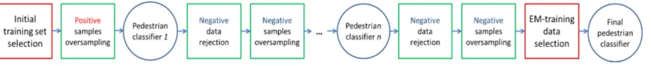
Figure 1: FairTrain training pipeline.

The training procedure that this paper advocates for unfolds as follows. After the initial data selection, we balance the negative and positive sample cardinalities. Then, a set of n negative data rejectors are trained and identified negative data are discarded. The validation set negative samples are iteratively oversampled after each training to ensure a balanced set. The final classifier is learned after careful data selection. Figure 1 illustrates the process. The next two sections respectively detail our data selection mechanism and our classifier training methodology.

4 Training Set Generation

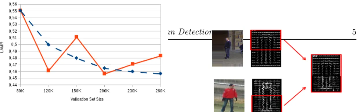
Let us run a simple experiment to illustrate our training set generation main idea. Figure 2 plots the performance on the INRIA dataset of a simple HoG classifier in relation to the validation set

(8)

Figure 2: Influence of the validation set size on a HoG clas-sifier (Experimentation on the INRIA dataset). Expected performance is in dashed blue, actual results in plain red. The used metric is the log-average miss rate (the lower the better).

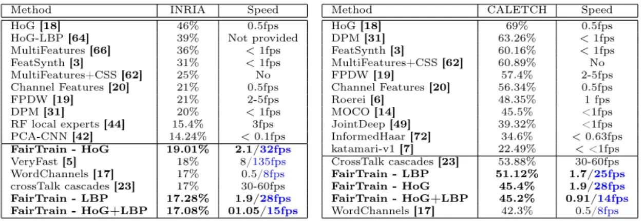
Figure 3: data generation example.

size. The training set (of size 10K) is determined using bootstrapping [18][30].

Performance should theoretically asymptotically increase with the validation set size. This assumption, depicted by the dashed curve on the Figure, corresponds to the common belief that the dataset informative power is directly correlated to its size. However, the results, plotted with the plain curve, are quite different from our expectations. They show significant irregularities as the dataset size increases; and the largest datasets do not even provide the best results. This encourages us to think twice about the way training data are considered: Apt data selection may be more important than their simple addition.

This is the principle underpinning our training set generation. The method is composed of several stages, detailed within the body of this section. We first select insightful positive and negative instances from the millions of extracted features. The minority class is then oversampled to create balanced training and validation sets. The third step generates an initial training set utilizing boostrapping [18][30]. Finally, we optimise this first set using an expectation-maximisation algorithm.

4.1 Instances selection

Ground truth positive examples are fed to the training set and near positives with a coverage higher than 90% to the validation set. For each image, data negative samples are sorted according to their similarity with positive examples and we then randomly select m instances among the most similar half (based on euclidean distance). A subset is added to the training set to match the positive sample cardinality and the rest is left to the validation set. This simple, yet efficient selection process focusses on hard data near the categories border. At this stage, we have constructed a tiny balanced training set and a large imbalanced validation set. The next steps oversample the validation set minority class and grows the training set.

4.2 Minority class oversampling

We augment the validation set in order for the two opposite classes to have the same cardinality. As the minority class is always the positive one, this comes down to augmenting the set of positive samples. For that purpose, we use a generative sampling algorithm that takes advantage of the possibility to geometrically locate the feature values within the bounding box. The method is then restricted to feature types that are geometrically structured, and have a precise location attached to their values, such as HoG [18], DPM [31], or Haar-inspired strategies [20].

The new data generation function f(.) unfolds as follows. We randomly select 2 instances x1= [x11, ...x1n]and x2= [x21, ...x2n]from the same class Si and create a new sample with their

lower and upper body features, while avoiding doublons. Uniform sampling with replacement is employed. More formally:

∀x1, x2∈ Si f (x1, x2) = [x11, ...x1n 2, x2

n

2+1, ...x2n] (1)

(9)

6 Remi Trichet, Francois Bremond So, a minority class of n samples can spawn a maximum of n × (n − 1) new instances. This process doesn’t suffer from the over-generalisation issue that mares other generative techniques, like SMOTE [63] as data pairs are not necessarily selected within the same neighborhood and the upper/lower body dichotomy rule guarantees a valid datum.

Of course, other geometrical dichotomies can be thought of as long as the final instance appearance, corresponding to the selected data feature combination, is credible. Moreover, vertical splits might be pointless, as lots of training data are often vertically mirrored during pre-processing. We do not normalise the final vector. In practice, this gives us slightly better results than a re-normalisation. The process is illustrated in the Figure 3.

4.3 Initial training set generation

We use bootstrapping [18][30] to augment the training set. At each iteration, we incorporate the most badly classified data from the validation set into the training set and retrain the classifier. We aim to repeat this process until the training set reaches its desired initial size T .

However, 2 iterations have been advised to avoid overfitting [62]. Therefore, we modified the algorithm to deal with this issue. Instead of simply selecting data from the validation set, we generate it the same way as detailed in the minority class oversampling section. Each new datum parent samples are selected among the misclassified data. Weighted sampling is utilised in this case, the probability of an instance to be drawn being set in relation to the extent of the error. We iterate until the desired training set size is reached or the validation set is perfectly classified.

4.4 Training set Optimisation

The proper selection of an apt training set is paramount for optimal classifier performance. Our purpose is to select the core training set data that will lead to improved classification. Our core idea is a typical machine learning one: Since we can hardly define what makes a good training set, we will let the algorithm learn it by itself. We utilise an expectation-maximisation algorithm for this purpose.

The algorithm unfolds as follows. Weights, initialised equal, are associated to the training data. At each iteration it, (M-step) we randomly select Dit/2positive and Dit/2negative data

from the training set to respect the class equality rule [70], the selection being guided by data weights. A new classifier Citis then trained on these Ditdata, and tested on the validation set.

(E-step) Weights are updated according to the classification performance. A sample’s weight is set according to the average classification performance over all the past runs for which it was selected. W (xi) =   X S_xi=[it|xi∈Dit] score(Cit)  /|Sxi| (2)

To further improve this algorithm, we set up a global confidence value for each validation datum. This value is the average confidence value for each datum over all the past iterations. Every m/10 iterations, this global confidence values are L1-normalised and utilised as probabil-ities to randomly generate new data based on the most badly classified data. In other words, we create additional data in areas of the feature space where extra information is required, like near the border between categories. This active learning mechanism improves the quality of the training set the same way bootstrapping [18][30] does. Consequently, the algorithm gives a better outcome when associated with a large validation set that will limit overfitting.

Dis set low at the beginning (i.e 5% of the training set) and progressively increased as the it-erations unfold until the desired training set size is reached. This allows the algorithm to focus on the core samples withholding the classifier first, before refining the set for optimal classification.

(10)

Also, running the bulk of the iterations with small training sets speeds up the algorithm and allows us to run the numerous iterations necessary for its reliability. The algorithm pseudo-code is :

Data:

A training set t of cardinality T , T weights associated to training data, a validation set v of cardinality V , V confidence values associated to validation data, V global confidence values as-sociated to validation data.

Result: Optimal training set o = O with O≤T Set weights to 1

Set globalConfs to 1 For(it=0; it<m; it++)

{

Bagging(weights, t, d); // Randomly select D/2 positive and D/2 negative data from the training set.

}

Cit= Train(d); // Train a classifier Citwith the D data.

Score = classify(Cit, v, confs); // Test the classifier on the validation set.

Update(weights, score); // Update weights.

Update(globalConfs, confs); // Update the global confidence values. If(Score > bestscore)

{

bestscore = Score; // Saving best training set. SaveClassifier()

}

If (it%(m/10) == 0) {

Generate(globalConfs, v, p); // Randomly generate P data among the most consistently badly classified.

t += p; // and add them to the training set }

Obviously, a large number of iteration is necessary for the algorithm to produce good results. For our experiments, we set m = 5000 when the algorithm is a standalone, and m = 1000 when it is used as the cascade-of-rejectors final classifier (see section 5). The training takes 16 hours to complete with 200K data using 12 cores; 6 hours for 10K data.

5 Cascade-of-Rejectors

The cascade-of-rejectors is an efficient strategy for sieving out a large proportion of false positives, and has been applied several times in the context of pedestrian detection [17][73] [8][58][61]. However, tuning this cascade of classifiers remains problematic. First, the classifiers are prone to errors that propagate along the cascade. Second, most authors employing this technique solely reject negative data after each classification step to avoid the creation of classifiers likely to reject positive data during the subsequent stages. However, this leads to progressively more imbalanced datasets. Fine tuning of the original positive versus negative instances ratio is usually necessary to obtain satisfactory results (a 2 to 4 times bigger negative set is the common practice). But this strategy is still under-optimal as balanced datasets are proved [70] to be the best performing ones.

To deal with these issues, we propose a new cascade-of-rejectors. Our approach borrows [39]’s main idea with a two-stage classification: The first one aims for a high recall whereas the second one focuses on precision.

(11)

8 Remi Trichet, Francois Bremond The first stage embodies a cascade of n − 1 rejectors. To avoid increasing the false negative rate, these n − 1 initial classifiers enforce a high recall, moderately optimizing the performance on the precision. The metric formalises as:

M = (T N × WT N+ T P )/(P + N ) (3)

with P, N, T P, T N, and WT N being respectively positive, negative, true positive, true negative

instances, and the weight associated to T N. WT N is set at WT N = 0.5. Its parametrisation

has no influence on the results, when set low enough, which enforces a perfect or near perfect recall. Negative data, with a confidence below 0.5, are rejected at each stage. Negative data over-sampling is then undertaken to avoid emptying the validation set. When insufficient to match the positive instances cardinality, random positive data under-sampling is then considered. We employ Adaboost as classifiers for this part. These decision trees have demonstrated competitive performance whilst retaining computational efficiency [67][45]. During testing, typically over 95% of the data are safely discarded after 4-5 iterations. This cascade-of-rejectors guaranties a high recall, increased performance induced by balancing the datasets at each iteration, and few parameters to tune.

The second stage performs a finer classification, aiming for high precision results. Since the bulk of the data have been removed, more demanding computation can be performed at this stage without slowing down the detector. We employ a dense forest classifier, that has shown [7] giving slightly better performance than its counterparts on pedestrian detection. We optimise for the log-average miss rate [51].

The only parameter that requires careful tuning is the rejection threshold T value during the testing phase. Since the method optimises for the recall, the large majority of data around the separating border between the two classes are negative ones. It is then sensible to set T > 0.5. The two employed classifiers in this work are typical Adaboost [68] and random forest [11]. See the experiment section for a thorough evaluation of this parameter impact on performance.

6 Experiments

This section, dedicated to our experimental validation, breaks down into three sub-parts: exper-imental setup details, results and related comments, and finally parameter discussion.

6.1 Experimental setup

We experimented on the INRIA [18] and Caltech-USA (reasonnable set) [25] datasets with HoG [18]and Haar-LBP [16] features. HoGs are configurated with 12 × 6 cells, 2 × 2 blocks and 12 angle orientations, for a total of 2640 values. Block as well as full histogram normalisation are performed. The LBP descriptor follows the same structure, features a value per channel for each cell, and non-uniform patterns are pruned out [47]. Candidates are selected using a multi-scale sliding window approach [73] with a stride of 4 pixels. Approximately 60% are loosely filtered according to "edgeness" and symmetry. No background subtraction or motion features are em-ployed on the Caltech dataset. The training set size is up-bounded at 12K samples. Increasing this threshold doesn’t improve performance.

We also clean the data based on Tomek links [60]. We employ euclidian distance and restrict the deletion to negative data to spare the scarce minority class. Approximately 0.1% to 0.2% of the negative data are removed this way. No generative resampling is performed. The model height is set to 100 pixels for the INRIA dataset, 50 pixels for Caltech.

We also implemented a cascade-of-rejectors baseline with the commonly used settings: Re-jector optimisation is done according to the log-average miss rate metric. We tested this baseline with a typical initial validation set containing 4 times more negative samples than positive ones. To compare with the common multi-dataset training technique, we also used an augmented ver-sion with PETS2009 [32] positive samples. This set gathers 50K positive instances from both

(12)

datasets and 110K negatives from the sole INRIA benchmark.

We utilised the openCV implementation for the Adaboost and random forest classifiers. Ran-dom forest parameter set includes the number of decision trees, the number of sampled feature dimensions and the max tree depth. They were selected by measuring out-of-bag errors (OOB) [11]. It was computed as the average of prediction errors for each decision tree, using the non-selected training data. Adaboost is initialised with a tree depth of 2 and 256 weak classifiers. Each extra run adds 64 weak classifiers. This is a low number of weak classifiers compared to typical settings (i.e. [1024, 2048]). However, in practice, increasing this value leads us to lower performance and speed.

We use a variant of the threshold non-maximum suppression (t-NMS) [13] that groups the detections according to the bounding boxes overlap with the group d best candidate, keeps the d candidates with highest confidence for each group, and builds the final candidate position with the group mean border positions. We set the overlap threshold to 0.6 and d = 3 for all our experiments. Log-Average Miss Rate (LAMR) [51] is employed as metric for all runs.

6.2 Results

Run Validation Set Size #Rejectors Final Classifier Optimization LAMR Performance

1 180K (INRIA) 0 A n.a. 46.03%

2 180K (INRIA) 5 A n.a. 43.38%

3 160K (INRIA+PETS) 5 A n.a. 42.44%

4 180K (INRIA) 0 EM training(A) n.a. 39.72%

5 180K (INRIA) 0 EM training(RF) n.a. 40.34%

6 180K (INRIA) 5 A LAMR/Recall 21.64% / 21.09%

7 180K (INRIA) 5 RF LAMR/Recall 21.34% / 20.98%

8 180K (INRIA) 5 EM training(RF) LAMR/Recall 20.39% / 20.15% 9 220K (INRIA) 5 EM training(RF) LAMR/Recall 20.25% / 19.68% 10 250K (INRIA) 5 EM training(RF) LAMR/Recall 20.54% / 19.67% 11 300K (INRIA) 5 EM training(RF) LAMR/Recall 19.52% / 19.01% 12 220K (INRIA) 6 EM training(RF) LAMR/Recall 19.82% / 19.38%

Table 1: Log-average miss rate results (the lower the better) of FairTrain with various components and settings on the INRIA dataset with HoG features. Baselines are in bold. A - Adaboost. RF - Random Forest. EM - Expectation-Maximisation. LAMR - Log-average miss rate. Baselines are in bold.

Method INRIA Speed

HoG [18] 46% 0.5fps

HoG-LBP [64] 39% Not provided MultiFeatures [66] 36% < 1fps FeatSynth [3] 31% < 1fps MultiFeatures+CSS [62] 25% No Channel Features [20] 21% 0.5fps FPDW [19] 21% 2-5fps DPM [31] 20% < 1fps RF local experts [44] 15.4% 3fps PCA-CNN [42] 14.24% < 0.1fps FairTrain - HoG 19.01% 2.1/32fps VeryFast [5] 18% 8/135fps WordChannels [17] 17% 0.5/8fps crossTalk cascades [23] 17% 30-60fps FairTrain - LBP 17.28% 1.9/28fps FairTrain - HoG+LBP 17.08% 01.05/15fps

Method CALETCH Speed

HoG [18] 69% 0.5fps DPM [31] 63.26% < 1fps FeatSynth [3] 60.16% < 1fps MultiFeatures+CSS [62] 60.89% No FPDW [19] 57.4% 2-5fps Channel Features [20] 56.34% 0.5fps Roerei [6] 48.35% 1 fps MOCO [14] 45.5% <1fps JointDeep [49] 39.32% <1fps InformedHaar [72] 34.6% < 0.63fps katamari-v1 [7] 22.49% < <1fps CrossTalk cascades [23] 53.88% 30-60fps FairTrain - LBP 51.12% 1.7/25fps FairTrain - HoG 45.4% 1.9/28fps FairTrain - HoG+LBP 45.2% 0.91/14fps WordChannels [17] 42.3% 0.5/8fps

Table 2: Comparison with the state-of-the-art. Near real-time methods are separated from others. FairTrain is in bold. Computation times are calculated according to 640×480 resolution frames. The used metric is the log-average miss rate (the lower the better). The speed(CPU/GPU) is in frame per seconds (fps)

Detailed method results on the INRIA dataset, including the influence of its various com-ponents and settings are reported in Table 1. The expectation-maximisation (EM) training leads to an average 6% improvement over simple HoG-based classification, or 2.3% over the common cascade-of-rejectors. This demonstrates the importance of proper data selection. The

(13)

10 Remi Trichet, Francois Bremond

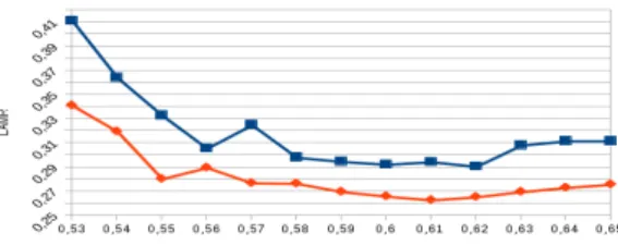
Figure 4: Influence of the rejection threshold T on per-formance. The blue and red curves respectively depict ver-sions with Adaboost and an EM trained random forest as final classifiers. Log-average miss rate is used as metric (the lower the better) and rejector optimisation function.

main boost is obtained by our modified version of the cascade-of-rejectors, with a minimum 24% performance increment. Finally, the combined algorithms lead to a further 3% improvement. To sum up, FairTrain gives a simple HoG based detector an impressive 27% boost, therefore competing with state-of-the-art real-time references. It significantly outperforms the usual blend of datasets strategy (see Table 1 - run 3), scoring only 42.44%.

The main factor responsible for the cascade-of-rejectors significant results is the balanced generative dataset. max-recall optimisation also has a slight, but steady influence on perfor-mance, with an average 0.51% better score. Similarly, we found random forest to outperform Adaboost as final classifier by approximately 0.4% on all EM runs. Finally, in accordance with the literature [17][73][8], we observed that optimal results are obtained for 5 iterations of the rejection cascade, the addition of extra iterations being impactless, as shown in Table 1 - run 12. We have tested this algorithm for various validation set sizes (see Table 1 - runs 8 to 11) to replicate the section 4 theoretical experiment (see Figure 2). Results show much more stable performance, therefore validating our primary assumption as well as the approach stemming from it.

Table 2 shows our method’s ranking compared to the state-of-the-art, in terms of performance and speed. T =0.58 is used for these runs. This work compares favorably to the state-of-the-art. While not being the best detector on the market, with respectively 17% and 47% log-average miss rate on the INRIA and Caltech datasets, FairTrain still provides a very competitive per-formance/speed ratio. For instance, it scores better than the famous DPM [31] and similarly to the integral channel features [19] while running 4 times faster. VeryFast [5] and the crosstalk cascades provide a viable alternative in terms of speed while displaying lower performance. LBP is the best descriptor on the INRIA dataset, while HoGs show the best performance on Cal-tech. We assume that the numerous little pedestrians on the latter impact the texture descriptor more strongly than the gradients. The HoG and LBP fusion yields little improvement. Packed crowds, teensy pedestrians and awkward poses remain the main failure cases. For a near optimal parametrisation of T , pruning out approximately 70% of the data during the first iteration, the succession of classifiers overall multiplies by 1.4 the computation load. The end-to-end system processes 2 fps on an Intel Xeon 2.1GHz CPU, calculated over frames of 640×480 pixels in size. Further speed up is possible when using a GPU, leading our detector to perform in real-time. This makes FairTrain one of the best performing real-time pedestrian detector to date.

6.3 Parameter Sensitivity

The rejection threshold T from the cascade-of-rejectors has a critical influence on both, results and computation time. Indeed, the more data are removed at each classification step, the faster the detector will be. Also, since there is a high imbalance of positive/negative instances during testing, it is sensible to yield better results for T > 0.5. Moreover, optimizing rejection cascade classifiers for a high recall further accentuates this bias. Figure 4 plots its influence on the results when optimizing for log-average miss rate with two different final classifiers: Adaboost and EM-optimised random forest. We observe that the results are more stable across the parameter range when the expectation-maximisation optimisation of the training set is employed. This further validates the use of this algorithm. The optimal testing confidence threshold is within the range

(14)

[0.58, 0.6]for all tests whether we are optimizing for log-average miss rate or to the recall. For all runs, a low standard deviation is observed within this optimal range (typically, .5%). This demonstrates the stability of this parameter. We explain the similar parameter setting (and performance) of the two optimisation techniques with their overall similarity. Indeed, log-average miss rate also intrinsically optimises for recall. Even though it provides lower performance in our case, an automatic threshold estimation of T for each separate classifier may theoretically lead to further improvement.

7 Conclusion

This paper explored data selection mechanisms for near real-time pedestrian detection. Via Fair-Train, we introduced an expectation-maximisation data weighting scheme for enhanced training set generation. We also improved the cascade-of-rejectors by enforcing balanced datasets at every step of the classification and separately optimizing for recall and precision. The method showed competitive results compared to the state-of-the art and major performance boost when compared to original features.

By proving that blind data addition is not the best way to enhance a training set, this work brings up an important question: Then, what makes a good training set ? Or even a good training datum ? Future experimentation will be an attempt of response. Also, the addition of more recent features and further work on classifier combination is envisioned.

References

[1] A. Alahi, L. Jacques, Y. Boursier, , and P. Vandergheynst. Sparsity-driven people localiza-tion algorithm: Evalualocaliza-tion in crowded scenes environments. PETS workshop, 2009. [2] D. Arsic, A. Lyutskanov, G. Rigoll, and B. Kwolek. Multi-camera person tracking applying

a graph-cuts based foreground segmentation in a homography framework. PETS workshop, 2009.

[3] A. Bar-Hillel, D. Levi, E. Krupka, and C. Goldberg. Part-based feature synthesis for human detection. ECCV, 2010.

[4] R. Benenson, M. Mathias, R. Timofte, and L. Van Gool. Pedestrian detection at 100 frames per second. CVPR, 2012.

[5] R. Benenson, M. Mathias, R. Timofte, and L. Van Gool. Pedestrian detection at 100 frames per second. CVPR, 2013.

[6] R. Benenson, M. Mathias, T. Tuytelaars, and L. Van Gool. Seeking the strongest rigid detector. CVPR, 2013.

[7] R. Benenson, M. Omran, J. Hosang, and B. Schiele. Ten years of pedestrian detection, what have we learned? ECCV, CVRSUAD workshop, 2014.

[8] B. Berkin, B. K.P. Horn, and I. Masaki. Fast human detection with cascaded ensembles on the gpu. IEEE Intelligent Vehicles Symposium, 2010.

[9] M. Bertozzi, A. Broggi, P. Grisleri, T. Graf, and M. Meinecke. Pedestrian detection in infrared images. IEEE Intelligent Vehicles Symp., 2003.

[10] L. Bourdev and J. Malik. Poselets: Body part detectors trained using 3d human pose annotations. ICCV, 2009.

(15)

12 Remi Trichet, Francois Bremond [11] L. Breiman. Random forests. Machine Learning, 2001.

[12] M. D. Breitenstein, F. Reichlin, B. Leibe, E. Koller-Meier, and L. van Gool. Markovian tracking-by-detection from a single, uncalibrated camera. PETS workshop, pages 71–78, 2009.

[13] M. Diez Buil. Non-maximum suppression. technical report ICG-TR-xxx, 2011.

[14] G. Chen, Y. Ding, J. Xiao, and T. X. Han. Detection evolution with multi-order contextual co-occurrence. CVPR, 2013.

[15] D. Conte, P. Foggia, G. Percannella, and M. Vento. Performance evaluation of a people tracking system on the pets video database. PETS workshop, 2009.

[16] E. Corvee and F. Bremond. Haar like and lbp based features for face, head and people detection in video sequences. ICVS, 2011.

[17] A. D. Costea and S. Nedevschi. Word channel based multiscale pedestrian detection without image resizing and using only one classifier. CVPR, 2014.

[18] N. Dalal and B. Triggs. Histograms of oriented gradients for human detection. CVPR, 2005. [19] P. Dollar, S. Belongie, and P. Perona. The fastest pedestrian detector in the west. BMVC,

2010.

[20] P. Dollar, Z. Tu, P. Perona, and S. Belongie. Integral channel features. BMVC, 2009. [21] P. Dollar, C. Wojek, B. Schiele, and P. Perona. Pedestrian detection: A benchmark. CVPR,

2009.

[22] P. Dollar, C. Wojek, B. Schiele, and P. Perona. Pedestrian detection: An evaluation of the state of the art. PAMI, 2012.

[23] P. DollÃ¡r, R. Appel, and W. Kienzle. Crosstalk cascades for frame-rate pedestrian detec-tion. ECCV, 2012.

[24] P. DollÃ¡r, S. Belongie, and P. Perona. The fastest pedestrian detector in the west. BMVC, 2010.

[25] P. DollÃ¡r, C. Wojek, B. Schiele, and P. Perona. Pedestrian detection: A benchmark. CVPR, 2009.

[26] C. Elkan. The foundations of cost-sensitive learning. Intl Joint Conf. Artificial Intelligence, 2001.

[27] A. Ellis and J. Ferryman. Pets2010 and pets2009 evaluation of results using individual ground truthed single views. AVSS, 2010.

[28] Y. Fang, K. Yamada, Y. Ninomiya, and I. Masaki. Comparison between infrared-image-based and visible- image-infrared-image-based approaches for pedestrian detection. IEEE Intelligent Vehi-cles Symp., 2003.

[29] P. Felzenszwalb, D. McAllester, and D. Ramanan. A discriminatively trained, multiscale, deformable part model. CVPR, 2008.

(16)

[30] P. F. Felzenszwalb, R. B. Girshick, and D. McAllester. Cascade object detection with deformable part models. CVPR, 2010.

[31] P.F. Felzenszwalb, R.B. Girshick, D. McAllester, and D. Ramanan. Object detection with discriminatively trained part-based models. PAMI, 32(9):1627–1645, 2009.

[32] J. Ferryman and A. Shahrokni. An overview of the pets2009 challenge. PETS, 2009. [33] J. Gall and V. Lempitsky. Class-specific hough forests for object detection. CVPR, 2009. [34] C. Galleguillos and S. Belongie. Context based object categorization: A critical survey.

CVIU, 114:712–722, 2010.

[35] H. Han, W.Y. Wang, and B.H. Mao. Borderline-smote: A new over-sampling method in imbalanced data sets learning. Intl Conf. Intelligent Computing, 2005.

[36] H. He, Y. Bai, E.A. Garcia, and S. Li. Adasyn: Adaptive synthetic sampling approach for imbalanced learning. Intl J. Conf. Neural Networks, 2008.

[37] H. He and E. A. Garcia. Learning from imbalanced data. IEEE transactions on Knowledge and data engineering, 21(9), 2009.

[38] A. Hoiem and M.H. Efros. Putting objects in perspective. IJVC, 2008.

[39] S. Hwang, T.-H. Oh, and I. S. Kweon. A two phase approach for pedestrian detection. ACCV, 2014.

[40] N. Japkowicz. Learning from imbalanced data sets: a comparison of various strategies. AAAI Workshop on Learning from Imbalanced Data Sets, 2000.

[41] T. Jo and N. Japkowicz. Class imbalances versus small disjuncts. ACM SIGKDD Explo-rations Newsletter, 6(1):40–49, 2004.

[42] W. Ke, Y. Zhang, P. Wei, Q. Ye, and J. Jiao. Pedestrian detection via pca filters based convolutional channel features. ICASSP, 2015.

[43] H. Kiani. Multi-channel correlation filters for human action recognition. ICIP, 2014. [44] J. Marin, David Vazquez, A. M. Lopez, J. Amores, and B. Leibe. Random forests of local

experts for pedestrian detection. ICCV, 2013.

[45] W. Nam, P. Dollar, and J. H. Han. Local decorrelation for improved pedestrian detection. NIPS, 2014.

[46] W. Nam, P. Dollar, and J. H. Han. Local decorrelation for improved pedestrian detection. NIPS, 2014.

[47] T. Ojala, M.PietikÃ¤inen, and T. MÃ¤enpÃ¤Ã¤. Multiresolution gray-scale and rotation invariant texture classification with local binary patterns. PAMI, 2002.

[48] W. Ouyang and X. Wang. Joint deep learning for pedestrian detection. ICCV, 2013. [49] W. Ouyang and X. Wang. Joint deep learning for pedestrian detection. ICCV, 2013. [50] W. Ouyang and X. Wang. Single-pedestrian detection aided by multi-pedestrian detection.

CVPR, 2013.

(17)

14 Remi Trichet, Francois Bremond [51] Dollar P, C. Wojek, B. Schiele, and P. Perona. Pedestrian detection: An evaluation of the

state of the art. PAMI, 34:743–761, 2012.

[52] M. Jones P. Viola. Robust real-time face detection. IJCV, 2004.

[53] D. Park, D. Ramanan, and C. Fowlkes. Multiresolution models for object detection. ECCV, 2010.

[54] D. Park, C.L. Zitnick, D. Ramanan, and P. DollÃ¡r. Exploring weak stabilization for motion feature extraction. CVPR, 2013.

[55] J. Prokaj and G. Medioni. Persistent tracking for wide area aerial surveillance. CVPR, 2014.

[56] M. Ristin, J. Gall, and L. Van Gool. Local context priors for object proposal generation. ACCV, 2012.

[57] W. Schwartz, L.S. Davis, and H. Pedrini. Local response context applied to pedestrian detection. CIARP, 2011.

[58] M. Souded and F. Bremond. Optimized cascade of classifiers for people detection using covariance features. VISAPP, 2013.

[59] K.M. Ting. An instance-weighting method to induce cost-sensitive trees,. IEEE Trans. Knowledge and Data Eng., 14(3):659–665, 2002.

[60] I. Tomek. Two modifications of cnn. IEEE Trans. System, Man, Cybernetics, 6(11):769–772, 1976.

[61] Viola and M. Jones. Rapid object detection using a boosted cascade of simple features. CVPR, 2001.

[62] S. Walk, N. Majer, K. Schindler, and B. Schiele. New features and insights for pedestrian detection. CVPR, 2010.

[63] B.X. Wang and N. Japkowicz. Imbalanced data set learning with synthetic samples. IRIS Machine Learning Workshop, 2004.

[64] X. Wang, T. X. Han, and S. Yan. An hog-lbp human detector with partial occlusion handling. ICCV, 2009.

[65] O. Williams, A. Blake, and R. Cipolla. A sparse probabilistic learning algorithm for real-time tracking. ICCV, 2003.

[66] C. Wojek and B. Schiele. A performance evaluation of single and multi-feature people detection. DAGM Symposium Pattern Recognition, 2008.

[67] B. Wu and R. Nevatia. Cluster boosted tree classifier for multi-view, multi-pose object detection. ICCV, 2007.

[68] R. Shapire Y. Freund. A decision-theoric generalization of online learning and an application to boosting. Journal of Computer and System Sciences, 1997.

[69] J. Yan. Robust multi-resolution pedestrian detection in traffic scenes. CVPR, 2013.

(18)

[70] R. Yan, Y. Liu, R. Jin, and A. G. Hauptmann. On predicting rare classes with svm ensemble in scene classification. ICASSP, 2003.

[71] J. Yang, Z. Shi, P. Vela, and J. Teizer. Probabilistic multiple people tracking through complex situations. PETS workshop, 2009.

[72] S. Zhang, C. Bauckhage, and A. B. Cremers. Informed haar-like features improve pedestrian detection. CVPR, 2014.

[73] Q. Zhu, S. Avidan, M. Yeh, and K. Cheng. Fast human detection using a cascade of histograms of oriented gradients. CVPR, 2006.

(19)

RESEARCH CENTRE

SOPHIA ANTIPOLIS – MÉDITERRANÉE 2004 route des Lucioles - BP 93 06902 Sophia Antipolis Cedex

Publisher Inria

Domaine de Voluceau - Rocquencourt BP 105 - 78153 Le Chesnay Cedex inria.fr