http://dx.doi.org/ 10.3168/jds.2011-4322
© American Dairy Science Association®, 2012 .
ABSTRACT
The aim of this research was to compare different Bayesian procedures to integrate information from out-side a given evaluation system, hereafter called external information, and in this context estimated breeding values (EBV), into this genetic evaluation, hereafter called internal evaluation, and to improve the Bayesian procedures to assess their potential to combine infor-mation from diverse sources. The 2 improvements were based on approximations of prior mean and variance. The first version of modified Bayesian evaluation con-siders all animals as animals associated with external information. For animals that have no external infor-mation (i.e., internal animals), external inforinfor-mation is predicted from available external information. Thereby, propagation of this external information through the whole pedigree is allowed. Furthermore, the prediction of external information for internal animals allows large simplifications of the computational burden during setup and solving of mixed model equations. However, double counting among external animals (i.e., animals associated with available external information) is not avoided. Double counting concerns multiple consider-ations of contributions due to relconsider-ationships by integra-tion of external EBV for related external animals and is taken into account by the second version of modified Bayesian evaluation. This version includes the estima-tion of double counting before integraestima-tion of external information. To test the improvements, 2 dairy cattle populations were simulated across 5 generations. Milk production for the first lactation for each female was simulated in both populations. Internal females were randomly mated with internal males and 50 external males. Results for 100 replicates showed that rank cor-relations among Bayesian EBV and EBV based on the joint use of external and internal data were very close to 1 for both external and internal animals if all inter-nal and exterinter-nal animals were associated with exterinter-nal information. The respective correlations for the internal
evaluation were equal to 0.54 and 0.95 if no external information was integrated. If double counting was avoided, mean squared error, expressed as a percentage of the internal mean squared error, was close to zero for both external and internal animals. However, compu-tational demands increased when double counting was avoided. Finally, the improved Bayesian procedures have the potential to be applied for integrating external EBV, or even genomic breeding values following some additional assumptions, into routine genetic evalua-tions to evaluate animals more reliably.
Key words: Bayesian approach , dairy cow , integra-tion , external informaintegra-tion
INTRODUCTION
Theoretical properties of currently used methods to assess the genetic value of domestic animals depend on certain conditions. One of the most important is that all available information has to be used simultaneously to obtain unbiased estimates (e.g., Henderson, 1984). However, this is often not the case in practice, for many potential reasons. The most important issue is the un-availability of raw data (e.g., recorded and evaluated in another country) or the complexity of computations that require the use of multi-step, sequential, or dis-tributed computing. Both issues are frequent in modern breeding, especially in dairy cattle breeding, because international exchange of genetic material (e.g., frozen semen and embryos) is extremely widespread. Until now, basic genetic evaluations are mostly based on local data, potentially followed by an international second step, as performed by the International Bull Service (Interbull, Uppsala, Sweden) for dairy breed sires. However, the accuracy of local evaluations may be limited for animals with few local data. Furthermore, the current massive development of genomic selection exacerbates this issue, because potentially more dif-ferent genetic evaluations may exist, and the need to combine those sources of information increases. Cur-rent methods used in the context of dairy cattle are mostly selection index based on VanRaden (2001) to combine different sources of information (e.g., Gengler and VanRaden, 2008).
Comparison and improvements of different Bayesian procedures
to integrate external information into genetic evaluations
J. Vandenplas *†1 and N. Gengler *†
* Animal Science Unit, Gembloux Agro Bio-Tech, University of Liège, B-5030 Gembloux, Belgium † National Fund for Scientific Research, B-1000 Brussels, Belgium
Received February 28, 2011. Accepted October 17, 2011.
1514 VANDENPLAS AND GENGLER
Journal of Dairy Science Vol. 95 No. 3, 2012
Another promising class of methods is based on Bayesian methods originating from the work from Klei et al. (1996) in the context of multibreed genetic evaluations for beef cattle. In this context, Bayesian means that the prior distribution of breeding values is changed according to what is known from an external source. Later, Quaas and Zhang (2001) and Legarra et al. (2007) proposed 2 different Bayesian derivations to incorporate external information, including external genetic breeding evaluations and their associated ac-curacies, into the internal evaluation. The integration of external information leads to an improved ranking of animals with external information (so-called exter-nal animals) in the interexter-nal evaluation, which is more similar to the ranking of a hypothetical joint evaluation of internal and external animals. Another advantage of this integration is that accuracies of EBV for external animals are more reliable compared with those of the internal evaluation. Furthermore, this improvement of accuracies and rank correlations of external animals between the internal and joint evaluations depends on the external accuracy of prior information (Quaas and Zhang, 2001, 2006; Zhang et al., 2002; Legarra et al., 2007) but also on several hypotheses used in the imple-mentation. For example, current implementations do not take into account the double counting among exter-nal animals. However, an EBV of an animal combines information from its own records and from records of all relatives through its parents and its offspring (Misztal and Wiggans, 1988; VanRaden, 2001). Integrated exter-nal information of this animal and a close relative into the same genetic evaluation may be counted double if this external information contains both contributions due to relationships. Furthermore, until now, only few proposals exist to put these methods in the context of dairy cattle breeding, whereas they can be used in many situations and as a way to integrate genomic pre-diction (e.g., Gengler and Verkenne, 2007).
The first aim of this research was to compare dif-ferent Bayesian approaches for their potential to com-bine information from diverse sources and the second aim was to improve existing Bayesian approaches to integrate external information into genetic evaluations. Focus was thereby given to the simplification of the computational burden and the avoidance of double counting among external animals.
MATERIALS AND METHODS
Theoretical Background
Different concepts that will be used in this study are defined as follows: (1) Internal data was defined as data used only for internal evaluations (e.g., milk records in a given country A). (2) External data was defined as
additional data not directly used in internal evaluations (e.g., milk records in another given country B). (3) In-ternal information was related to information obtained from an evaluation based only on internal data (e.g., local EBV in country A). (4) External information was related to information obtained from an evaluation based only on external data and free of internal infor-mation (e.g., foreign EBV or genomic EBV obtained in country B). Finally, all animals were distinguished between internal and external animals. (5) An internal animal was an animal associated with only internal data and internal information (e.g., locally used sires in country A). (6) An external animal was an animal associated with external data and information and also having internal data and information or being relative to the evaluation of internal animals (e.g., foreign sires also used in country A in addition to country B or genotyped animals from country B relevant to country A).
The main reason for the application of Bayesian procedures is to obtain solutions as close as possible to those of a hypothetical joint evaluation of all exter-nal and interexter-nal animals including their data. This is performed by integrating external information into the internal genetic evaluation instead of using only inter-nal data. The considered exterinter-nal information in this context was available external EBV and their associ-ated accuracies obtained from only external data (yE). Both will be used to define the prior distribution of the internal EBV of the external animals (uE). This prior distribution can be defined in a generic way as p(uE|yE) = MVN(μ0 – Ub,G*), where MVN is multivariate
nor-mal, μ0 is the vector of external EBV of a joint genetic
evaluation of all internal and external animals based only on external data yE, G* is the matrix of predic-tion error (co)variances of these EBV, b is a vector of base differences between external and internal EBV, and U is an incidence matrix relating base differences to animals.
If E and I refer to external and internal evaluations,
respectively, and based on Legarra et al. (2007), a generic model can be written leading to these mixed model equations [1], representing this multi-trait modi-fied mixed model:
X R X X R Z 0 Z R X Z R Z G G U 0 U G U G I I1 I I I1 I I I1 I I I1 I * 1 * 1 * 1 * ′ ′ ′ ′ ′ ′ − − − − − − − + − − − − ⎡ ⎣ ⎢ ⎢ ⎢ ⎢ ⎢ ⎢ ⎤ ⎦ ⎥ ⎥ ⎥ ⎥ ⎥ ⎥ ⎡ ⎣ ⎢ ⎢ ⎢ ⎢ ⎢ ⎤ ⎦ ⎥ ⎥ ⎥ ⎥ ⎥ = 1 I I I1 I I I1 U u b X R y Z R ˆ ˆ ˆ β ′ ′ yy G U G I * 1 0 * 1 0 + ⎡ ⎣ ⎢ ⎢ ⎢ ⎢ ⎢ ⎢ ⎤ ⎦ ⎥ ⎥ ⎥ ⎥ ⎥ ⎥ − − μ μ ′ , [1]
where yI is the vector of internal observations, βI is the vector of fixed effects, u is the vector of random genetic effects of the external and internal random genetic ef-fects, XI and ZI are the incidence matrices for internal fixed effects and animals, respectively, and RI is the (co)variance matrix for the internal residual effects. Legarra et al. (2007) showed that:
G G G G G * 1 EE EI IE II − =⎡ + ⎣ ⎢ ⎢ ⎢ ⎤ ⎦ ⎥ ⎥ ⎥ Λ , where Λ is equal to Λ =D−1−G− EE1, [2]
where the matrix D is the matrix of prediction error (co)variances of the external information estimated from a genetic evaluation of all external animals based only on external data which did not include relation-ships between the internal animals, and G−EE1 is the in-verse of the additive genetic (co)variance matrix that only accounts for the relationships among external ani-mals. It is important to note that the matrix G−EE1 is different from GEE, because the latter also includes contributions from internal progeny of external ani-mals. Differences between G−EE1 and GEE can be illus-trated by writing the inverse of G in block form:
G G G G G G G G G G G 1 EE EI IE II 1 EE EI IE II EE 1 E − − − = = = + ⎡ ⎣ ⎢ ⎢ ⎤ ⎦ ⎥ ⎥ ⎡ ⎣ ⎢ ⎢ ⎢ ⎤ ⎦ ⎥ ⎥ ⎥ E E 1 EI II IE EE 1 EE 1 EI II II IE EE 1 II IE EE 1 EI G G G G G G G G G G (G G G G − − − − − − − − ))−1 ⎡ ⎣ ⎢ ⎢ ⎢ ⎤ ⎦ ⎥ ⎥ ⎥, where G−1 is the inverse of the additive genetic (co) variance matrix G that accounts for all the relation-ships among all external and internal animals.
It has also been shown that
D−1 =Z R Z′E E−1 E+G−EE1, [3] and that G D 0 * 1 0 1 E − =⎡ − ⎣ ⎢ ⎢⎢ ⎤ ⎦ ⎥ ⎥⎥ μ μ , [4]
where μE is a vector of external EBV from a genetic evaluation of all external animals based only on
exter-nal data that did not include relationships between the internal animals (Legarra et al., 2007).
Four Different Implementations
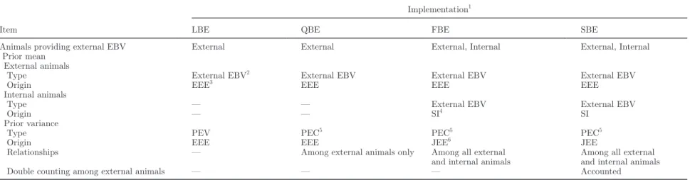
To be used, the generic system of equations [1] often needs to be simplified. In fact, usually only functions of external prediction error variances (PEV; e.g., reli-abilities), are available for approximating D and G*. Furthermore, μ0 is an unknown vector that needs to be estimated for some implementations. In this study, 4 different Bayesian implementations using gradually better approximations of prior mean and prior variance are compared (Table 1). The differences were related to the animals providing external information and to the way that the prior mean and variance were defined. The first implementation, hereafter called Legarra-type Bayesian evaluation (LBE), was the simplest one from a computational standpoint, as only external PEV were considered to approximate D. The second implementation, hereafter called Quaas-type Bayesian evaluation (QBE), included covariances among traits. Both implementations defined prior means based on external EBV obtained from the genetic evaluation of all external animals based only on external data, which did not include relationships among internal animals. The QBE can be computationally simplified as shown in the third implementation, hereafter called first ver-sion of modified Bayesian evaluation (FBE). Finally, the last implementation, hereafter called second version of modified Bayesian evaluation (SBE), approximated and used the across-animal covariances that are not reported in practice while existing in D.
LBE. Legarra et al. (2007) proposed a Bayesian
im-plementation to integrate prior information into an in-ternal genetic evaluation. The prior mean of the imple-mentation was defined as μE − UEbE, where μE = E(uE|yE), UE is an incidence matrix relating base dif-ferences to external animals, and bE is a vector of base differences among external and internal EBV for all the external animals. The prior variance D was approxi-mated by a diagonal matrix in which diagonal elements were equal to PEV associated to every external evalua-tion. Furthermore, this approximation of D implied another approximation to estimate Λ. Because
Λ =D−1−G−
EE1, all relationships needed to be ignored, and only diagonal elements of the matrix GEE were used. If nondiagonal elements in GEE were taken into account, the matrix G* could be non-semi-positive definite (Legarra et al., 2007; Gengler and Vanderick, 2008).
From a computational standpoint, the LBE method is rather simple to set up as the matrix D is considered diagonal. Gengler and Vanderick (2008) reported that
1516
V
ANDENPLAS AND
GENGLER
Journal of Dairy Science V
ol. 95 No. 3, 2012
Table 1. Main differences concerning the prior mean and variance among Legarra-type Bayesian evaluation, Quaas-type Bayesian evaluation, first version of modified Bayesian
evaluation, and second version of modified Bayesian evaluation
Item
Implementation1
LBE QBE FBE SBE
Animals providing external EBV External External External, Internal External, Internal
Prior mean External animals
Type External EBV2 External EBV External EBV External EBV
Origin EEE3 EEE EEE EEE
Internal animals
Type — — External EBV External EBV
Origin — — SI4 SI
Prior variance
Type PEV PEC5 PEC5 PEC5
Origin EEE EEE JEE6 JEE
Relationships — Among external animals only Among all external
and internal animals
Among all external and internal animals
Double counting among external animals — — — Accounted
1
LBE = Bayesian evaluation following Legarra et al. (2007) and using external EBV and prediction error variances (PEV) associated with external sires obtained from the external evaluation. QBE = Bayesian evaluation following Quaas and Zhang (2006) and using external EBV and PEV associated with external sires obtained from the external evaluation. FBE = Bayesian evaluation using external EBV and PEV associated with external sires obtained from the external evaluation where external EBV for all internal and external animals were predicted and used. SBE = Bayesian evaluation using external EBV and PEV associated with external sires obtained from the external evaluation where external EBV for all internal and external animals were predicted and used and the double counting among external animals was avoided.
2External EBV = EBV adjusted for base differences among external and internal information.
3
EEE = genetic evaluation of all external animals based only on external data that did not include relationships among the internal animals.
4SI = selection index.
5
PEC = prediction error covariances among traits (for FBE) and among traits and animals (for SBE).
LBE could be easily integrated into a test-day model for dairy cattle genetic evaluations with few modi-fications of the code of the used programs and with reasonable convergence. However, the method needs to compute the base differences among external and inter-nal information, which was estimated by Gengler and Vanderick (2008) before using the external information. This strategy avoids the computationally expensive in-tegrated estimation of base differences.
QBE. Quaas and Zhang (2006) developed another
Bayesian procedure to incorporate external information into a multibreed evaluation. They used a prior mean defined as μE − UEbE and a prior variance D approxi-mated by D ≈ Var(uE|yE) = PEV(uE|yE). Hence, fol-lowing Quaas and Zhang (2006) and equation [2], the
matrix D−1 was equal to
D−1 =G−EE1 + =Λ
(
A−EE1 ⊗G−01)
+Λ, where A−EE1 was the inverse of the matrix that only accounts for the rela-tionships among external animals and Λ was taken as a block diagonal variance matrix with one block for each external animal. The different block diagonals are equal to ΔiG0−1Δi for i = 1, 2, …, N with N external animals. The matrix G0 is a matrix of genetic(co)vari-ances among traits, and Δi is a diagonal matrix with
elements δij with j = 1, 2, …, n traits. The element δij is equal to the ratio of RELij/(1 – RELij), where
RELij is the reliability associated to the external proof
μE for the jth trait of ith external animal.
The QBE implementation estimates the base differ-ences between external and internal EBV in a different way to equation [1]. Base differences in QBE are esti-mated as ˆbE = −(U D U ) U D (u′E −1 E −1 ′E −1 ˆE−μ (Zhang E) et al., 2002; Quaas and Zhang, 2006). If U is partitioned between external animals (UE) and internal animals (UI) and by replacing G*−1 by G G G G EE EI IE II + ⎡ ⎣ ⎢ ⎢ ⎢ ⎤ ⎦ ⎥ ⎥ ⎥ Λ in the mixed model equation [1], it can be shown (Appendix) that estimation of ˆbE by QBE is equivalent to the com-putation of ˆb using mixed model equation [1]. Except for this difference, differences between approximations of LBE and QBE mainly concern the matrix D and the consideration of the whole (co)variances matrix GEE.
It is important to note that, from equations [2] and [3], Λ =Z R Z′E −E1 E. For the jth trait of ith external ani-mal, the diagonal element of the matrix Z R Z′E −E1 E is equal to the number of records the animal i has for this trait multiplied by the inverse of the error variance of this jth trait σe
j
2 (Mrode, 2005). However, this number
of records can be estimated by the effective number of records, so-called records equivalent (RE), as
REij = σ × ij σ δ e u j j 2 2 , where σu j
2 is the genetic variance for the jth trait.
Thereby, the diagonal elements δij are equal to REij×σ σ u e j j 2 2 .
Furthermore, QBE (Table 1) also needs the computa-tion of the inverse of the relacomputa-tionship matrix AEE that only accounts for the relationships among external ani-mals, AEE−1. The matrix A−EE1 could be computed effi-ciently by first establishing directly AEE through an algorithm based on Colleau (2002) followed by its in-version with optimized subroutines (Misztal et al., 2009; Aguilar et al., 2011). However, AEE might be dense, and its storage, as well as its inversion, might not be possible or could take too much computational burden because the number of external animals could be very high. Furthermore, the direct computation of
AEE−1 might not be possible using simplified rules, as re-lationships among all ancestors without external breed-ing will be absorbed in this matrix. Given these differ-ences, QBE is slightly more complicated to implement than LBE.
FBE. The definition of prior mean and variance in
QBE has the shortcoming that, as noted above, the computation of A−EE1 is more difficult than the establish-ment of the inverse of the relationship matrix among all external and internal animals. The consideration of all animals has also the effect that the definition of prior mean needs to include external EBV for all animals. To consider these issues, FBE was developed. The approximation concerns the terms of the left hand side of the equation [4] instead of the terms of the right hand side, as is done in LBE and QBE. The unknown vector μ0 can be approximated as follows. Let μI be an unknown vector of external EBV of all the internal animals of a joint genetic evaluation of all internal and external animals based only on external data. Because this evaluation is only based on external data, and because μ0 = ⎡⎣⎢μE μI⎤
⎦⎥
′ ′ ′ and
p(μ μI E)=MNV⎣⎢⎡G GIE −EE1μE,(G )EE −1⎦⎥⎤, μI can be ap-proximated as well as μ0. Therefore, all internal and external animals are considered as having external in-formation. As detailed in Table 1, this feature distin-guishes the 2 implementations found in the literature (LBE and QBE) and the new implementations FBE and SBE. In these 2 implementations, FBE and SBE,
1518 VANDENPLAS AND GENGLER
Journal of Dairy Science Vol. 95 No. 3, 2012
the RE associated with the predicted breeding values are set to 0, because the predicted breeding values are only based on relationships and do not bring any ad-ditional information. Hence, because all internal and external animals are considered as external animals,
G G G G G * 1 EE EI IE II − =⎡ + ⎣ ⎢ ⎢ ⎢ ⎤ ⎦ ⎥ ⎥ ⎥ Λ and Λ =Z R Z′E −E1 E, G* 1− can be simplified as G* 1− =G−1+ Λ, where the diagonal blocks
for the internal animals of the matrix Λ of FBE are equal to zero and the diagonal blocks for the external animals of the matrix Λ of FBE are equal to the cor-responding diagonal blocks of Λ used by QBE.
From a computational standpoint, FBE has different advantages. First, because all the animals are consid-ered to have external information, the inverse of the whole relationship matrix A is also used in the right hand side of FBE instead of the relationship matrix
AEE−1 used by QBE to estimate D
−1
. This extension of the relationship matrix requires an estimation of exter-nal breeding values for the interexter-nal animals (e.g., using selection index theory). However, this estimation is computationally feasible. The extension of the external breeding values leads to the setup of only a single in-verted relationships matrix. Second, the integration of prior information for all animals in FBE leads to a hidden advantage for this implementation. Because all internal animals are associated with prior information, the prediction of their breeding values through FBE is influenced by the same constant difference that may exist between external information and breeding values that have to be estimated. Therefore, the equation to estimate genetic base differences among the different evaluations can be eliminated from the system of equa-tions, because this effect becomes confounded with the general mean. A proof of this is given in the Appendix. Both advantages and differences of FBE in comparison to LBE and QBE allow large simplifications of the com-putational burden during setup and solving of mixed model equations, making their use again easier with complicated models and large data sets.
SBE. The knowledge of only the external PEV, or
functions of these, means that the across-animal covari-ances are not correctly considered by LBE, QBE, and FBE, which leads to double counting among external animals. In this context, double counting means multi-ple considerations of parts of integrated external EBV for related external animals. In SBE, double counting is taken into account through an additional two-step algo-rithm (TSA), for which the aim is to estimate cor-rected RE for the external animals independent from contributions due to relationships. Hence, only the ap-proximation of Λ for the external animals changes in
SBE compared with FBE. So, the block diagonal of Λ for each internal animal i is equal to zero as those of the third implementation FBE, while the block diagonal of
Λ for each external animal i is equal to ΔiG−01Δi, where
Δi is a diagonal matrix with elements RE*j ii j j u e ×σ σ 2 2 ,
where j = 1, 2, …, n traits, and RE*j is a diagonal matrix with diagonal elements equal to RE only due to own records for the jth trait.
Double counting among external animals can appear if external information—in this context, external EBV—of an animal and a close relative are integrated into the same genetic evaluation. This double counting is due to the fact that external information of those animals combines contributions due to own records and due to relationships (Misztal and Wiggans, 1988; VanRaden, 2001). To avoid this double counting, it is necessary to separate the contributions due to records from the contributions due to relationships in the ex-ternal information for each exex-ternal animal using TSA, in which the 2 steps are based on the algorithm A1 of Misztal and Wiggans (1988). However, the aim of the current study was different from that of Misztal and Wiggans (1988), and some modifications were neces-sary. The first modification concerns the fact that the 2 steps of the TSA include all relationships between external animals and their ancestors instead of only the relationships between an animal and its parents. Second, the estimated RE due to records by the algo-rithm A1 is obtained from a model in which all effects are absorbed into animals’ effects. This leads to lower RE than the corresponding diagonal elements of the matrix Z R Z′E −E1 E. To resolve this problem, an absorp-tion matrix M is created from the RE due to records estimated by the first step of the TSA. Therefore, for
the jth trait, the first step of the TSA separates
contri-butions due to records and contricontri-butions due to rela-tionships following the algorithm A1 of Misztal and Wiggans (1988). Based on the contributions due to records, an absorption matrix M has to be developed that is taken into account by the second step of the TSA to estimate RE for the external animals indepen-dently from contributions due to relationships or cor-related traits. The TSA must be repeated for each trait and is detailed in the Appendix.
The SBE shares the advantages with FBE explained above. However, as already explained, an additional ad-vantage is that theoretically all double counting among external animals is avoided. The disadvantage is that the TSA needs to be implemented, which may be com-putationally challenging.
Simulated Data
The 4 different Bayesian methodologies described above were tested using simulated data. For this pur-pose, an external and an internal population were each simulated from 30 male founders and 120 female found-ers. Each population included about 1,000 animals distributed over 5 generations. For each population, the sires were randomly selected from available males for each generation. The maximum number of males mated in each generation was 25. All females existing in the pedigree were randomly mated with the selected males to simulate each new generation. However, these matings could not be realized if the coefficient of rela-tionship between 2 animals was 0.5 or higher, as well as if the female had already 3 descendants. Furthermore, a male could be mated during at most 2 yr.
In regard to the external population, external females were randomly mated only with external males. In each generation, 60% of external male offspring were randomly culled. In regard to the internal population, internal females were randomly mated with internal males and a subset of external males. This subset in-cluded the first 50 sires that had the most offspring in the external population. In each generation, 99% of internal male offspring were randomly culled.
As the phenotypic trait, milk production for the first lactation was simulated for each female in both popula-tions following Van Vleck (1994). A nested herd effect within population was randomly assigned to each re-cord under the condition that each herd included about 40 females. Phenotypic variance and heritability were assumed to be 3.24 × 10⁶ kg2 and 0.25, respectively.
Using the simulated data, the following 7 genetic evaluations were performed: (1) The joint evaluation was a regular BLUP evaluation based on external and internal pedigree and data. This evaluation was as-sumed the reference. (2) The external evaluation was a regular BLUP evaluation based on external pedigree and data. (3) The internal evaluation was a regular BLUP evaluation based on internal pedigree and data. Concerning the 4 Bayesian evaluations, (4) the Legar-ra-type Bayesian evaluation was a LBE using external EBV and PEV associated with external sires, obtained from external evaluation (2) inside the internal evalu-ation, and (5) the Quaas-type Bayesian evaluation was a QBE using external EBV and PEV associated with external sires, obtained from external evaluation (2) inside the internal evaluation. (6) The first version of modified Bayesian evaluation was an FBE using ex-ternal EBV and PEV associated with exex-ternal sires inside the internal evaluation where external EBV for all animals (internal and external) were predicted and used, and (7) the second version of modified Bayesian
evaluation was an SBE using external EBV and PEV associated with external sires inside the internal evalu-ation, where external EBV and PEV for all animals (internal and external) were predicted and used but applying the TSA algorithm to avoid double counting.
The simulation was replicated 100 times. For ex-ternal and inex-ternal animals, comparisons between the joint evaluation and the 6 others were based on (1) Spearman rank correlation coefficients (r), (2) mean squared errors (MSE) expressed as a percentage of internal MSE, (3) regression coefficients (a), and on (4) coefficients of determination (R2). All parameters were the average of 100 replicates.
RESULTS AND DISCUSSION
The 100 simulated external and internal populations included 1,052 animals each on average. The external information integrated into the internal genetic evalu-ation for one external animal corresponded to 10 ef-fective daughters on average. This number of efef-fective daughters may seem low, but it is the lower bound of the effective number of daughters one might expect when a sire is evaluated from genomic prediction.
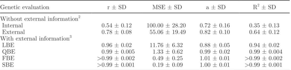
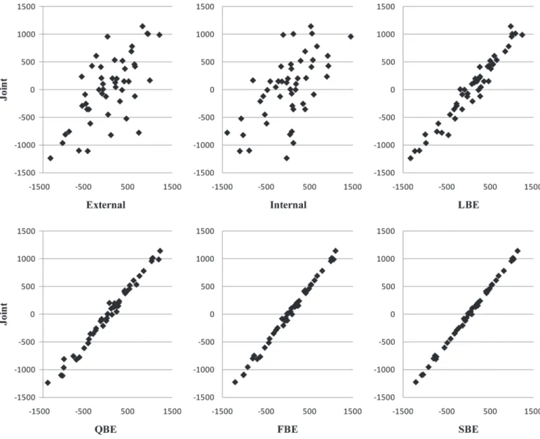
Results for r, MSE, a, and R2 illustrating the predic-tion of joint breeding values are shown in Table 2 for the external animals (i.e., the 50 external sires associ-ated with external information integrassoci-ated through a Bayesian evaluation), and in Table 3 for all the internal animals (i.e., animals associated with only internal information). To visualize effects of the integration of external information, EBV of the 50 external animals for one randomly chosen simulation are plotted in Fig-ure 1.
First, concerning the 50 external animals, rank cor-relations between joint evaluation and the 4 Bayesian implementations increased at least by 43% to be >0.96. Therefore, the integration of external information led to an improved ranking of external animals in the in-ternal evaluation (i.e., more similar ranking compared with the ranking of the joint evaluation), which was expected, especially by Legarra et al. (2007) and Quaas and Zhang (2006). Concerning all the internal animals, even if rank correlations increased only by 4%, integra-tion of external informaintegra-tion for external animals related to the internal population led to rank internal animals almost identically to their ranking obtained with the joint evaluation.
Second, according to the 4 estimated parameters r, MSE, a, and R2, the integration of external information for the 50 external animals led to better predictions of the joint evaluation through all Bayesian implementa-tions for all 50 external animals as well as for all inter-nal animals. However, whereas integrated exterinter-nal
in-1520 VANDENPLAS AND GENGLER
Journal of Dairy Science Vol. 95 No. 3, 2012
formation was identical for the 4 Bayesian implementa-tions, significant differences were found among the 4 Bayesian procedures concerning prediction accuracy for breeding values. Breeding value prediction compared with the reference method (i.e., the joint evaluation) was poorest for the LBE method for the 50 external animals as well as for the internal animals. This can be explained by the approximation of the matrix D by LBE. It approximates the latter matrix by a diagonal matrix in which diagonal elements are equal to PEV, ignoring prediction error covariances associated with
every external evaluation. In contrast, the 4 parameters associated with FBE and SBE showed that integration of all relationships between the 50 external animals and all the internal animals for the approximation of D al-lowed the propagation of external information through the whole pedigree. Consequently, internal animals re-lated to their external relatives were predicted better, too. This propagation is not possible in current meth-ods based on selection index theory (VanRaden, 2001; Gengler and VanRaden, 2008), where information is combined on an animal-by-animal basis. Therefore,
Table 2. Rank correlations (r) and mean squared errors (MSE) expressed as a percentage of the internal MSE between joint evaluation and an external evaluation, an internal evaluation, and 4 different Bayesian procedures, regression coefficients (a), and coefficients of determination (R2) of the regression of the joint evaluation on the 6 other evaluations1
Genetic evaluation r ± SD MSE ± SD a ± SD R2 ± SD
Without external information2
Internal 0.54 ± 0.12 100.00 ± 28.20 0.72 ± 0.16 0.35 ± 0.13 External 0.78 ± 0.08 55.06 ± 19.49 0.82 ± 0.10 0.64 ± 0.12 With external information3
LBE 0.96 ± 0.02 11.76 ± 6.32 0.88 ± 0.05 0.94 ± 0.02
QBE 0.99 ± 0.005 1.33 ± 0.62 0.99 ± 0.02 0.99 ± 0.004
FBE >0.99 ± 0.002 0.49 ± 0.25 1.01 ± 0.01 >0.99 ± 0.002 SBE >0.99 ± 0.001 0.19 ± 0.09 1.00 ± 0.01 >0.99 ± 0.001
1
All data are presented for external animals associated to external information integrated through a Bayesian evaluation. Reported results are averages and standard deviations over 100 replicates.
2
Internal = internal genetic evaluation; external = external genetic evaluation.
3LBE = Bayesian evaluation following Legarra et al. (2007) and using external EBV and prediction error
vari-ances (PEV) associated with external sires obtained from the external evaluation. QBE = Bayesian evaluation following Quaas and Zhang (2006) and using external EBV and PEV associated with external sires obtained from the external evaluation. FBE = Bayesian evaluation using external EBV and PEV associated with exter-nal sires obtained from the exterexter-nal evaluation where exterexter-nal EBV for all interexter-nal and exterexter-nal animals were predicted and used. SBE = Bayesian evaluation using external EBV and PEV associated with external sires obtained from the external evaluation where external EBV for all internal and external animals were predicted and used and the double counting among external animals was avoided.
Table 3. Rank correlations (r) and mean squared errors (MSE) expressed as a percentage of the internal MSE between joint evaluation, and an internal evaluation and 4 different Bayesian procedures, and regression coefficients (a), and coefficients of determination (R2) of the regression of the joint evaluation on the 6 other evaluations1
Genetic evaluation r ± SD MSE ± SD a ± SD R2 ± SD
Without external information
Internal2 0.95 ± 0.02 100.00 ± 33.52 0.95 ± 0.03 0.91 ± 0.03
With external information3
LBE 0.99 ± 0.003 12.48 ± 6.27 0.98 ± 0.01 0.99 ± 0.01
QBE >0.99 ± 0.000 1.36 ± 0.71 1.00 ± 0.004 >0.99 ± 0.001 FBE >0.99 ± 0.000 0.79 ± 0.52 1.00 ± 0.003 >0.99 ± 0.000 SBE >0.99 ± 0.000 0.26 ± 0.23 1.00 ± 0.002 >0.99 ± 0.000
1All data are presented for internal animals associated to only internal information. Reported results are
aver-ages and standard deviations over 100 replicates.
2Internal = internal genetic evaluation. 3
LBE = Bayesian evaluation following Legarra et al. (2007) and using external EBV and prediction error vari-ances (PEV) associated with external sires obtained from the external evaluation. QBE = Bayesian evaluation following Quaas and Zhang (2006) and using external EBV and PEV associated with external sires obtained from the external evaluation. FBE = Bayesian evaluation using external EBV and PEV associated with exter-nal sires obtained from the exterexter-nal evaluation where exterexter-nal EBV for all interexter-nal and exterexter-nal animals were predicted and used. SBE = Bayesian evaluation using external EBV and PEV associated with external sires obtained from the external evaluation where external EBV for all internal and external animals were predicted and used and the double counting among external animals was avoided.
FBE and SBE have here a clear advantage compared with current methods. Furthermore, integration of all relationships allowed us to compute only one relation-ship matrix A−1 that takes into account all relation-ships among internal and external animals, whereas QBE needs the computation of the matrix A−EE1 as well as the matrix A−1. One can assume that numerically the setting up of A−1 using the usual rules is easier and numerically more stable than computing A−EE1for poten-tially several thousands of animals.
Third, the 4 parameters showed that the SBE led to breeding values most similar to those estimated by the joint evaluation for the external animals. Values of R2, a, and r were close to 1 with only few variation among replicates (SD <0.001). Mean squared error was the lowest of the 4 Bayesian implementations and showed that the application of TSA avoided double counting among external animals. Outliers of breeding values for external animals were limited. For the internal ani-mals, QBE, FBE, and SBE were similar following the
Figure 1. Examples from one randomly chosen simulation showing EBV of the 50 external animals between joint evaluation and external and internal evaluations, Legarra-type Bayesian evaluation [LBE; i.e., a Bayesian evaluation following Legarra et al. (2007) and using external EBV and prediction error variances (PEV) associated with external sires obtained from the external evaluation], Quaas-type Bayesian evaluation [QBE; i.e, a Bayesian evaluation following Quaas and Zhang (2006) and using external EBV and PEV associated with external sires obtained from the external evaluation], first version of modified Bayesian evaluation (FBE; i.e., a Bayesian evaluation using external EBV and PEV associated with external sires obtained from the external evaluation where external EBV for all internal and external animals were predicted and used), and second version of modified Bayesian evaluation (SBE; i.e., a Bayesian evaluation using external EBV and PEV associated with external sires obtained from the external evaluation where external EBV for all internal and external animals were predicted and used and the double counting among external animals was avoided).
1522 VANDENPLAS AND GENGLER
Journal of Dairy Science Vol. 95 No. 3, 2012
4 parameters. Nevertheless, MSE was the lowest for SBE and showed the importance of the double counting among external animals on internal animals. However, with regards to r, a, and R2 for the external and the internal animals estimated by FBE, double counting could be ignored if contributions due to relationships are low compared with contributions due to own re-cords. If this is not the case, as for genomic informa-tion, TSA should be applied.
Fourth, no assumption was made about the differ-ence of the amount of information between external and internal information. An external animal could get more information from the internal than from the external data. Integration of external information led to better predictions for breeding values obtained by the joint evaluation. Therefore, integration of external information seems to be important even if the amount is low.
Finally, the developed methods could be used in different settings. Many situations exist where local (internal) evaluations would benefit from the integra-tion of external informaintegra-tion (e.g., Gengler and Vand-erick, 2008). Because the developed methods can be used for multi-trait and other complex models, they allow the use of external information to improve the accuracy of evaluations for correlated, but only locally available traits as fine milk composition traits, such as free fatty acids, milk proteins, and other minor constituants (e.g., Gengler et al., 2010). In the context of genomic selection, integration of external genomic information into routine genetic evaluations could be done using the proposed methods after some adapta-tions (e.g., Gengler and Verkenne, 2007). Furthermore, as an anonymous reviewer reported, the matrix G*−1 is very similar to the inverse of the matrix H used in the single-step genomic evaluations and included both pedigree-based relationships and differences be-tween pedigree-based and genomic-based relationships (Aguilar et al., 2010; Christensen and Lund, 2010). In a different setting and after taking precautions to avoid double counting because of the use of the same data, regular genetic evaluation results from a larger popula-tion could also be used as external priors in gene effect discovery studies (e.g., Buske et al., 2010) or any other studies requiring accurate estimation of a polygenic ef-fect jointly with marker, SNP, or gene efef-fects.
CONCLUSIONS
According to these results, rankings of animals were most similar to those of a joint evaluation after the in-tegration of all relationships and the application of the TSA to avoid double counting among external animals through SBE. It proved that the TSA worked well,
although the creation of the absorption matrix M did not take into account the fixed effects considered in the external evaluation, which were unknown, but only one hypothetical unobserved fixed effect. The results based on our simulation showed that the Bayesian procedures FBE and QBE also worked well, with FBE having some computational advantages. Finally, with some adapta-tions and adjustments, FBE and SBE could be applied to integrate external information into routine genetic evaluations, SBE having additional advantages but be-ing computationally more demandbe-ing.
ACKNOWLEDGMENTS
This research received financial support from the Eu-ropean Commission, Directorate-General for Agricul-ture and Rural Development, under Grand Agreement 211708 and form the Commission of the European Communities, FP7, KBBE-2007-1. This paper does not necessarily reflect the view of these institutions and in no way anticipates the Commission’s future policy in this area. Jérémie Vandenplas, research fellow, and Nicolas Gengler, senior research associate, acknowl-edge the support of the National Fund for Scientific Research (Brussels, Belgium) for these positions and for the additional grants 2.4507.02F, F4552.05, and 2.4.623.08.F. Additional financial support was provided by the Ministry of Agriculture of Walloon Region of Belgium (Service Public de Wallonie, Direction générale opérationnelle “Agriculture, Ressources naturelles et Environnement” – DGA-RNE) through research proj-ects D31-1207, D31-1224/S1, and D31-1233/S1. The authors are grateful to the University of Liège (SEGI facility) for the use of the NIC3 supercomputer fa-cilities. The authors thank the members of the Animal Breeding and Genetics Group (Animal Science Unit, Gembloux Agro-Bio Tech, University of Liège), and in particular Bernd Buske and Ryan Ann Davis (Univer-sity of Georgia, Athens) for reviewing the manuscript. Useful comments from three anonymous reviewers are also acknowledged.
REFERENCES
Aguilar, I., I. Misztal, D. L. Johnson, A. Legarra, S. Tsuruta, and T. J. Lawlor. 2010. Hot topic: A unified approach to utilize phenotypic, full pedigree, and genomic information for genetic evaluation of Holstein final score. J. Dairy Sci. 93:743–752.
Aguilar, I., I. Misztal, A. Legarra, and S. Tsuruta. 2011. Efficient com-putation of the genomic relationship matrix and other matrices used in single-step evaluation. J. Anim. Breed. Genet. 128:422– 428. doi:10.1111/j.1439-0388.2010.00912.x.
Buske, B., M. Szydlowski, and N. Gengler. 2010. A robust method for simultaneous estimation of single gene and polygenic effect in dairy cows using externally estimated breeding values as prior information. J. Anim. Breed. Genet. 127:272–279.
Christensen, O. F., and M. Lund. 2010. Genomic prediction when some animals are not genotyped. Genet. Sel. Evol. 42:2.
Colleau, J. J. 2002. An indirect approach to the extensive calculation of relationship coefficients. Genet. Sel. Evol. 34:409–421. Gengler, N., and S. Vanderick. 2008. Bayesian inclusion of external
evaluations into national evaluation system: Application to milk production traits. Interbull Bull. 38:70–74.
Gengler, N., S. Vanderick, V. Arnould, and H. Soyeurt. 2010. Genetic evaluation for milk fat composition in the Walloon Region of Bel-gium. Interbull Bull. 42:81–84.
Gengler, N., and P. M. VanRaden. 2008. Strategies to incorporate genomic prediction into populationwide genetic evaluations. J. Dairy Sci. 91(E-Suppl. 1):506. (Abstr.)
Gengler, N., and C. Verkenne. 2007. Bayesian approach to integrate molecular data into genetic evaluations. Interbull Bull. 37:37–41. Henderson, C. R. 1984. Applications of Linear Models in Animal
Breeding. 2nd ed. University of Guelph, Guelph, ON, Canada. Klei, L., R. L. Quaas, E. J. Pollak, and B. E. Cunningham. 1996.
Multiple breed evaluation. Pages 106–113 in Proc. 28th Research Symposium and Annual Meeting. Beef Improvement Federation, Birmingham, AL.
Legarra, A., J. K. Bertrand, T. Strabel, R. L. Sanchez, and I. Misztal. 2007. Multi-breed genetic evaluation in a Gelbvieh population. J. Anim. Breed. Genet. 124:286–295.
Misztal, I., A. Legarra, and I. Aguilar. 2009. Computing procedures for genetic evaluation including phenotypic, full pedigree, and ge-nomic information. J. Dairy Sci. 92:4648–4655.
Misztal, I., and G. R. Wiggans. 1988. Approximation of prediction er-ror variance in large-scale animal models. J. Dairy Sci. 71(Suppl. 2):27–32.
Mrode, R. A. 2005. Linear Models for the Prediction of Animal Breed-ing Values. 2nd ed. CABI PublishBreed-ing, WallBreed-ingford, UK.
Quaas, R. L., and Z. Zhang. 2006. Multiple-breed genetic evaluation in the US beef cattle context: Methodology. CD-ROM Commun. 24–12 in Proc. 8th World Congr. Appl. Livest. Prod., Belo Hori-zonte, Brazil.
Quaas, R. L., and Z. W. Zhang. 2001. Incorporating external informa-tion in multibreed genetic evaluainforma-tion. J. Anim. Sci. 79(Suppl. 1):342. (Abstr.)
Van Vleck, L. D. 1994. Algorithms for simulation of animal models with multiple traits and with maternal and non-additive genetic effects. Br. J. Genet. 17:53–57.
VanRaden, P. M. 2001. Methods to combine estimated breeding values obtained from separate sources. J. Dairy Sci. 84(E Suppl.):E47– E55.
Zhang, Z. W., R. L. Quaas, and E. J. Pollak. 2002. Simulation study on the effects of incorporating external genetic evaluations results. CD-ROM Commun. 20–14 in Proc. 7th World Congr. Appl. Liv-est. Prod., Montpellier, France.
1524 VANDENPLAS AND GENGLER
Journal of Dairy Science Vol. 95 No. 3, 2012
APPENDIX
Equivalence of Mixed Model Equations Considering the Estimation of Base Differences
Assume that external information is available for both internal and external animals from a joint genetic evaluation of all internal and external animals based only on external data and that the vectors of the base dif-ferences between the internal genetic evaluation and the joint genetic evaluation are ˆbE for the external animals and ˆbI for the internal animals. Therefore, the Bayesian mixed model equations [1] can be written as
X R X X R Z X R Z 0 0 Z R X Z R Z G I I1 I I I1 IE I I1 II IE I1 I IE I1 IE EE ′ ′ ′ ′ ′ − − − − − + + Λ GG (G )U G U Z R X G Z R Z G G U G U 0 U EI EE E EI I II I1 I IE II I1 II II IE E II I + + − − Λ ′ ′ ′′ ′ ′ ′ ′ ′ ′ E EE E EI E EE E E EI I I IE I II I IE E (G ) U G U (G )U U G U 0 U G U G U G U U +Λ +Λ ′′I II I I E I E I G U u u b b ⎡ ⎣ ⎢ ⎢ ⎢ ⎢ ⎢ ⎢ ⎢ ⎢ ⎢ ⎢ ⎤ ⎦ ⎥ ⎥ ⎥ ⎥ ⎥ ⎥ ⎥ ⎥ ⎥ ⎥ ⎡ ⎣ ⎢ ⎢ ⎢ ⎢ ⎢ ⎢ ⎢ ⎢ ⎢ ˆ ˆ ˆ ˆ ˆ β ⎤⎤ ⎦ ⎥ ⎥ ⎥ ⎥ ⎥ ⎥ ⎥ ⎥ ⎥ = + + + − − − X R y Z R y (G ) G Z R y I I1 I IE I1 I EE E EI I II I1 I ′ ′ ′ Λ μ μ + + + + + + ⎡ ⎣ ⎢ ⎢ ⎢ ⎢ ⎢ G G U (G ) U G U G U G IE E II I E EE E E EI I I IE E I II I μ μ Λ μ μ μ μ ′ ′ ′ ′ ⎢⎢ ⎢ ⎢ ⎢ ⎢ ⎤ ⎦ ⎥ ⎥ ⎥ ⎥ ⎥ ⎥ ⎥ ⎥ ⎥ ⎥ ,
where ZIE and ZII are the incidence matrices for the external and internal animals, respectively.
Because Λ =D−1−G−EE1, GIE−G (G ) GII II −1 IE =0, GEE−G (G ) GEI II −1 IE =G−EE1, and ˆuI = −(G ) G uII −1 IEˆ ,E the de-velopment of the fourth equation leads to U D (u′E −1 ˆE−μE)+U (G′E EE+Λ)U bE Eˆ +U G U bE EI I Iˆ =0, and the
devel-opment of the fifth equation leads to U bI Iˆ = −(G ) G U bII −1 IE E Eˆ .
After absorption of the fifth equation, the vector ˆbE is estimated as ˆbE=(U D U ) U D (′E −1 E −1 ′E −1 μE−u )ˆE . Fur-thermore, it can be shown that GIEμE+GIIμI = and (G0 EE+Λ μ) E+GEIμI =D−1μ . The equivalent mixed E model equations can be written as
X R X X R Z X R Z 0 Z R X Z R Z G G I I1 I I I1 IE I I1 II IE I1 I IE I1 IE EE ′ ′ ′ ′ ′ − − − − − + + Λ EEI 1 E II I1 I IE II I1 II II E 1 E 1 E D U Z R X G Z R Z G 0 0 U D 0 U D U − − − − − + ⎡ ⎣ ⎢ ⎢ ⎢ ′ ′ ′ ′ ⎢⎢ ⎢ ⎢ ⎢ ⎢ ⎤ ⎦ ⎥ ⎥ ⎥ ⎥ ⎥ ⎥ ⎥ ⎥ ⎡ ⎣ ⎢ ⎢ ⎢ ⎢ ⎢ ⎢ ⎢ ⎤ ⎦ ⎥ ⎥ ⎥ ⎥ ⎥ ⎥ ⎥ = − ˆ ˆ ˆ ˆ βI E I E I I1 I u u b X R y Z ′ ′IIE I1 I 1 E II I1 I E 1 E R y D Z R y U D − − − − + ⎡ ⎣ ⎢ ⎢ ⎢ ⎢ ⎢ ⎢ ⎢ ⎢ ⎤ ⎦ ⎥ ⎥ ⎥ ⎥ ⎥ ⎥ ⎥ ⎥ μ μ ′ ′ .
Elimination of Base Difference Equations in FBE and SBE
The derivation is based on the estimation of ˆu+Ubˆ instead of ˆu and ˆb separately. The associated mixed model equations can be obtained through a few steps. First, using some rearrangements, the development according to the first, second, and third lines of the Bayesian mixed model equation [1] leads to, respectively:
X R X′I −I1 I Iβˆ +X R Z u′I −I1 I
(
ˆ+Ubˆ)
=X R′I −I1(
yI +Z UbI ˆ ,)
[A1]Z R X′I −I1 I Iβˆ +
(
Z R Z′I −I1 I+G* 1−)
(
uˆ+Ubˆ)
−G* 1−μ0 =Z R′I −I1(
yI +Z UI ˆˆ ,b)
[A2] U G′ * 1−(
ˆu+Ubˆ)
−U G′ * 1−μ0 =0. [A3]Therefore, solutions for ˆu+Ubˆ and ˆb can be obtained by solving jointly [A4] and [A5]: X R X X R Z Z R X Z R Z G u U I I1 I I I1 I I I1 I I I1 I * 1 I ′ ′ ′ ′ − − − − + − ⎡ ⎣ ⎢ ⎢ ⎢ ⎤ ⎦ ⎥ ⎥ ⎥ + ˆ ˆ β ˆ ˆ ˆ ˆ b X R y Z Ub Z R y Z Ub G I I1 I I I I1 I I * 1 0 ⎡ ⎣ ⎢ ⎢ ⎢ ⎤ ⎦ ⎥ ⎥ ⎥= +
(
)
+(
)
+ ⎡ ⎣ ⎢ − − − ′ ′ μ ⎢⎢ ⎢ ⎢ ⎤ ⎦ ⎥ ⎥ ⎥ ⎥ , [A4] U G′ * 1−Ubˆ=U G′ * 1−(
μ0−uˆ .)
[A5]If all the animals contribute to the base differences, then U represents a summing matrix and ˆb the vector of
weighted average base differences between μ0 and ˆ.u Given this, Ubˆ represents a vector of constants added to each EBV and Z UbI ˆ represents a vector of constants added to each record. Therefore, the following reparameterization can be used: ˆu* = +ˆu Ubˆ.
Furthermore, adding the same constants to each EBV will not change the rankings, and rankings will be thereby invariant to the used constants. The constants added to the records will also only change estimates of fixed effects. Those different estimates of fixed effects will have no effect on animal rankings because all animals are affected by the same constant. For these reasons, [A4] can be rewritten as follows:
X R X X R Z Z R X Z R Z G u I I1 I I I1 I I I1 I I I1 I * 1 I ′ ′ ′ ′ − − − − + − ⎡ ⎣ ⎢ ⎢ ⎢ ⎤ ⎦ ⎥ ⎥ ⎥ ˆ ˆ * * β ⎡⎡ ⎣ ⎢ ⎢ ⎢ ⎤ ⎦ ⎥ ⎥ ⎥= + ⎡ ⎣ ⎢ ⎢ ⎢ ⎤ ⎦ ⎥ ⎥ ⎥ − − − X R y Z R y G I I1 I I I1 I * 1 0 ′ ′ μ ,
where ˆβI* represents the new fixed effects computed by ignoring the constant in the records.
TSA
The estimation of RE independent from contributions due to relationships or correlated traits is performed by the following TSA; the TSA must be repeated for each trait.
The first step of the TSA is solved iteratively as follows: (1) For each animal i, H
1 0
ii REij
[ ] = , where H
1 is a diagonal matrix with RE of each external animal i based on the external PEV for the jth trait.
(2) Q1[ ]1 =H1[ ]0. (3) k = 1.
(4) P[ ]k =
(
Q[ ]1k +A*−1)
−1
λj , where A*−1 is the inverse of the relationship matrix that accounts for the relation-ships between external animals and their ancestors and λj e
u j j =σ σ 2 2 for with σej 2 and
σu2j are the error variance
and the genetic variance for the jth trait, respectively. (5) H2[ ]k P[ ]k I − =⎛⎝⎜⎜⎜diag diag
(
( )
)
⎞⎠⎟⎟⎟ − 1 λ. (6) S[ ]k =H[ ]10 −H[ ]2k.(7) If S[ ]k is not sufficiently small, perform for each animal i: (a) Q[1k 1ii+]=Q[ ]1kii +S[ ]k.
(b) If any diagonal element in Q1 k 1+
[ ] is negative, set it to 0.
(c) k = k + 1. (d) Repeat from (4). (8) For each animal i, perform: (a) Xi = 1 if Q[ ]1kii ≠ 0. (b) Xi = 0 if Q1[ ]kii = 0.
1526
Journal of Dairy Science Vol. 95 No. 3, 2012
(9) M=Xd−X X X
(
′)
−1X′, where the matrix M is the absorption matrix based on the contributions due to own records.The second step of the TSA is solved iteratively as follows: (1) For each animal i, H10
ii REij [ ] = (2) Q2[ ]1 = H1[ ]0 *M* H1[ ]0. (3) k = 1. (4) P[ ]k =
(
Q[ ]2k +A*−1)
− 1 λj . (5) H2[ ]k P[ ]k I − =⎛⎝⎜⎜⎜diag diag(
( )
)
⎞⎠⎟⎟⎟ − 1 λ. (6) S[ ]k =H[ ]10 −H[ ]2k.(7) If S[ ]k is not sufficient small, perform for each animal i: (a) Q[2k 1ii+]=Q[ ]2kii+S[ ]k.
(b) If any diagonal element in Q[k 1+] is negative, set it to 0. (c) Q[2k 1ij+]= Q[2k 1ii+]*M−ii1 *Mij* M−jj1*Q[2k 1jj+].
(d) k = k + 1. (e) Repeat from (4).
(8) If Q2[k 1+] and Q[ ]2k are close enough, perform for each animal i, RE*j Q2k 1 M 1
ii = ii ii
+
[ ]* − , where RE
j
* is a diagonal matrix with diagonal elements equal to RE only due to own records for the jth trait.