Proceedings of the ICTWS 2014 7th International Conference on Thin-Walled Structures ICTWS2014 28 September – 2 October 2014, Busan, Korea
ICTWS2014-0904
A SIMPLIFIED PROCEDURE TO ASSESS THE DYNAMIC PRESSURES ON LOCK
GATES
Loïc Buldgen, Afshin Gazerzadeh, Andreea Bela, Philippe Rigo University of Liège,
Liège, Belgium
Hervé Le Sourne
Institut Catholique d'Arts et Métiers de Nantes, Nantes, France
ABSTRACT
The paper is concerned with the seismic design of lock gates. During an earthquake, it is evident that the liquid contained in the lock chamber is responsible for an additional hydrodynamic pressure acting on the structure. This one is known to have three different contributions, which are respectively called the convective, rigid and flexible impulsive parts. The two first ones have already been extensively studied in the literature and are quite easy to evaluate. Nevertheless, characterizing the flexible contribution is more difficult, as it is largely influenced by the coupling occurring between the fluid and the gate. The only relevant way to overcome this difficulty seems to resort to finite elements software, which is not always convenient. Therefore, some research have been undertaken to provide a rapid meshless method leading to an approximation of the flexible pressure on lock gates. As detailed in the present paper, this is achieved by applying an analytical approach based on the virtual work principle. As a matter of validation, the results obtained analytically are compared to numerical solutions. The agreement between both of them is found to be satisfactory.
1. INTRODUCTION
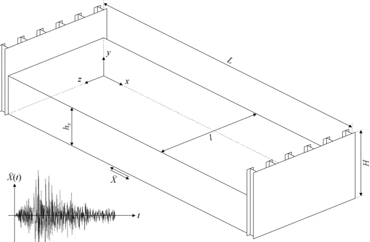
As depicted on Figure 1, we consider a basic lock chamber made of two identical downstream and upstream gates, having a height H and a width l. These two structures are separated by a certain distance L corresponding to the total length of the lock chamber. This one is filled with water up to a level hs.
During an earthquake, this configuration is submitted to three different seismic acceleration components respectively applied along the x, y and z axes. In this paper however, the effect of the vertical and transversal contributions will not be considered, so only the longitudinal acceleration applied along the x axis will be investigated here. This one is denoted by Ẍ(t) and is assumed to exhibit the typical time evolution represented on Figure 1.
As the structure is submitted to the ground acceleration Ẍ(t), an additional hydrodynamic pressure is applied on the gates. This phenomenon is due to the fact that the water confined between the gates is also accelerated. The resulting
total pressure is known to have the three different following contributions:
The convective part, which is coming from the sloshing appearing at the free surface of the lock chamber. This wave motion is responsible for a water pressure that is said to be convective.
The rigid impulsive part, which is derived under the assumption of perfectly rigid gates. With this hypothesis, the structure is supposed to move in unison with the ground without exhibiting any vibration. This rigid-body motion results in a water pressure that is said to be rigid impulsive. The rigid flexible part, which is coming from the fact that the gates are not ideal rigid structures and therefore superimpose their own vibrations to the basic ground accelerations. This movement also produces an additional water pressure that is said to be flexible impulsive.
The two first contributions have already been extensively studied in the literature. Many developments are therefore
available, such as those performed by Housner (1974), Ibrahim (2005), Haroun (1984) or Epstein (1976) amongst others. All these authors provide various analytical formulae for deriving the rigid and convective pressures. Nevertheless, dealing properly with the third contribution is more difficult. This is due to the fact that the flexible pressure is directly influenced by the vibrations of the gate, which turns out to have consequences on the dynamic response of the structure itself. This means that there is a coupling between the own accelerations of the gate and the pressure acting on it. Solving analytically this kind of fluid-structure interaction problem is almost impossible, so it is of current practice to resort to finite elements methods to get numerical solutions.
Even if this kind of software constitutes a precious tool for engineers, finite elements also have some drawbacks. Indeed, to perform coupled fluid-structure analyses, it is of course required to model both the liquid and the gates, but such an approach may be time demanding because it is not easy to develop a consistent model for the fluid. Moreover, the calculation time may become prohibitively long if the liquid domain has to be entirely represented, in particular in very large structures such as lock chambers. This way of working is of course not well-suited when engineers are still pre-designing a structure because they do not necessarily have time
to perform heavy calculations. For all the aforementioned reasons, it is clear that another approach is required to include the seismic effect in the early design of lock gates, particularly if these structures are located in sensible areas.
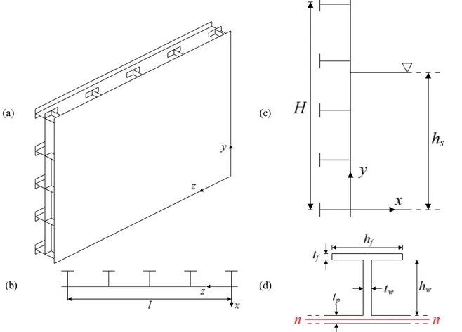
Exposing a new simplified method is precisely the goal of the paper. In this article, we consider the case of a lock gate having a single plating and an orthogonal stiffening system, as depicted on Figure 2(a). The vertical reinforcing elements (oriented along the y axis, Figure 2(b)) are called the frames, while the horizontal reinforcing ones (oriented along the z axis, Figure 2(c)) are called the girders. In addition to this basic system, some supplementary horizontal and/or vertical smaller stiffeners may be added to reinforce the portion of the plating located between two frames and two girders. All these components have a T-shaped cross-section (Figure 2(d)). The web height and thickness are respectively denoted by hw and tw,
while the flange width and thickness are designated by hf and
tf.
Regarding the boundary conditions of the gate, it is worth mentioning that the structure is assumed to be simply supported along the two lines located in z = 0 and z = l. On the contrary, the top and bottom edges in y = H and y = 0 are free to move.
(a) (c)
(b) (d)
Figure 2. Three dimensional view of a simple gate; Longitudinal view of the lock chamber. 2. FREE VIBRATION ANALYSIS OF A DRY GATE
2.1 Analytical Derivation
The first step in the seismic analysis is to find the modal properties of the dry structure. In other words, our goal now is to get an analytical approximation of the natural frequencies ωi and mode shapes δi characterizing the gates without
considering the water present in the lock chamber. To do so, we will follow the Rayleigh-Ritz method. This approach is extensively described by Shames [9] and has been successfully applied in references [1, 7, 10] to derive the vibration properties of stiffened plates in various circumstances.
To apply the Rayleigh-Ritz procedure, we first need to decompose the mode shapes δi as a set of admissible functions
ψj. Consequently, we have:
M j j ji i y z v y z 1 , ,
(1)where vji are unknown coefficients and M is the number of
terms used in the decomposition process. The functions ψj may
be arbitrarily chosen, provided that they satisfy the boundary conditions detailed in section 1. In this paper, we propose the following combination: ) ( ) ( ) , (y z fj y gj z j
(2)in which fj and gj are some functions characterizing the
free vibrations of the vertical and horizontal reinforcing elements respectively. As the gate is always supported along the edges z = 0 and z = l, it seems reasonable to choose gj as
being the eigenmodes of a doubly supported beam with a span l. Similarly, as the structure is free along the horizontal lines y = 0 and y = H, it may be convenient for fj to consider the mode
shapes of a free-free beam. In the literature, it is easy to find that:
z z g y B y B y f y y y f y f y f A y f j j j j j j j j j j j j j j sin ) ( cosh cos ) ( sinh sin ) ( ) ( ) ( ) ( ) 2 ( ) 1 ( ) 2 ( ) 1 ( (3)where Aj is the modal amplitude. The parameters λj, γj and Bj
are found to satisfy the following equations:
jH
cosh
jH
1 j nj /l
cos
1,2...
cosh sin sinh j j j j j j n H H H H B
(4b)Finally, we see that Eq. (2) and (3) allow us to find a set of admissible functions ψj. These ones may then be introduced in
Eq. (1) to get the approximate decomposition of the eigenmodes characterizing the dry gate. Once this operation is achieved, the second step in the Rayleigh-Ritz method is to evaluate the internal and kinetic energies U and T associated to the structural vibrations. According to Shames [9], U may be seen as the sum of two contributions Up and Ur. The first one is
coming from the plating, while the second one is due to the reinforcing system. It may be shown [9] that:
n H n i n v r n l n i n h r r r r i i i p A p i i p dy z y y EI U dz z y z EI U U U U z y z y U dydz U z y U 0 2 2 2 , ) 2 ( 0 2 2 2 , ) 1 ( ) 2 ( ) 1 ( 2 2 2 2 2 2 * * 2 2 2 2 2 2 , 2 , 2 1 2 2 (5)where ν and E are respectively the Poisson ratio and Young modulus. The plate is characterized by its surface A and bending flexibility D, while the horizontal and vertical reinforcing elements have a T-shaped cross section with an inertia designated by Ih,n and Iv,n. It is worth noting that these
latter are calculated with respect to the neutral bending axis of the plating (see the line n-n on Figure 2(d)). Finally, in Eq. (5), yn and zn denotes the discrete locations occupied by the
stiffeners along the y vertical and z horizontal axes.
Similarly, the kinetic energy ωi2T may also be obtained by
summing up the two individual contributions ωi2Tp and ωi2Tr
(where ωiis the eigenfrequency associated to the mode shape
δi). According to Shames [9], we have:
n H n i n v r n l n i n h r r r r A i p p dy z y A T dz z y A T T T T dydz z y t T 0 2 , ) 2 ( 0 2 , ) 1 ( ) 2 ( ) 1 ( 2 , 2 , 2 , 2 (6)where ρ is the mass density and tp the plate thickness. Ah,n and
Av,n are the cross section areas of the horizontal and vertical
stiffeners.
In order to find the unknown coefficients vji appearing in
Eq. (1), we may further introduce this expression in Eq. (5) and Eq. (6). This operation is quite fastidious and leads to a matrix formulation for U and T. After performing all the calculation, it can be shown that:
i T i M j M k ki jk ji i T i M j M k ki jk ji v U v v U v U v T v v T v T 2 1 2 1 2 1 2 1 1 1 1 1
(7)where vi is a vector containing vji. The terms Tjk and Ujk
associated to the matrices [T] and [U] may be found by introducing Eq. (1) in Eq. (5) and Eq. (6). They are defined by the expressions detailed in the Appendix. With these results, the final step in the procedure is then to evaluate the Rayleigh quotient R. This one is simply defined by:
i T i i T i v U v v T v R (8)in which the unkwnown coefficients contained in vi are to be
found by minimizitation of R. As detailed in [9], this last operation is achieved by solving the following classical problem:
0
0det U i2 T U i2 T vi (9)
2.2 Numerical Validation
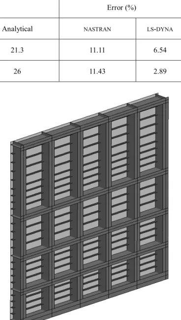
In order to corroborate the analytical developments realized in the previous sections, we can compare them with finite element analyses. The idea is to check if the theoretical prediction of the main eigenfrequencies of a chosen gate sticks to the solutions obtained numerically. For the conciness of the paper, we will limit our presentation to the case of the gate depicted on Figure 3. This structure has a square plating, with H = l = 13.1 m and a thickness tp of 1.2 cm. It is reinforced by
six vertical frames and five horizontal girders. The first ones are regularly placed over the width l, with a spacing of 2.62 m. The disposition of the girders is not regular, as the reinforcement is more important near the bottom of the gate. Some smaller horizontal stiffeners are also present. The geometrical and material properties are summarized in Tables 2 and 3.
The modal properties of the gate are obtained numerically by using the software NASTRAN. To do so, the plating is modeled by using isoparametric shell elements, while classical beam elements are used for the reinforcing system.
The modal analysis realized with NASTRAN shows that the gate has only two dominant global modes and a great amount of local ones. The natural frequencies derived by the simplified procedure of section 2.1 and the values given by NASTRAN are listed in Table 1 for these two first modes of vibration. An estimation made by the software LS-DYNA is also provided in this table. We see that the agreement is quite satisfactory. This is particularly true if we consider the results of LS-DYNA, for which the maximal relative error is not exceeding 7 %. The
discrepancy with NASTRAN is a bit more important, as an error of 12 % may be reached.
From, Table 3 it transpires that the analytical approach tends to overestimate the natural frequencies. This observation may be justified mathematically (Shames and Dym 1995), as the Rayleigh-Ritz method always gives an upper estimation of the eigenvalues.
Table 1. Comparison of the natural frequencies obtained numerically and analytically
Mode Frequency (Hz) Error (%)
/ NASTRAN LS-DYNA Analytical NASTRAN LS-DYNA
1 19.17 19.99 21.3 11.11 6.54
2 23.33 25.27 26 11.43 2.89
Table 2. Properties of the reinforcing system Horizontal girders hw (m) 0.980 tw (m) 0.020 hf (m) 0.400 tf (m) 0.025 Vertical frames hw (m) 0.980 tw (m) 0.020 hf (m) 0.500 tf (m) 0.025 Horizontal stiffeners hw (m) 0.210 tw (m) 0.006 hf (m) 0.000 tf (m) 0.000
Table 3. Material properties
Mass density ρ (kg/m³) 7850 Young modulus E (MPa) 210000 Poisson ratio ν (-) 0.3
3.DYNAMIC ANALYSIS OF LOCK GATES 3.1 Analytical Derivation
The goal of this section is to go one step further in the seismic analysis of lock gates by considering this time the situation depicted on Figure 1. Our aim is now to estimate the hydordynamic pressure acting on the structure in this case. As a first step, we can start by assuming that the out-of-plane displacements u exhibited by the gate are predominant and may be expressed as a combination of the dry eigenmodes δj
calculated in section 2.1:
N j j j t y z q t z y u 1 , ) , , (
(10)where the time coefficients qj are the unknown we have to
determine and N is the number of eigenmodes involved in the decomposition. To do so, we will apply the virtual work principle, which simply states that a necessary and sufficient condition for equilibrium is to equate the external and internal virtual works for any kinematically compatible displacements field.
Let us start by evaluating the internal virtual work δWint.
This one may still be seen as the sum of a contribution coming from the plating δWp and another one δWr due to the
reinforcing system. If we follow a similar development than the one exposed in [9], we get:
n z z H n v r n y y l n h r r r r p p p A p p p p n n dy y u y u EI W dz z u z u EI W W W W z y u z y u W y u z u z u y u W z u z u y u y u W dydz W W W D W 0 2 2 2 2 , ) 2 ( 0 2 2 2 2 , ) 1 ( ) 2 ( ) 1 ( 2 2 ) 3 ( 2 2 2 2 2 2 2 2 ) 2 ( 2 2 2 2 2 2 2 2 ) 1 ( ) 3 ( ) 2 ( ) 1 ( 1 2
(11)where δu is the virtual displacements field obtained by taking the incremental form of Eq. (10) and by involving the virtual coefficients δqk:
N k k k t y z q t z y u 1 , ) , , ( (12)On the other hand, the external virtual work δWext has to
be calculated by considering all the forces acting on the structure. In the present application, we will only consider the following ones:
The inertia forces associated to the plating and to the reinforcing system. For a given virtual displacement δu, their contribution to the external work δWext is given by:
n z H n v n y l n h A p n n dy X u u A dz X u u A dydz X u u t 0 , 0 ,
(13 ) The damping forces associated to the mass and to the stiffness of the gate. These ones are simply denoted by fd
(which is a force by unit of surface) and may be expressed as a functions of the velocity field. However, in this paper, we will not go into more details and we will simply write the external work done by fd in the following way:
dydz t z y u t z y f A d
( , , )
( , , ) (14) The pressure forces coming from the water in contact with the gate. As stated in section 2.1, the impulsive pressure is the sum of the rigid and flexible contributions. These ones are denoted by pr and pf and are responsible for the
subsequent work:
p y t p y z t
u y z t dydz A f r
( , ) ( , , )
( , , ) (15)In Eq. (15), it is worth noting that the time evolution of pr is
ruled by the ground acceleration Ẍ, while the time dependence of pf is directly related to the own accelerations ü
and δü of the gate. Some detailed expressions for pr and pf
may be found in the literature and are reported in the Appendix.
In order to find the unknown coefficients qj mentioned in
Eq. (10), the next step is now to replace u and δu by their expressions given by Eq. (10) and Eq. (12). This operation is quite fastidious. For the sake of simplicity, we will simply mention that doing so leads to a matrix form for δWint and
jk jk jk jk jk jk N k k N j jk j jk j k ext N k N j jk j k J M M K M C X P C q M q q W K q q W
* 1 1 * 1 1 int
(16)where α and β are the classical coefficients used for a Rayleigh-type damping. The other terms are defined by the next expressions:
M s k sk k M r M s sk rs rj jk M r M s sk rs rj jk M r M s sk rs rj jk V v P v W v J v U v K v T v M 1 1 1 1 1 1 1 (17)in which the matrices [T] and [U] have been introduced in section 2.1. The matrix [W] and the vector V may be calculated with help of the relations provided in the Appendix. In Eq. (17), it is worth noting that the matrices [M] and [K] associated to Mjk and Kjk may be seen as the usual
mass and stiffness terms characterizing the lock gate. In a similar way, the vector P related to Pk includes the effect of
the rigid pressure pr, while the matrix [J] based on Jjk
translates the action of the flexible pressure pf.
Finally, if we equate the internal and external virtual works by considering their expressions given in Eq. (16), we get:
M W
q
M
K
q
K qPX (18) where q contains the unknown terms qj. For a given timeevolution of Ẍ, this equation may be solved by applying the classical Newmark integration scheme for example. Doing so leads to the coefficients qj, which may be introduced in Eq.
(10) to find the displacements u characterizing the seismic behavior of the gate. These ones may then be used in Eq. (A1) to find the total pressure acting on the structure.
3.2 Numerical Validation
The goal of this section is to check if the analytical procedure detailed here above may lead to a reasonable approximation of the total hydrodynamic pressure induced on a lock gate during a seism. To do so, we will consider a lock chamber with a total length L of 50 m and filled with water up to a level hs of 8 m.
The numerical analyses are performed using the software LS-DYNA. The fluid is modeled as an elastic medium, with constant stress solid elements [3] affected by a fluid material law with no shearing. The mesh of the fluid domain is regular, with an approximate size of 19 × 19 × 19 cm.
The upstream and downstream gates are identical and depicted on Figure 3. The plating is modeled with Belytschko-Tsay shell elements (Hallquist 2006). To reduce a little bit the size of the model, the reinforcing system is not explicitly represented with shell elements, but rather with Hughes-Liu beams (Hallquist 2006).
The two previous entities do not share any node in common, which means that the fluid nodes are distinct from the solid ones. The LS-DYNA contact algorithm is then used to simulate the interaction between the plate and the surrounding liquid. This allows the fluid to slide on the flexible walls without friction, but prevent it from passing through the structure.
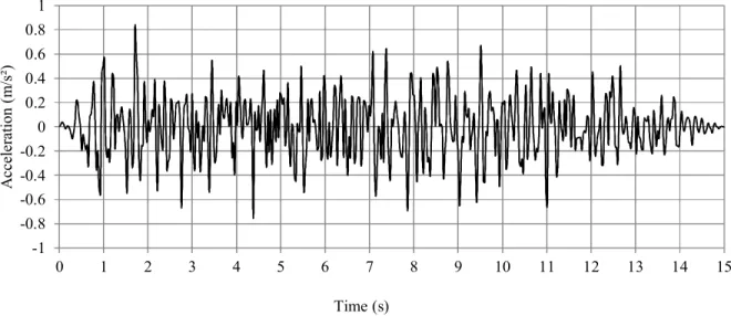
The boundary conditions are as described in section 1 and the supports are submitted to the longitudinal acceleration Ẍ of Figure 4.
As a matter of validation, we can compare the analytical prediction of the time evolution charecterizing the total resulting hydrodynamic pressure force applied on the gate with the solution calculated by LS-DYNA. The results are
plotted on
Figure 5 from which we can see that there is a quite good agreement between the two curves. From this picture, it transpires that the two solutions sometimes tends to be out-of-phase and that the analytical curve tends to be greater than the numerical one. However, this is conservative as it means that the total resulting pressure force applied on the gate is overestimated.
-1 -0.8 -0.6 -0.4 -0.2 0 0.2 0.4 0.6 0.8 1 0 1 2 3 4 5 6 7 8 9 10 11 12 13 14 15 A cc el er at io n ( m /s ²) Time (s)
Figure 4. Time evolution of the longitudinal acceleration Ẍ applied to the gate.
-2000 -1500 -1000 -500 0 500 1000 1500 2000 0 0.5 1 1.5 2 2.5 3 3.5 4 4.5 5 5.5 6 6.5 7 R e su lt in g f o rc e ( k N ) t (s) LS-DYNA Analytical -2500 -2000 -1500 -1000 -500 0 500 1000 1500 2000 2500 7 7.5 8 8.5 9 9.5 10 10.5 11 11.5 12 12.5 13 13.5 R es u lt in g f o rc e (k N ) t (s)
4.CONCLUSIONS
The main conclusions are:
1. In this paper, we presented a consistent analytical procedure to estimate the modal properties of a plane lock gate having a single plating and a simple reinforcing system.
2. The dry modal properties of the gate derived analytically have been compared with those obtained by performing simulations using the finite elements code NASTRAN. The agreement on the natural vibration frequencies was found to be satisfactory. 3. We also presented a consistent analytical procedure
to derive the hydrodynamic pressure applied on a flexible lock gate.
4. These developments were also corroborated by comparing them with solutions provided by using the finite elements code LS-DYNA.
5. The simplified methodology exposed in this paper allows for a rapid estimation of the hydrodynamic pressure applied on a lock gate, without having to perform heavy numerical simulations.
6. It is therefore well-suited for integrating the seismic action in the pre-design of lock gates.
REFERENCES
Amiri, S.N. and Esmaeily, A., 2010, Prediction of Dynamic Response of Stiffened Rectangular Plates Using Hybrid Formulation, Journal of Engineering Science and Technology, Vol.5(3), pp.251-263.
Epstein, H.I., 1976, Seismic Design of Liquid Storage Tanks, Journal of the Structural Division, Vol.102(9), pp.1659-1673.
Hallquist, J.O., 2006, LS-DYNA theoretical manual, Livermore Software Technology Corporation, Livermore, United Kingdom.
Haroun, M.A., 1984, Stress Analysis of Rectangular Walls under Seismically Induced Hydrodynamic Loads, Bulletin of Seismological Society of America, Vol.74(3), pp.1031-1041.
Housner, G.W., 1974, Dynamic Pressures on Accelerated Fluid Containers, Bulletin of Seismological Society of America, Vol.47(1), pp.15-37.
Ibrahim, R.A., 2005, Liquid Sloshing Dynamics: Theory and Applications, Cambridge University Press, Cambridge, United Kingdom.
Iyengar, K.T. and Narayana, R., 1967, Determination of the Orthotropic Plate Parameters of Stiffened Plates and Grillages in Free Vibration, Applied Sciences Research, Vol.17(6), pp.422-438.
Kim, J.K., Koh, K.H. and Kwahk, I.J., 1996, Dynamic Response of Rectangular Flexible Fluid Containers, Journal of Engineering Mechanics, Vol.122(9), pp.807-817. Shames, I.H. and Dym, C.L., 1995, Energy and Finite
Element Methods in Structural Mechanics, New Age International Publishers, India.
Zeng, H. and Bert, C.W., 2001, Free Vibration Analysis of Discretely Stiffened Skew Plates, International Journal of Structural Stability and Dynamics, Vol.1(1), pp.125-144.
APPENDIX
In this appendix, we provide some additional formulae useful for evaluating different terms introduced in the analytical processes exposed in sections 2.1 and 3.1. Let us start by considering the expressions of the rigid and flexible impulsive pressures mentioned in section 1. In the literature [9], the following results may be found:
1 0 0 0 1 2 cos cos 2 cosh cosh 4 n m h l m n mn f n n s n n f r s dydz z y u C p X L h y L p
(A1)where αn = (2n − 1)π/2hs, βn = (2n − 1)π/L, κm = mπ/L and ρf is the fluid density. The coefficient Cmn is expressed as:
2 2 2 cos cos sinh cosh 1 2 n m mn n m mn m s mn mn f mn y z L l h L C
(A2)with lm = l if m = 0 and lm = l/2 if m > 0. From Eq. (A1), we see that the rigid impulsive term pr is not dependant from the proper
displacements u of the gate, while it is not the case for the flexible part pf. This means that the fluid-structure coupling is directly
coming from pf and not from pr. Let us now introduce the mathematical equations leading to the matrices used in section 3.1. The
n H n k n v n l n k n h A k p A n n s n n k k k mn m n j mn mn m s mn mn f jk n H n jk n v n l n jk n h A jk jk n H n jk n v n l n jk n h A jk p jk dy z y A dz z y A dydz z y t L h y L V I I L l h L W dy z y h EI dz z y g EI dydz z y f D U dy z y f A dz z y f A dydz z y f t T 0 , 0 , 1 2 ) ( 1 1 ) ( 0 , 0 , 0 , 0 , ) , ( ) , ( ) , ( 2 cosh cosh 4 sinh cosh 1 2 ) , ( ) , ( ) , ( ) , ( ) , ( ) , (
(A3)where ψk are the admissible functions defined by Eq. (2). The terms fjk, gjk, hjk and Imn are defined as follow:
A n n j j mn k j jk k j jk k j j j j k k j jk dydz z y z y I y y z y h z z z y g z y z y z y z z y y z y f ) cos( cos , ) , ( ) , ( 1 2 ) , ( ) ( 2 2 2 2 2 2 2 2 2 2 2 2 2 2 2 2 2 2 2 2 2 2
(A4)With all the expressions provided in this Appendix, it is possible to apply the method exposed in section 3.1 to get an analytical estimation of the total hydrodynamic pressure pr + pf.