Robust and guaranteed output-feedback force control of piezoelectric actuator under temperature variation and input constraints

OATAO is an open access repository that collects the work of Toulouse

researchers and makes it freely available over the web where possible

Any correspondence concerning this service should be sent

to the repository administrator:

tech-oatao@listes-diff.inp-toulouse.fr

This is an author’s version published in: http://oatao.univ-toulouse.fr/27131

To cite this version:

Hammouche, Mounir and Lutz, Philippe and Rakotondrabe,

Micky

Robust and guaranteed output-feedback force control of

piezoelectric actuator under temperature variation and input

constraints. (2020) Asian J Control. 2242-2253. ISSN 2242–2253

Official URL:

Robust and guaranteed output-feedback force control of

piezoelectric actuator under temperature variation and

input constraints

Philippe Lutz

1

_{Micky Rakotondrabe}

2

Mounir

Hammouche

1

1_{FEMTO-ST Institute, Université} Bourgogne

Franche-Comté/CNRS/ENSMM, Besançon, France

2_{LGP laboratory, ENIT / Toulouse INP,} Tarbes, France

Correspondence

Micky Rakotondrabe, FEMTO-ST Institute, Université Bourgogne Franche-Comté/CNRS/ENSMM, Besançon France.

Email: mrakoton@femto-st.fr

Abstract

This paper addresses the control of manipulation force in a piezoelectric tube actuator (piezotube) subjected to temperature variation and input constrains. To handle this problem a robust output-feedback design is proposed using an interval state-space model, which permits consideration of the parameter uncer-tainties caused by temperature variation. The design method is robust in the sense that the eigenvalues of the interval system are designed to be clustered inside desired regions. For that, an algorithm based on Set Inversion Via Interval Analysis (SIVIA) combined with interval eigenvalues computation is proposed. This recursive SIVIA-based algorithm allows to approximate with subpaving the set solutions of the feedback gain [K] that satisfy the inclusion of the eigenvalues of the closed-loop system in the desired region, while at the same time ensuring the control inputs amplitude is bounded by specified saturation. The effective-ness of the control strategy is illustrated by experiments on a real piezotube of which the environmental temperature is varied.

KEYWORDS

input constraint, interval models, piezoelectric tube actuator, robust output-feedback, set inversion via interval analysis

1

INTRODUCTION

ronment and especially to ambient temperature variation [7]. Actually, there are several sources that may cause this thermal variation during experimentation: the lamps used to illuminate the tasks at the microscale and related cameras, the heating of the surrounding devices (volt-age amplifiers … ), and all other natural sources. This temperature variation considerably impacts the approxi-mated model of the actuator and induces the change in its dynamics and its steady-state behavior. Furthermore, in micro/nano manipulation, the manipulated object is usually so fragile that if the desired performance (over-shoot and rapidity) is not sufficiently respected under Piezoelectric actuators, such as a piezoelectric tube and

piezoelectric multimorph cantilever, are among the most used actuator in micro/nano-scales applications, par-ticularly in micro/nano manipulation, Scanning Probe Microscopy (SPM), and Atomic Force Microscopy (AFM) due to their high speed (large bandwidth up to 1kHz), high precision (sub-nanometric), high resolution, and multi-degrees of freedom [1–6]. Unfortunately, they are characterized by nonlinearities (hysteresis, time varying parameters, creep, etc). They are also sensitive to the

envi-this temperature variation, the manipulated object may be damaged, which makes the control of these systems not a trivial task.

Nonlinear controller design for piezoelectric actuators gained much research interest in recent decades. In these approaches, the piezoelectric actuators are approximated by uncertain nonlinear models. For instance, in [8], a nonlinear approach based on the Lyapunov function to analyze stability has been proposed. A variety of non-linear control design based on adaptive techniques are proposed in the literature [9–11]. Moreover, there are also some predictive approaches, such as the work presented in [12,13]. Further, Sliding Mode Control (SMC) design has been widely used in the literature to control piezo-electric actuators because it provides robust performances and because it has lower computational costs [14–17]. In these approaches, the hysteresis is usually divided into a linear part and a bounded time-varying unknown part. This bounded part is considered as structured uncertain-ties and is overcompensated in the control law. Other approaches based on an adaptive sliding mode controller are proposed in [17–19]. Robust control techniques have also been developed when the models of the piezoelec-tric actuators are linear with uncertainties [20–22]. For instance, in [23,24], interval techniques have been used to derive a transfer function model with uncertainties and to design robust interval controllers for a piezoelec-tric actuator by using the well-known Kharitonov theorem [25]. The main advantage of this approach is the fact that parametric uncertainties could be easily modeled by bounding them with intervals [23,26–28]. However, the approach used transfer function representation and therefore was not adapted to multivariable systems. As an extension to multivariable, in this paper, a state-space based interval modeling is studied and the design of a robust controller using the state/output-feedback is developed.

The robust state-feedback controller synthesis for inter-val state-space models has been considered in several works [29–31]. Indeed, the concept of robust controller design for interval systems is based on placing the eigen-values in a specific region rather than choosing an exact assignment. Among the previous works that deal with interval feedback control is the method discussed in [32], which offers a solution for this problem without using interval arithmetics. However, they are limited to sys-tems with state and input matrices of special structures [29]. Notwithstanding, the numerous interval models with state and input matrices of standard structures have led to the necessary use of interval arithmetics and compu-tation. Many works have been conducted in this direc-tion. For instance [29,33] are based on the properties of non-standard interval arithmetic and a simple formulae

for regulator synthesis while [29,31] are based on the inter-val Ackermann's equation, the inner solutions of which are known to represent robust stabilizing controllers. Further-more, an analytical method using matrix minors and its characteristic equation is introduced in [30]. Actually, the above works are focused on placing all the coefficients of the system's closed-loop characteristic polynomial within a desired closed-loop interval characteristic polynomial. However, only the degree of stability of the closed-loop system with state-feedback was addressed and no perfor-mance measure was discussed.

On the other hand, piezoelectric actuators are usually subjected to input constraints due to their physical limi-tations. These limitations must be considered during the design of a guaranteed controller in order to avoid the actuators damage additionally to the guarantee of the sta-bility and of the desired performances. However, accord-ing to the best of our knowledge, the guaranteed trol problem for interval system subjected to input con-straints has received very little attention in the literature. In fact, in the last decade there are some approaches reformulating the input constraints as a convex optimiza-tion problem with Linear Matrix Inequality (LMI) con-straints under some assumptions [34–36] but these meth-ods contain a lot of parameters to set which make them not practical.

This paper provides a simple algorithm to find the range of the robust and guaranteed feedback gains to con-trol the manipulation force of piezoelectric tube actua-tors subjected to input constraints and temperature vari-ation. Such temperature variation induces variation in the model parameters. Foremost, we propose describing the impact of the temperature variation on the piezoelec-tric tube actuator by interval state-space model. However since measuring all states of such actuators is very diffi-cult [37], we restrict the analysis to robust output-feedback design, which has not been addressed in previous works that deal with interval systems. The proposed approach consists in extending the poles assignment techniques into interval poles assignment techniques. Additionally, we propose converting the problem of input constraints into the inclusion problem and solve it using interval analysis.

The paper is organized as follows. Section 2 is dedi-cated to brief preliminaries on intervals analysis and inter-val matrices theory including eigeninter-values computation. Section 3 presents a description of the proposed approach to synthesize the robust and guaranteed output-feedback controller itself. An application of the proposed method to control the manipulation force of a piezoelectric tube actu-ator is discussed in Section 4. The experimental results and verification are presented in the same section. Finally, the conclusion is in Section 5.

2

INTERVAL ANALYSIS AND

MATRIX THEORY PRELIMINARIES

An interval number x = [x, x], x ∈ IR, can be defined by the set of x ∈ R such that x ≤ x ≤ x. In this paper the stan-dardized notations in [38] for interval analysis are used, in which an interval number is denoted by bold font and sometimes by Lie brackets. The lower and upper bounds of an interval will be denoted by underline and overline let-ters respectively. Let us consider two intervals [x] = x = [x, x] and [𝑦] = y = [𝑦, 𝑦]. The result of the algebraic oper-ations◊ ∈ {+, −, ·, ∕} between these two intervals is an interval that envelopes all possible solution:

[x]◊[𝑦] = {x◊𝑦|x ∈ [x], 𝑦 ∈ [𝑦]} (1) An interval matrix is a matrix that contains at least one interval element [30]. Usually an interval matrix is defined as follow:

A ∶= [A, ̄A] ={A ∈ Rn×n; A ≤ A ≤ ̄A} (2) where A, ̄A ∈ Rn×n _{and A ≤ ̄A. The interval matrix is} characterized by its midpoint Acand its radius A△:

Ac∶= 1 2 ( A + ̄A), A_△∶= 1 2 ( A − ̄A) (3)

2.1

Eigenvalue computation

The interval eigenvalue of A is the set 𝛬(A) such that [30],

𝛬(A) = {𝜆 + i𝜇|∃A ∈ A, ∃x ≠ 0 ∶ Ax = (𝜆 + i𝜇)x)} (4) for all A ∈ A.

A real symmetric interval matrices AS _{corresponding}

to the interval matrix A is defined as the family of all

symmetric matrices denoted As_{in A, that is,}

AS= {

AS ∈A} (5)

The real symmetric interval matrix AS ∈ IRn×nhas n real interval eigenvalues. Its itheigenvalue is given by:

𝜆i(AS) = [𝜆i(AS), 𝜆i(AS)] ∶={𝜆i(A)|A ∈ AS)}i = 1, .., n (6) The recent advances on interval analysis computation give the opportunity to calculate the interval eigenvalue of interval matrices. In fact, the interval eigenvalue compu-tation does not provide an exact values for all eigenvalues of the interval matrix, however, it provides an estimation of an envelope with a box or polygonal shape that bounds all the eigenvalues of the interval matrix. For example, [39] and [40] proposed exact bounds that embrace all the eigenvalues of the symmetric interval matrices. These approaches are based on hard assumptions, which are not easy to verify [41]. Moreover, in [42], the authors pro-posed an approach to estimate the interval eigenvalue of real and complex interval matrices using Taylor expansion.

On the other side, [43] employed perturbation theory to make the estimation. A non-complex formula to estimate the interval eigenvalue is proposed by Rohn's in [44] for a class of symmetric interval matrices. This latter formula is extended by Hlaˇd𝚤k's to generalized interval matrices in [41]. Finally, another method to compute the interval eigenvalue of a generalized interval matrix called 'vertex approach' can be found in [45,46]. The approach is based on the computation of the characteristic equations of all edges of the interval matrix, then a convex hull function is used to estimate the outer bound of the interval eigenvalue. This method is relatively time consuming. However it pro-vides valuable results, especially in the case of interval matrices with large numbers where the previous methods lead to overestimation most of the time.

3

ROBUST CONTROL DESIGN

USING INTERVAL ANALYSIS

In this paper we will adopt the classical output feedback structure to design a robust controller using interval anal-ysis.

3.1

The new structure of output

feedback using interval analysis

Output-feedback control design is among the most studied in control engineering [47]. Indeed it is much simpler to implement relative to state-feedback because very few sen-sors are required. The main objective of output-feedback is to seek a feedback gain K such that the closed-loop system satisfies some desired performance. Such problem comes back to finding a feedback gain K that assigns the eigenval-ues of the closed-loop system in a desired location within the complex plane.

Let us consider a linear Multi Input Multi Output (MIMO) system under uncertainties that are described by the following interval state-space model:

{.

x(t) = Ax(t) + Bu(t) ;

𝑦(t) = Cx(t) + Du(t) (7)

where x ∈ Rn_{, u ∈ R}m_{, y ∈ R}p_{, A ∈ IR}n×n_{, B ∈ IR}n×m_{, C ∈}

IRp×n_{, and D ∈ IR}p×m_{. The interval matrices A, B, C, D} are unknown but bounded by elements lying in known upper and lower bound; that is, A = [A, ̄A], B = [B, B],

C = [C, C], and D = [D, D]. It is worth noting that the

real system is non-interval but is assumed to have behavior inside the above interval model. For this matter, we main-tain the signals x and y (and u) as non-intervals. [29] The pair (A, B) is controllable for any system matrices A ∈ A and B ∈ B if the controllability matrix

FIGURE 1 Output-feedback with integral compensator [Colour figure can be viewed at wileyonlinelibrary.com]

satisfies the condition

0 ∉ Det[Y ] (9)

Let us assume that the interval system with the pair A, B is controllable. In this paper, we adopt the output-feedback control design with integral compensator to synthesize a robust controller for the interval model [48]. The integral compensator is used here instead of the static feedforward gain (DC-gain) to nullify the steady-state error in the pres-ence of system uncertainties. The proposed control schema is shown in Figure 1 and given by:

u(t) = K𝑦(𝑦 − D . u(t)) + 𝜉(t)Ki (10) where Kyand Kiare the output-feedback gain and the inte-gral gain respectively, 𝜉(t) is the inteinte-gral of the tracking error (i.e.,𝜉 = r(t) − 𝑦(t), r(t) being the reference input).

The output-feedback controller with the integral com-pensator may be presented by a (n + 1) dimensional aug-mented state vector containing the state vector x(t) and the integrator state 𝜉(t). The augmented system is given by:

(. x(t)_. 𝜉(t) ) = ( (A + BK𝑦C) BKi −(C + DK𝑦C) −DKi ) ⏟⏞⏞⏞⏞⏞⏞⏞⏞⏞⏞⏞⏞⏞⏞⏞⏞⏞⏟⏞⏞⏞⏞⏞⏞⏞⏞⏞⏞⏞⏞⏞⏞⏞⏞⏞⏟ [Ac] ( x(t) 𝜉(t) ) + ( 0 I ) ⏟⏟⏟ [Bc] r(t) 𝑦(t) =((C + DK𝑦C) DKi) ⏟⏞⏞⏞⏞⏞⏞⏞⏞⏞⏞⏞⏞⏟⏞⏞⏞⏞⏞⏞⏞⏞⏞⏞⏞⏞⏟ [Cc] ( x(t) 𝜉(t) ) (11)

3.2

Problem formulation

The problem of a robust and guaranteed output-feedback control for the control schema in Figure 1 can be outlined by:

1. - finding the matrix gain [K] (with [K] = [[Ky] [Ki]]) that assigns the system eigenvalues to a desired region in the complex plane under system uncertainties that are described by interval model. The desired region in the complex plane is defined relative to the desired perfor-mance of the closed-loop system including the settling time, overshoot, and so on.

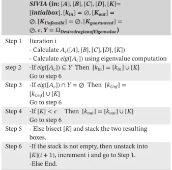
TABLE 1 The proposed recursive SIVIA-based algorithm to seek for a set of robust gains

SIVIA (in: [A], [B], [C], [D], [K]=

[intialbox], [kin] = ⊘, [Kout] = ⊘, [KUnfeasibl] = ⊘, [Kguaranteed] = ⊘, 𝜖, Y = ΩDesiredragionofEigenvalue)

Step 1 Iteration i

- Calculate Ac([A], [B], [C], [D], [K])

- Calculate eig([Ac])using eigenvalue computation step 2 -If eig([Ac]) ⊆ Y Then [kin] = [kin] ∪ [K]

Go to step 6

Step 3 -If eig([Ac]) ∩ Y = ⊘ Then [kUnf] = [kUnf] ∪ [K]

Go to step 6

Step 4 -If [K] < 𝜖 Then [kout] = [kout] ∪ [K] Go to step 6

Step 5 - Else bisect [K] and stack the two resulting boxes.

Step 6 -If the stack is not empty, then unstack into [K](i +1), increment i and go to Step 1. -Else End.

2. - taking into account the input constraints of the sys-tem in such a way that the control input will not exceed predefined amplitudes.

In this paper we propose to use the interval analysis to handle these two problems. For this matter, we propose to reformulate the problem as follows.

Problem: find the set of gains [K] of the closed-loop

system such that the following inclusions are satisfied: {

u∗_{([A], [B], [C], [D], [K]) ⊆ [U}

s, Us]

eig [Ac([A], [B], [C], [D], [K])] ⊆ ΩDesired region

(12) where [Ac]is the augmented closed-loop state matrix of the system (11), ΩDesired regionis the desired subregion of eigen-values, u*_{is the control input of the interval system. which}

will be detailed in the following subsection, and [Us, Us] are the lower and upper bounds of the control input mag-nitude that refers to the physical limitation of the actuator. They are constant and correspond to the maximal and minimal voltages that we can apply to the actuator.

3.3

Finding the set of gains that satisfy

the pole assignment specifications

In this subsection, the process of searching for a set of robust gains is transformed into a set inversion problem. Solving this latter problem permits finding the gains that assign the interval eigenvalue in the desired region.

A set inversion operation consists of searching the recip-rocal image called subpaving of a compact set. In our case, in order to solve this set inversion problem, we consider the Set Inversion Via Interval analysis (SIVIA) algorithm introduced in [38], which we propose to modify. We call the

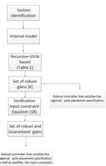
FIGURE 2 Recursive SIVIA-based algorithm with interval eigenvalues computation [Colour figure can be viewed at wileyonlinelibrary.com]

suggested modified algorithm the recursive SIVIA-based algorithm. In this recursive SIVIA-based algorithm, the aim is to approximate with subpaving the set solutions [K] that satisfy the inclusions (12).

The recursive SIVIA-based algorithm is outlined in Table 1 and depicted in Figure 2. To use this algorithm, we need to define an initial box [K0] that may contain

the solutions. Moreover, we should have as well the inter-val state-space matrices, the desired region of eigeninter-values (specifications), and the accuracy for the paving 𝜖. Since the closed-loop matrix of our system is non-symmetrical, we are obliged to use the Hla ˇd𝚤k formula [41] or the vertex approach [46] in the proposed SIVIA-based algorithm to calculate the interval eigenvalue. The proposed algorithm provides a complete information about the ranges of the feedback gains including: inner (solution), outer (unde-fined), and unfeasible (no solution) subpavings where all the sets' subpavings were initially empty. The inner solu-tion is the set of gains that ensure all the eigenvalues of the interval system are inside the desired region, whereas, the outer solution is the set of gains that guarantee that the inclusion condition is not satisfied. Finally, the unfea-sible solution is the border set where we do not have any conclusion.

3.4

Finding the set of gains that satisfy

the control input constraints

All physical systems should generally operate within bounds on the control input in order to avoid overpowering of the actuators because otherwise they may be damaged. It is therefore essential to consider these limitations, called

input constraints, during the controller design. In this sub-section we will convert the problem of input constrains into the inclusion problem by using the interval analysis technique [38]. Foremost, to streamline the notation let us start by redefining the closed-loop system (11) as descried by equations (3.4): (. x(t)_. 𝜉(t) ) = (A∗+ B∗K∗_C∗₎ ( x(t) 𝜉(t) ) + ( 0n×m Im×m ) r(t) . X(t) = Ac X(t) + Bc r(t) 𝑦(t) = (C∗+ D∗K∗_C∗₎ ( x(t) 𝜉(t) ) (13) Cc such that A∗₌ ( A 0n×p −C 0p×p ) ; B∗ = ( B − D ) ; C∗= ( C 0p×m 0m×n Im×m ) ; K∗ ₌(_k 𝑦 ki); D∗ = ( D 0p×m ) ;

The control input (10) can be reformulated as follows: (I + k𝑦D)u(t) = k𝑦Cc ( x(t) 𝜉(t) ) + 𝜉(t)Ki⇔ u(t) = (I + K∗_D∗₎−1_K∗(_Ct c Bc )t X(t) (14)

Since the closed-loop system will be asymptotically sta-ble for acceptasta-ble design, the maximum of the control input is observed when the derivative of the control input is equal to zero (i.e.,u = 0). Thus,.

. u = (I + K∗_D∗₎−1_K∗(_Ct c Bc )t. X(t) =0 ⇔ . u = (I + K∗_D∗₎−1_K∗(_Ct c Bc )t (AcX(t)∗+ Bcr(t)) = 0 (15)

For(I + K∗_D∗₎−1_K∗(_Ct

c Bc)t = 𝚵 and Ac are

non-singular matrices (i.e., 0 ∉ 𝜩, Ac), we have:

X∗_{(t) = −A}−1

c Bcr(t) (16)

The condition on non-singularity of Accan be easily sat-isfied using an eigenvalues assignment technique in which all the eigenvalues of the interval closed-loop matrix Accan be assigned to be strictly negative.

In certain applications of piezoelectric actuators, such as in micro/nano manipulation, the input force reference is always a step or a sequence of steps signal. Hence we assume r as constant reference or constant within an inter-val described by r ⊂ [r, r]. Actually piezoelectric actu-ators have a badly damped step response. Therefore in closed-loop, the input control is also oscillating in order to compensate for the system's oscillation. The idea here is to find the interval that embraces all possible values of the maximum input control when the reference trajectory takes a value inside the range [r, r]. The interval (the lower and upper bounds) of the input control can be calculated easily using the following interval computation.

With the help of equations (14) and (16) we derive the formula of the control input u*_{for the interval system (17):}

u∗_{= (I + K}∗_D∗₎−1_K∗(_Ct c Bc

)t

(−A−1c Bcr) (17) The interval formula of the input constraint (17) is used to convert the problem of inputs constraint to inclusion problem (18) that can be solved easily using the inversion algorithms as explained in the following subsection.

u∗_{([A], [B], [C], [D], [K]) ≡ [u, ̄u] ⊆ [U, ̄U] (18)}

3.5

Summary of the search of a robust

and guaranteed gains

In this subsection, the overall framework to find the set of gains that are robust and, at the same time that guaran-tee the input constraint is provided. The overall framework is depicted in Figure 3. The search for a set of robust and guaranteed gains is done in cascade as shown in the diagram of Figure 3. In practice, this can be done by adding the inclusion equation of the input constraint (18) in the second line of "step 2" of the recursive SIVIA-based algorithm (Table 1).

Furthermore, if one is only interested in finding the set of robust gains without input constraints, the searching pro-cess is stopped after the recursive SIVIA-based algorithm as shown in the diagram of Figure 3.

Remark. To search for the set of guaranteed gains

that satisfy the input constraints, we should first ver-ify the poles assignment specification to be sure that the closed-loop matrix Ac is non-singular as needed in (17). Therefore, the interval control input inclusion (18) is checked only inside the solution boxes [Kin] that

sat-FIGURE 3 Overall framework to obtain the set of robust and guaranteed gains [Colour figure can be viewed at

wileyonlinelibrary.com]

isfy the eigenvalues inclusion (12) where the closed-loop eigenvalues are certainly inside the desired region.

4

APPLICATION TO

PIEZOELECTRIC TUBE ACTUATORS

In this paper we apply the proposed modeling and con-trol technique to a piezoelectric tube actuator. An appli-cation of this actuator is the manipulation of miniatur-ized objects, see Figure 4. Such manipulation application (micromanipulation) requires micrometric precision and millisecond of response time. Unfortunately, the manip-ulator (the actuator) is often in an environment where the temperature could vary due to the surrounding exper-imental setup (camera lamp, devices,..) or to other natural sources [1]. The aim of this section is to use the proposed recursive SIVIA-based algorithm to find the robust and guaranteed controller gains to further control the manip-ulation force of the piezoelectric tube under these thermal variation conditions.

FIGURE 4 The use of piezoelectric tube actuator to manipulate a micro-object [Colour figure can be viewed at

wileyonlinelibrary.com]

4.1

Experimental setup

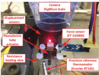
The experimental setup is represented in Figure 5. It is composed of a piezoelectric tube actuator (PT230.94), an optical displacement sensors (LC2420 from Keyence com-pany), a voltage amplifier (up to ±200V), a force sensor from femtotools-company (FT-S10000, max-10mN) and a computer with Matlab-Simulink for the implementation of the controller and for generating/acquiring the signals. A dSPACE-1103 acquisition board is used as an interface between the computer and the rest of the setup. The piezo-electric tube is made of lead-zirconate-titanate (PZT) mate-rial coated by one inner electrode (in silver) that serves as ground and four external electrodes (in copper-nickel alloy) for the electrical potentials. In addition, in order to stimulate an external variation of the ambient tempera-ture, we use a controllable heating resistance wire around the piezoelectric actuator as shown in Figure 5 and we use a precision reference thermometer (Eurolec RT161) to measure the temperature. In this experimental part, instead of manipulating micro-objects, we manipulate the cantilever of the force sensor as shown in Figure 5.

In order to inflect the tube along the X-axis or Y-axis, we apply a potential +U on one electrode and the oppo-site potential −U to the counterpart electrode as depicted in Figure 6 and . Furthermore, if we apply potentials with the same sign on the four electrodes we will cause a relative displacement on the Z-axis. In the terminal of the

piezo-FIGURE 5 Presentation of the experimental setup [Colour figure can be viewed at wileyonlinelibrary.com]

FIGURE 6 Structure and operation of the piezoelectric tube actuator [Colour figure can be viewed at wileyonlinelibrary.com] electric tube, we have placed a small cube with perpendic-ular and flat sides to serve as reflector for the displacement sensor.

4.2

Modeling of piezoelectric tube

actuator

During the experimental process we focus on the control of the manipulation force in one axis only (one degree of free-dom: 1-DoF). We will note Uxthe related applied voltage, and 𝜎xand Fxthe resulting deflection (displacement) and the applied force to the manipulated micro-object respec-tively in x direction. The relation between Ux, 𝜎xand Fx

can be expressed by the linear equation in (19), whereas the sensitivity of the actuator to the temperature variation will be modeled by parametric uncertainties bounded by intervals [1].

where sp and dp are the compliance and the piezoelec-tric constant respectively of the piezoelecpiezoelec-tric actuator. 𝛶 (s) represents the dynamics (with 𝛶 (0) = 1 ). A second order model has been chosen for the dynamic 𝛶 (s) as it includes the first resonance of the actuator and because of its simplicity [1].

The dynamics of the manipulated micro-object is rep-resented by a second order model reprep-resented by a spring-mass-damper system with an effective mass me, a viscous damping coefficient ceand a stiffness keas shown in Figure 6 and given by (20):

𝜎x= s0.Fx.Ψ(s) (20) where s0 is the micro-object compliance and 𝛹 (s) is its

dynamics part.

Finally, after replacing the deflection in (19) with that of (20), we obtain the following linear transfer between the voltage and the force:

Gxx=

Fx

Ux

= sp.𝛶 (s)

s0.Ψ(s) + sp.𝛶 (s)

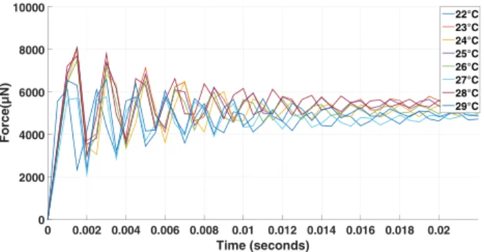
The previous model is a point model, that is, the eters are point. However, as we said before, these param-eters strongly depend on the temperature evolution. The model is therefore uncertain. We suggest here to transform this model into an uncertain model where the uncertain parameters are bounded by intervals. To do that, we apply a step voltage Uxof amplitude 10 V and capture its corre-sponding Fxunder several values of the ambient temper-ature varying between 22o_{C to 29}o_{C with an increment of} 1o_{C, as shown in Figure 7. It is worthy noting that the} ambi-ent temperature variation has an impact on the actuator as well as on the force sensor. For each step response taken at a given temperature Ti we use System Identification MatlabToolbox with Box-Jenkins method [49] to identify

Gxx(Ti). Note that for each temperature, the actuator is in contact with the object (the force sensor in this case). Finally, to derive the interval model [Gxx] of the piezo-electric actuator under temperature variation, we replace

FIGURE 7 Open-loop step response under several ambient temperatures [Colour figure can be viewed at

wileyonlinelibrary.com]

each parameter of Gxxby intervals as shown in (21). These intervals embrace all obtained values of each coefficient of

Gxx(Ti)under different temperature conditions: [Gxx] (s) = [ b0]s2+[b1]s +[b2] s2_{+ [a1] s + [a2]} (21) where [b0] = [346.5632, 423.5774] ; [a1] = [267.3284, 326.7348]; [b1] = [6.4855, 7.9268] ∗ 1e5; [a2] = [1.2419, 1.5180] ∗ 1e7; [b2] = [2.7233, 3.3286] ∗ 1e9;

In fact, there is a compromise between the widths of the intervals parameters and the chance to find the ade-quate feedback controller. For example, if we augment the range of the temperature variation, larger parameter inter-vals are obtained, which makes the search for adequate robust gains impossible.

It is worth noting that the interval model can also be obtained under only one temperature condition, for example 25o_{C. Then, the identified parameters under this} single temperature are considered as the center of the further interval parameters while the radius is imposed as 10%, see for instance [28,50]. This approach is sim-pler to implement than the above approach because the experimental characterization is carried out with one tem-perature only. However it does not guarantee that the real parameters with the various temperature will be bounded by the 10% that belong in this intervals radius.

Finally, from our interval transfer function model in (21), we derive the following state-space model in control canonical form: {. x(t) = Ax(t) + Bu(t) 𝑦(t) = Cx(t) + Du(t) (22) A = [ 0 1 −[a2] −[a1] ] ; B = [ 0 1 ] ; D = [b0] C =[[b2] − [a2][b0] [b1] − [a1][b0]]

4.3

Controller calculation

and experimental tests

The use of the interval model of the piezoelectric tube allows us to find a robust and guaranteed output-feedback controller that satisfies the desired performance under temperature variation. The following desired perfor-mances are adopted: negligible overshoot (1%) and with a settling time Ts ≤ 20ms. We found 𝜉 = 𝜂.𝜔n = 149.8 and 𝜃 = sin−1(𝜂) = 55, 7o, where 𝜂 and 𝜔nare the damp-ing ratio and natural pulsation respectively. Indeed, in micromanipulation and assembly applications, overshoots and oscillations are undesirable because they may cause micro/nano objects damage as well as instability in the tasks.

To calculate the set solutions [K] (with [K] = [[Ky] [Ki]]) we use the proposed recursive SIVIA-based algorithm described in Table 1. Foremost we choose an initial box [Ko] = [Ky] × [Ki] = [−10 × 10−1, 10 × 10−1] × [−6 × 10−3, 6 × 10−3_{]and an accuracy of paving 𝜖 = 10}−4_{. The choice of}

the initial box Ko is by trial and error. If there is no solu-tion within a given initial box, a different box is tested. Generally the initial box has not to be too small in order to be sure we have a large enough span. Meanwhile, a too large initial box results in time-consuming problem solv-ing. Regarding the input constraint Ux, it is supposed to be between [−20V, 20V], and the range of the input reference is r ⊂ [−10mN, 10mN].

After applying the proposed recursive SIVIA-based algorithm described, we obtain the subpaving as depicted in Figure 8. The red boxes correspond to the inner sub-pavings [Kin], that is, the set solutions [Ky]and [Ki]that satisfy the eigenvalue inclusion (12). The white boxes cor-respond to the subpavings [KUnfeasible]where the inclusion condition is guaranteed to be not satisfied. The yellow boxes refer to [Kout]where no decision on the inclusion is taken. The boxes in green correspond to the guaranteed set solution [Kguaranteed]in which both the inclusions condi-tion of the eigenvalue (12) and the input constraints (18) are verified.

Actually any choice inside the solutions [Kguaranteed]will ensure certainly the specified performances under temper-ature variation and input constraints. It could be possible to choose the optimal gains that ensure the best behaviors of the closed-loop among these solutions but this is out of the scope of this paper and is a future work.

We test now the obtained solutions in simulation and in experiments. For that we select arbitrary values of con-troller parameters from the set solutions in Figure 8: Ky= −0.1 × 10−3_{and K}

i = 0.3. The experimental and simula-tion step response for the closed-loop system are depicted in Figures 9 and 10.

FIGURE 8 Resulting subpaving of [Ky]and [Ki][Colour figure can be viewed at wileyonlinelibrary.com]

FIGURE 9 Step response of piezoelectric tube for the closed-loop system (Simulation using Matlab) [Colour figure can be viewed at wileyonlinelibrary.com]

FIGURE 10 Step response of piezoelectric tube for the closed-loop system (Experimental test) [Colour figure can be viewed at wileyonlinelibrary.com]

To perform the simulation, we take three different val-ues of the system matrices (A, B, C, D) inside the interval system ([A], [B], [C], [D]): the sup(), inf(), and mid() refer to the superior, inferior, and middle values of these inter-val matrices. Then the chosen controller above is applied to these three systems. Figure 9 displays the step response of the closed-loop system. It is clearly shown that the con-troller always ensures the desired performances (negligible overshoot (1%) and settling time less then 20ms) whenever the values of the matrices system (A, B, C, D) lie inside the interval system ([A], [B], [C], [D]).

Figure 10 represents the experimental results of the closed loop response acquired in various temperature con-ditions ( 22o_{C to 28}o_{C). The figure also shows that the} spec-ified performances (negligible overshoot (1%) and settling time less then 20ms) are also satisfied by the closed-loop for these various temperatures.

In order to verify the locations of the closed-loop eigen-values, we identify the closed-loop system of the experi-mental step responses given in Figure 10 ( 22o_{C to 28}o_C) using the Box-Jenkins method. We get second order mod-els with eigenvalues of negligible imaginary part and a real part within the interval of [−3500, −170]. It is evident that these obtained eigenvalues of the closed-loop system are included inside the desired region (Real(eig([Ac])) < −𝜉). Indeed, we have: [−3500, −170] ⊂] − ∞, −𝜉], with

FIGURE 11 Pursuit responses to series of steps for the closed-loop system [Colour figure can be viewed at wileyonlinelibrary.com]

We now test the tracking performance of the closed-loop system to follow a series of steps of input reference. The result is depicted in Figure 11 where it is clearly shown that the piezoelectric tube actuator tracks successfully the desired performances.

The simulation and the experimental results presented in Figures 9, 10 and 11 show that the proposed controller provided very good performances compared with works [23,28]. Furthermore, the controllers presented in [23,28] were only tested under a fixed ambient temperature. How-ever, in this paper the proposed controller was tested under temperature variation and input constraints.

5

CONCLUSIONS

In this paper, a simple algorithm to synthesize the robust and guaranteed controller to control the manipulation force of a piezoelectric tube actuator under tempera-ture variation and input constraint is proposed using output-feedback schema with integral compensator. The algorithm suggested to solve the problem is called a recur-sive SIVIA-based algorithm and is based on the combi-nation of the Set Inversion Via Interval Analysis (SIVIA) approach, intervals eigenvalues computation, and interval input inclusion techniques. Simulation tests and experi-mental applications on a piezoelectric tube actuator were carried out and demonstrated the efficiency of the pro-posed approach.

ORCID

Micky Rakotondrabe https://orcid.org/ 0000-0002-6413-7271

REFERENCES

1. M. Rakotondrabe et al., Smart materials-based actuators at the micro/nano-scale: Characterization, control and applications, Springer, Verlag, Berlin, 2013.

2. J.-W. Wu et al., Adaptive tilting angles to achieve high-precision scanning of a dual probes AFM, Asian J. Control 20 (2018), 1339–1351.

3. D. Habineza, M. Rakotondrabe, and Y. Le Gorrec, Characteriza-tion, modeling and h-inf control of n-dof piezoelectric actuators: Application to a 3-dof precise positioner, Asian J. Control 18 (2016), 1239–1258.

4. S. Rana, H. R. Pota, and I. R. Petersen, A survey of methods used to control piezoelectric tube scanners in high-speed AFM imaging, Asian J. Control 20 (2018), 1379–1399.

5. S. Devasia, E. Eleftheriou, and S. O. R. Moheimani, A survey of control issues in nanopositioning, IEEE Trans. Control Syst. Technol. 15 (2007), 802–823.

6. M. Rakotondrabe, Multivariable classical prandtl-ishlinskii hys-teresis modeling and compensation and sensorless control of a nonlinear 2-dof piezoactuator, Nonlinear Dyn 89 (2017), 481–499.

7. D. Niederberger, Smart Damping Materials Using shunt Control. Zürich, Switzerland: Eidgenossische Technische Hochschule ETH Zurich, Switzerland, 2005.

8. H. Aschemann, J. Minisini, and A. Rauh, Interval arithmetic techniques for the design of controllers for nonlinear dynamical systems with applications in mechatronics, J. Comput. Syst. Sci. Int. 49 (2010), no. 5, 5–16.

9. F. Ikhouane, V. Mañosa, and J. Rodellar, Adaptive control of a hysteretic structural system, Automatica 41 (2005), 225–231. 10. X. Tan and J. S. Baras, Adaptive identification and control of

hys-teresis in smart materials, IEEE Trans. Autom. Control 50 (2005), 827–839.

11. J. Yao and W. Deng, Active disturbance rejection adaptive control of uncertain nonlinear systems: Theory and application, Nonlin-ear Dyn. 89 (2017), 1611–1624.

12. F. Lydoire and P. Poignet, Nonlinear model predictive control via interval analysis, IEEE Conference on Decision and Control, Seville, Spain, 2005, pp. 3771–3776.

13. B. J. Kubica, Preliminary experiments with an interval model-predictive-control solver, Parallel Processing and Applied Mathematics, Springer, Cham, 2016, pp. 464–473.

14. H. Ma, J. Wu, and Z. Xiong, Pid saturation function sliding mode control for piezoelectric actuators, IEEE/ASME Advanced Intelligent Mechatronics, Besacon, France, 2014, pp. 257–262. 15. J. Li and L. Yang, Finite-time terminal sliding mode tracking

con-trol for piezoelectric actuators, Abs. and Appl. Anal. 2014 (2014), 9, 760937.

16. L. Yang, Z. Li, and G. Sun, Nano-positioning with sliding mode based control for piezoelectric actuators, International Confer-ence on Mechatronics and Control, Jinzhou, China, 2014, pp. 802–807.

17. S. F. Alem, I. Izadi, and F. Sheikholeslam, Adaptive sliding mode control of hysteresis in piezoelectric actuator, International Fed-eration of Automatic Control 50 (2017), 15574–15579.

18. S. H. Chung and E. Fung, Adaptive sliding mode control of piezoelectric tube actuator with hysteresis, creep and coupling effect, ASME International Mechanical Engineering Congress and Exposition, Vancouver, British Columbia, Canada, 2010, pp. 419–428.

19. Y. Li and Q. Xu, Adaptive sliding mode control with perturba-tion estimaperturba-tion and pid sliding surface for moperturba-tion tracking of a piezo-driven micromanipulator, IEEE Trans. Control Syst. Tech-nol. 18 (2010), 798–810.

20. M. Rakotondrabe, Y. Haddab, and P. Lutz, Quadrilateral modelling and robust control of a nonlinear piezoelectric cantilever, IEEE Trans. Control Syst. Technol. 3 (2009), 528–539.

21. S. Salapaka et al., High bandwidth nano-positioner: A robust control approach, Rev. Sci. Inst. 73 (2002), 3232–3241.

22. G. Schitter, A. Stemmer, and F. Allgower, Robust 2 dof-control of a piezoelectric tube scanner for high speed atomic force microscopy, American Control Conference, Denver, CO, USA, 2003, pp. 3720–3725.

23. S. Khadraoui, M. Rakotondrabe, and P. Lutz, Interval force/position modeling and control of a microgripper composed of two collaborative piezoelectric actuators and its automation, Int. J. Control Autom. Syst. 12 (2014), 358–371.

24. J. Bondia et al., Guaranteed tuning of pid controllers for para-metric uncertain systems, Conference on Decision and Control, Nassau, Bahamas, 2004, pp. 2948–2953.

25. V. L. Kharitonov, Asymptotic stability of an equilibrium position of a family of systems of differential equations, Differ. Equ. 14 (1978), 1483.

26. M. Rakotondrabe, Performances inclusion for stable interval sys-tems, American Control Conference, San Francisco, CA, USA, 2011, pp. 4367–4372.

27. S. Khadraoui, M. Rakotondrabe, and P. Lutz, Combining h-inf approach and interval tools to design a low order and robust controller for systems with parametric uncertainties: Appli-cation to piezoelectric actuators, Int. J. Control 85 (2012), 251–259.

28. S. Khadraoui, M. Rakotondrabe, and P. Lutz, Robust control for a class of interval model: Application to the force control of piezo-electric cantilevers, IEEE Conference on Decision and Control, Atlanta, GA, USA, 2010, pp. 4257–4262.

29. Y. Smagina and I. Brewer, Using interval arithmetic for robust state feedback design, Syst. Control Lett. 46 (2002), 187–194.

30. B. M. Patre and P. J. Deore, Robust state feedback for interval sys-tems: An interval analysis approach, Reliab. Comput. 14 (2010), 46–60.

31. M. L. M. Prado, A. Lordelo, and P. Ferreira, Robust pole assign-ment by state feedback control using interval analysis, World Congress, Prague, Czech, Brisbane, Australia, 2005, pp. 951–951. 32. K. Wei, Stabilization of linear time-invariant interval systems via constant state feedback control, IEEE Trans. Autom. Control 39 (1994), 22–32.

33. I. V. Dugarova. (1989). Application of interval analysis for the design of the control systems with uncertain parameters, Ph.D. Thesis, Tomsk State University, Russia.

34. L. Yu, Q. Han, and M. Sun, Optimal guaranteed cost control of linear uncertain systems with input constraints, Int. J. Control Autom. Syst. 3 (2005), 397–402.

35. L. Yu, An lmi approach to reliable guaranteed cost control of discrete-time systems with actuator failure, Appl. Math. Comput. 162 (2005), 1325–1331.

36. A. Al-Jiboory and G. Zhu, Robust input covariance constraint control for uncertain polytopic systems, Asian J. Control 18 (2015), no. 4, 1489–1500.

37. C. Clévy, M. Rakotondrabe, and N. Chaillet, Signal measure-ment and estimation techniques issues in the micro/cano world, Springer-Verlag, New York, 2011, page 978.

38. L. Jaulin, Applied interval analysis: With examples in param-eter and state estimation, robust control and robotics, Springer Science & Business Media, Berlin, London, UK, 2001.

39. A. Deif, The interval eigenvalue problem, J. Appl. Math. Mech. 71 (1991), no. 1, 61–64.

40. L. Kolev and S. Petrakieva, Assessing the stability of linear time-invariant continuous interval dynamic systems, IEEE Trans. Autom. Control 50 (2005), 393–397.

41. M. Hladík, Bounds on eigenvalues of real and complex interval matrices, Appl. Math. Comput. 219 (2013), 5584–5591. 42. G. Mayer, A unified approach to enclosure methods for eigenpairs,

J. Appl. Math. Mech. 74 (1994), 115–128.

43. H-S. Ahn, K. L. Moore, and Y. Chen, Monotonic convergent itera-tive learning controller design based on interval model conversion, IEEE Trans. Autom. Control 51 (2006), 366–371.

44. J. Rohn, A handbook of results on interval linear problems, Czech Academy of Sciences, 2005.

45. S. P. Bhattacharyya and L. H. Keel, Robust control: The para-metric approach, Advances in Control Education, Elsevier, Perg-amon, 1995, pp. 49–52.

46. M. T. Hussein, Assessing 3-d uncertain system stability by using matlab convex hull functions, Int. J. Adv. Comput. Sci. Appl. 2 (2011), 13–18.

47. V. Syrmos, C. Abdallah, P. Dorato, and K. Grigoriadis, Static output feedback a survey, Automatica 33 (1997), 125–137. 48. R. C. Dorf and R. H. Bishop, Modern control systems, Pearson,

London, Upper Saddle River, New Jersey, 1998.

49. L. Ljung, System identification toolbox: user's guide, Citeseer, Natick, MA USA, 1988.

50. M. Hammouche, P. Lutz, and M. Rakotondrabe, Robust feedback control for automated force/position control of piezoelectric tube based microgripper, IEEE Conference on Automation Science and Engineering, Xi'an, China, 2017, pp. 598–604.

AUTHOR BIOGRAPHIES

Mounir Hammouche

received the Engineer diploma in Control Engineering from the Ex-American Institute

of Boumerdes University

(Algeria) in 2012, Magister degrees in Automatic Control from the Polytech-nic School of Algiers (EMP) in 2014, and his master on the Technology of Information and Con-trol (ScTIC) at the university of Paris Est Créteil (UPEC) in 2015. He obtained the PhD degree from the Université Bourgogne Franche-Comté with research affiliation at the FEMTO-ST research institute in 2018. His research interests include the multi-input/multi-output (MIMO) modeling and robust control design for uncertain systems, control design using interval analysis, optimal con-trol, robust stability analysis and compensation of nonlinearities.

Philippe Lutz joined the

University of Franche-Comté, Besancon, as Professor in 2002. He was the head of the research group “Automated Systems for Micromanipula-tion and Micro-assembly” of the AS2M department of FEMTO-ST Institute from 2005 to 2011. He was the Director of the PhD graduate school of Engi-neering science and Microsystems with more than 400 PhD students from 2011 to February 2017, and he is currently the head of the Doctoral College. Since January 2017, he is the director of the AS2M Research department of FEMTO-ST. His research activities at FEMTO-ST are focused on the design and control of micro-nano systems, microgrippers, micro-nano robots, feeding systems and micro-nano manipulation, assembly stations, and Optimal design and control of piezoelectrically actuated com-pliant structures. P. Lutz received several awards of IEEE, authored over 90 refereed publications (50 in high standard journals), serves as associate editor for the IEEE Transaction on Automation Science and Engineering and as Technical Editor for the IEEE/ASME Transactions on Mechatronic, is mem-ber of several steering committees and is memmem-ber of the IEEE Robotics and Automation Society (RAS) Committee on Micro-Nano Robotics.

Micky Rakotondrabe

(S'05-M'07) received the HDR degree in control sys-tems from the Université de

Franche-Comté, Besan?on

France, in 2014. He has been an Assistant Professor in 2006-2007 and then Associate Professor in 2007-August 2019 with the

Université de Franche-Comté since 2007 with research affiliation at the FEMTO Institute, France. Since Sept 2019, he is Full Professor at the National School of Engineering (ENIT), a campus of the Toulouse INP, in Tarbes France.

Dr. Rakotondrabe is or was a member of the IEEE/RAS Technical Committee (TC) on Micro/Nano Robotics and Automation and of the IFAC TC on Mechatronics. He received several recognition prizes. In 2016, he was a recipient of the Big-On-Small Award during the IEEE MARSS International Conference. This award is to recog-nize a young professional (<40yo) with excellent performance and international visibility in the topics of mechatronics and automation for manip-ulation at small scales. In 2018, he is nominee for Distinguished Lecturer of Micro/Nano Robotics & Automation at the IEEE/RAS Society. He is or was an Associate Editor or a Guest Editor in pres-tigious journals related to Robotics, Automation and Mechatronics (IEEE/ASME Transactions on Mechatronics, IEEE Robotics and Automation Letters, IEEE Transactions on Electronics, IFAC Mechatronics, MDPI Actuators)

How to cite this article: Hammoiuche M, Lutz P, Rakotondrabe M. Robust and guaranteed output-feedback force control of piezoelectric actuator under temperature variation and input constraints. Asian J Control. 2020;22:2242–2253.