HAL Id: pastel-00797363
https://pastel.archives-ouvertes.fr/pastel-00797363
Submitted on 6 Mar 2013HAL is a multi-disciplinary open access archive for the deposit and dissemination of sci-entific research documents, whether they are pub-lished or not. The documents may come from teaching and research institutions in France or abroad, or from public or private research centers.
L’archive ouverte pluridisciplinaire HAL, est destinée au dépôt et à la diffusion de documents scientifiques de niveau recherche, publiés ou non, émanant des établissements d’enseignement et de recherche français ou étrangers, des laboratoires publics ou privés.
Propriétés effectives de matériaux architecturés
Justin Dirrenberger
To cite this version:
Justin Dirrenberger. Propriétés effectives de matériaux architecturés. Autre. Ecole Nationale Supérieure des Mines de Paris, 2012. Français. �NNT : 2012ENMP0045�. �pastel-00797363�
1
2
3
4
5
1234145467836391829836846489A2BCBD183École doctorale n
◦432: Sciences des Métiers de l’Ingénieur (SMI)
Doctorat ParisTech
T H È S E
pour obtenir le grade de docteur délivré par
l’École Nationale Supérieure des Mines de Paris
Spécialité “Science et Génie des Matériaux”
présentée et soutenue publiquement par
Justin DIRRENBERGER
le 10 décembre 2012
Propriétés effectives de matériaux architecturés
Effective properties of architectured materials
Directeurs de thèse: Samuel FOREST Dominique JEULIN
Jury
M. Yves BRÉCHET,Professeur, SIMAP, Grenoble-INP Président
M. Albrecht BERTRAM,Professeur, Otto-von-Guericke-Universität Magdeburg Rapporteur
M. Rémy DENDIEVEL,Professeur, SIMAP, Grenoble-INP Rapporteur
M. Michel BORNERT,Ingénieur en Chef des Ponts, Eaux et Forêts, Navier, École des Ponts-ParisTech Examinateur M. Pierre GILORMINI,Directeur de recherche, PIMM, Arts et Métiers-ParisTech / CNRS Examinateur
M. Marc THOMAS,Ingénieur de recherche, DMSM, ONERA Examinateur
M. François WILLOT,Chargé de recherche, CMM, MINES-ParisTech Invité
M. Samuel FOREST,Directeur de recherche, CdM, MINES-ParisTech / CNRS Directeur de thèse M. Dominique JEULIN,Directeur de recherche, CMM, MINES-ParisTech Directeur de thèse
Il ne s’agit plus de créer une belle œuvre, il faut savoir s’organiser une belle réclame. — Octave Mirbeau, Le Manuel du savoir-écrire (1889)
Remerciements / Acknowledgements
Quelle meilleure introduction pour un manuscrit de thèse que la périlleuse épreuve des remerciements ? S’ils sont à l’image du candidat, je pense volontiers qu’ils reflètent aussi le contenu de la thèse. Je me suis alors senti obligé de faire preuve de bon sens, d’audace et d’honnêteté intellectuelle, tout en essayant, tant bien que mal, d’éviter les lieux communs et le piège des émotions.
Mes premiers remerciements vont à mon directeur de thèse Samuel Forest, qui a bien voulu m’accorder sa confiance alors qu’il n’avait que peu d’éléments pour le convaincre. Ce serait un euphémisme de dire que j’ai beaucoup appris à ses côtés. Tous ceux qui ont l’honneur d’avoir été ses élèves savent quelle déférente affection ils éprouvent pour le Maître si bienveillant qui les a guidés. Maître scientifique, mais aussi source d’inspiration. Samuel, veuillez trouver ici un trop faible témoignage de toute la considération que je vous porte.
J’aimerais de la même façon exprimer ma gratitude toute particulière envers mon autre directeur de thèse, Dominique Jeulin, qui a su partager son enthousiasme et son savoir sans bornes au profane curieux que j’étais et qui m’a ainsi fait découvrir cette discipline passionnante qu’est la morphologie mathématique. Ce fût un honneur de préparer mon doctorat sous votre direction.
Je souhaiterais maintenant remercier les membres de mon jury d’avoir accepter de se pencher sur mes travaux, en commençant par les rapporteurs. Ich danke Prof. Albrecht Bertram für das akribische Studium meiner Doktorarbeit und für seine einschlägigen Bemerkungen. Zudem danke ich ihm dafür, dass er mir durch sein Seminar an der École des Mines eine neue Sichtweise auf die Kontinuumsmechanik aufgezeigt hat. Un grand merci à Rémy Dendievel pour avoir accepté de rapporter sur ce travail à la dernière minute, et pour avoir constamment enrichi ma réflexion au cours de ces trois dernières années.
J’adresse mes plus sincères remerciements à Yves Bréchet pour avoir bien voulu présider mon jury de thèse. Je garderai un souvenir intense de nos discussions animées à propos du marquis de Condorcet ou de la bielle architecturée et autres moutons pentapodes.
Remerciements / Acknowledgements
Sans la contribution discrète de Michel Bornert, je n’aurais peut-être jamais entrepris une thèse en mécanique des matériaux. En effet, c’est en suivant son cours de master que je me suis intéressé à la question. Nos chemins se sont croisés à maintes reprises ces quatre dernières années, j’espère que ce n’est qu’un début ; je vous remercie d’avoir bien voulu juger mon travail. Merci à Pierre Gilormini de m’avoir fait l’honneur d’apporter, avec l’art et la manière, les précisions nécessaires à mon manuscrit lors de la soutenance. Je souhaiterais remercier chaleureusement Marc Thomas d’avoir participé en tant qu’examinateur à mon jury de thèse, merci également à François Willot d’y avoir pris part.
Une thèse se résume parfois à trois années de frustration face à une expérience infructueuse ou à taper des lignes de code vertes sur un écran noir. Dans mon cas ça a aussi été l’occasion de participer à un certain nombre de réunions d’avancement du projet ANR MANSART et de côtoyer des gens avec qui j’ai apprécié travailler. Je remercie Marc Thomas et Yves Bréchet d’avoir si bien mené la barque du projet MANSART et fait émerger un environnement que je qualifierais d’exceptionnel pour les doctorants. Sans m’étendre davantage et sans ordre particulier, merci à Magali Dugué, Amélie Kolopp, Marion Amiot, Loïc Courtois, Pierre Leite, Christophe Bouvet, Dominique Poquillon, Valia Fascio, Yannick Girard, Sophie Gourdet, Cécile Davoine, Frank Simon, Eric Maire, Michel Perez, Marc Fivel, Pierrick Péchambert, Dominique Bissières, Anne Perwuelz, Maryline Lewandowski et Sjoerd van der Veen.
Ce travail a été préparé principalement au Centre des Matériaux à Evry, dont j’aimerais remercier les 3 directeurs successifs, Esteban Busso, Yves Bienvenu et Jacques Besson, pour m’avoir accueilli et fourni dans un environnement de travail lui aussi exceptionnel. Je souhaiterais remercier l’ensemble des membres du CdM pour leur convivialité et plus spécifiquement Olivier et Grégory pour le support informatique indispensable, Odile pour les références bibliographiques improbables, Véronique pour le support logistique, Liliane et Konaly pour la pré-soutenance. J’ai eu la chance de collaborer avec plusieurs équipes au CdM, merci donc à l’équipe SIP, notamment Jean-Dominique Bartout et Christophe Colin, merci à l’équipe VAL, notamment Djamel Missoum-Benziane pour ses Zébulonneries et Nikolay Osipov pour le maillage, et enfin un grand merci à l’équipe COCAS et ses membres distingués, Georges Cailletaud, David Ryckelynck et Matthieu Mazière. Merci à Anne-Françoise Gourgues-Lorenzon pour m’avoir incité à aller regarder la microstructure de mes échantillons. Merci à Jérôme Crépin pour ses précieux conseils que j’ai tenté de mettre en application tant bien que mal. Merci à Franck N’Guyen pour son aide en Matlab et en C++.
Merci aux camarades du bureau B127, Nicolas, Damien, Bahram, Édouard, Ozgur, Victor, Aurélien et Mouhcine. Merci aussi à Meriem, Anthony, Antonin, Xu, Olivier, Manu, Pierre, Duy, Laure-Line, Morgane, Arina, Prajwal, Arthur, Konstantin, Charlotte, Rémi, Mamane, Christophe, Guillaume, Julian, Laurent, Flora, Mélanie, Antoine, Jia, Judith, Philippe et Francesco au CdM, ainsi que Noémie, Alexandre et Dominique à l’ONERA. J’ai aussi eu la chance d’être accueilli par l’équipe du Centre de Morphologie Mathématique à Fontainebleau, je tiens à remercier tout particulièrement Charles Peyrega, Julie Escoda, Matthieu Faessel et Hellen Altendorf. Merci aussi aux compagnons de route des matériaux architecturés, Olivier Bouaziz, Laurent Laszczyk, Arthur Lebée, Sébastien Turcaud, Lorenzo Guiducci et John Dunlop. Je remercie chaleureusement Felix Fritzen pour ses passages, toujours enrichissants, au CdM.
Remerciements / Acknowledgements
J’aimerais aussi profiter de l’occasion pour remercier Clotilde Berdin de l’Université Paris-Sud pour m’avoir permis d’enseigner pendant ma thèse.
Je tiens aussi à remercier spécialement André Pineau pour nos nombreuses discussions à bâtons rompus sur l’industrie, la recherche, l’histoire des idées et, bien sûr, les aciers inoxydables, en espérant qu’il ne m’en veuille pas trop de partir étudier les bétons en Angleterre...
D’une manière générale, je tiens à remercier toutes les personnes qui m’ont accordé leur confiance ou qui m’ont laissé ma chance au cours de mes études, il aura fallu un invraisemblable concours de circonstances pour que je termine ce chapitre de ma vie. Sans nommer les acteurs de cette aventure, je leur rends ici hommage.
Merci à mes parents, à Lucas et à Matthieu pour leur soutien indéfectible depuis 1985.
Pour finir, mes sentiments les plus profonds et ma gratitude la plus sincère sont adressés à la best partner in crime ever, Flo. La réalisation de ce projet n’aurait jamais été possible sans ta patience et ton soutien continu depuis toutes ces années. Ta belle âme m’inspire quotidiennement, j’espère que tu voudras bien assumer cette responsabilité encore quelques décennies.
Paris, le 23 janvier 2013 Justin Dirrenberger
Abstract
Architectured materials bring new possibilities in terms of structural and functional properties, filling gaps and pushing the boundaries of Ashby’s materials maps. The term "architectured materials" encompasses any microstructure designed in a thoughtful fashion, so that some of its materials properties have been improved. There are many examples: particulate and fibrous composites, foams, sandwich structures, woven materials, lattice structures, etc. One engineering challenge is to predict the effective properties of such materials. In this work, two types of microstructures are considered: periodic auxetic lattices and stochastic fibrous networks. Auxet-ics are materials with negative Poisson’s ratio that have been engineered since the mid-1980s. Such materials have been expected to present enhanced mechanical properties such as shear modulus or indentation resistance. The stochastic fibrous networks considered in this work is made of 3D infinite interpenetrating fibers that are randomly distributed and oriented. This case of random structure is challenging regarding the determination of a volume element size that is statistically representative. For both materials, computational homogenization using finite ele-ment analysis is impleele-mented in order to estimate the effective thermal and mechanical properties. Keywords: Computational homogenization, Representative Volume Element, Auxetics, Ran-dom fibrous networks, Effective properties
Résumé
Les matériaux architecturés font émerger de nouvelles possibilités en termes de propriétés struc-turales et fonctionnelles, repoussant ainsi les limites des cartes d’Ashby. Le terme "matériaux architecturés" inclus toute microstructure conçue de façon astucieuse, de sorte que certaines de ses propriétés soient optimisées. Les exemples sont nombreux : composites fibreux et particulaires, matériaux cellulaires, structures sandwiches, matériaux tissés, structures treillis, etc. Un enjeu de taille pour l’emploi de tels matériaux est la prédiction de leurs propriétés effectives. Dans ce travail, deux types de microstructures sont considérés : des structures auxétiques périodiques et des milieux fibreux aléatoires. Les auxétiques sont des matériaux apparus au milieu des années 1980, présentant un coefficient de Poisson négatif. On attend des auxétiques qu’ils présentent des propriétés mécaniques améliorées, comme le module de cisaillement ou la résistance à l’indentation. Les milieux fibreux aléatoires considérés dans ce travail sont constitués de fibres 3D infinies interpénétrantes aléatoirement distribuées et orientées. Ce type de structure aléatoire est très défavorable à la détermination d’une taille de volume élémentaire statistiquement repré-sentatif. Pour les deux types de matériaux, l’homogénéisation numérique à l’aide de la méthode des éléments finis est implémentée dans le but d’estimer les propriétés thermiques et mécaniques effectives.
Mots-clés : Homogénéisation numérique, Volume élémentaire représentatif, Auxétiques, Mi-lieux fibreux stochastiques, Propriétés effectives
Contents
Remerciements / Acknowledgements iii
Abstract (English/Français) vii
List of notations xv
Introduction 1
0 Architectured Materials 3
0.1 A new class of materials . . . 3
0.2 The MANSART project . . . 6
0.3 The present study . . . 7
0.4 From local heterogeneity to global response of materials . . . 8
0.5 Summary . . . 8
I Introduction to homogenization 9 1 Preliminary concepts 11 1.1 Constitutive thermal behavior . . . 11
1.2 Principles for mechanical modeling . . . 12
1.3 Constitutive mechanical behavior. . . 12
1.3.1 Linear elasticity . . . 12
1.3.2 Elastoplasticity . . . 14
1.4 Additivity . . . 16
2 Homogenization 17 2.1 Representative volume element . . . 17
2.2 Averaging relations. . . 19
2.2.1 Averaging thermal fields . . . 19
2.2.2 Averaging mechanical fields . . . 20
2.3 Boundary conditions . . . 21
Contents
2.3.2 Mechanical behavior . . . 22
2.3.3 Hill–Mandel condition . . . 24
2.4 Effective properties vs. apparent properties . . . 25
2.4.1 Linear conductivity . . . 25
2.4.2 Linear elasticity . . . 26
2.5 Some boundary value problems for the estimation of isotropic effective properties 29 2.5.1 Thermal properties . . . 29
2.5.2 Elastic properties . . . 30
3 Analytical estimates and bounds 33 3.1 Analytical estimates for thermal properties . . . 33
3.1.1 Maxwell Garnett’s estimate . . . 33
3.1.2 Bruggeman’s self-consistent model . . . 34
3.2 Analytical bounds for thermal properties . . . 35
3.2.1 Bounds of order 0 . . . 35
3.2.2 Bounds of order 1 . . . 35
3.2.3 Bounds of order 2 . . . 36
3.2.4 Bounds of order 3 . . . 37
3.2.5 Bounds of order 4 . . . 37
3.3 Analytical estimates for elastic properties . . . 38
3.3.1 Einstein’s estimate . . . 38
3.3.2 Eshelby’s model . . . 38
3.3.3 Self-consistent scheme . . . 41
3.4 Analytical bounds for elastic properties . . . 43
3.4.1 Bounds of order 0 . . . 43 3.4.2 Bounds of order 1 . . . 43 3.4.3 Bounds of order 2 . . . 44 3.4.4 Bounds of order 3 . . . 46 3.4.5 Bounds of order 4 . . . 47 4 Computational homogenization 51 4.1 Computational homogenization using the finite element method . . . 51
4.1.1 FE formulation of the principle of virtual work . . . 52
4.1.2 Application to linear elasticity . . . 53
4.1.3 The element DOF method with prescribed macroscopic strain. . . 54
4.2 Statistical approach for determining a RVE size . . . 56
4.2.1 Ergodicity hypothesis . . . 56
4.2.2 Stationarity hypothesis . . . 57
4.2.3 Statistical homogeneity hypothesis . . . 57
4.2.4 RVE size determination for media with finite integral range . . . 57
4.2.5 Generalization of the statistical approach to microstructures with non-finite integral range . . . 60 xii
Contents
II Application to periodic media 65
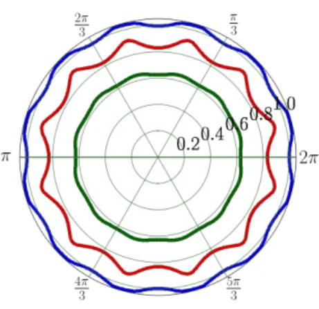
5 Auxetics 67 5.1 Introduction to auxetics . . . 67 5.2 Computational homogenization . . . 69 5.3 Microstructures considered . . . 70 5.3.1 Hexachiral lattice . . . 70 5.3.2 Anti-tetrachiral lattice. . . 71 5.3.3 Rotachiral lattice . . . 72 5.3.4 Honeycomb lattice . . . 72
5.4 Effective elastic properties. . . 73
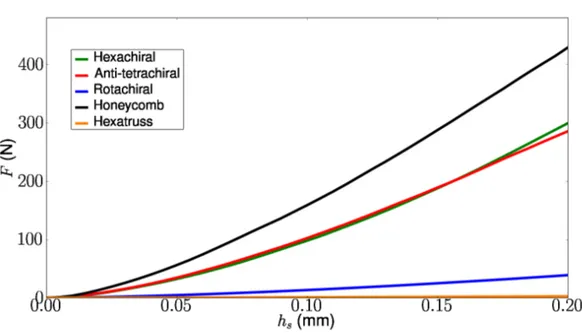
5.4.1 Hexachiral lattice . . . 75 5.4.2 Anti-tetrachiral lattice. . . 76 5.4.3 Rotachiral lattice . . . 78 5.4.4 Honeycomb lattice . . . 80 5.4.5 Discussion . . . 80 5.5 Extension to elastoplasticity. . . 82
5.5.1 Constitutive model considered . . . 82
5.5.2 Comparison with the honeycomb lattice . . . 86
5.5.3 Macroscopic modeling . . . 87
5.5.4 Simulation and identification. . . 90
5.5.5 Discussion . . . 92
5.6 3D auxetic microstructure: the hexatruss lattice. . . 92
5.7 Structural applications of auxetics . . . 94
5.7.1 Spherical indentation: loading case 1 . . . 95
5.7.2 Spherical indentation: loading case 2 . . . 96
5.7.3 Cylindrical indentation . . . 96
5.8 Experimental characterization of auxetics . . . 102
5.9 Conclusions and prospects. . . 102
III Application to random media 107 6 Poisson fibers 109 6.1 Microstructural model . . . 111
6.1.1 Poisson point process . . . 111
6.1.2 Linear Poisson varieties . . . 112
6.1.3 Boolean random sets . . . 112
6.1.4 Generation of Poisson fiber virtual models . . . 113
6.1.5 Discretization of microstructural models . . . 114
6.1.6 Parameters of the simulation . . . 116
6.1.7 Computational strategy . . . 116
Contents 6.2.1 Thermal properties . . . 121 6.2.2 Mechanical properties . . . 128 6.3 Results . . . 140 6.3.1 Morphological properties. . . 140 6.3.2 Thermal properties . . . 141 6.3.3 Elastic properties . . . 143 6.4 Discussion. . . 143 6.4.1 Morphological isotropy. . . 145 6.4.2 Elastic isotropy . . . 146
6.4.3 Thermal and mechanical fields. . . 149
6.5 Determination of the statistical RVE size . . . 151
6.5.1 Variance from simulation. . . 151
6.5.2 Results . . . 151
6.6 Conclusion . . . 155
IV Conclusions & Outlook 159 V Appendices 169 A Finite element method for periodic homogenization 171 A.1 Case study #1: fiber-reinforced composite material. . . 171
A.1.1 The MPC_periodic method . . . 172
A.1.2 The element DOF method with prescribed macroscopic strain. . . 175
A.1.3 The element DOF method with prescribed macroscopic stress. . . 177
A.2 Case study #2: 3D grid. . . 180
A.2.1 The MPC_periodic method . . . 181
A.2.2 The element DOF method with prescribed macroscopic strain. . . 182
A.2.3 The element DOF method with prescribed macroscopic stress. . . 183
B Basics of mathematical morphology 189 B.1 Characterization of random structures . . . 190
B.1.1 Minkowski functionals . . . 190
B.1.2 Basic operations of mathematical morphology. . . 190
B.1.3 Steiner formulae. . . 191
B.1.4 Covariance . . . 192
B.2 Models of random structures . . . 193
B.2.1 Choquet capacity . . . 193
B.2.2 Poisson point process . . . 194
B.2.3 Poisson linear varieties . . . 195
B.2.4 Boolean model. . . 197
B.2.5 Boolean random varieties . . . 198 xiv
Contents
B.2.6 Poisson fibres . . . 199
C Experimental characterization of auxetics 201
C.1 Microstructural characterization . . . 201
C.2 Macroscopic mechanical testing . . . 203
C.3 X-ray microtomography . . . 204
D Simulation results for Poisson fibers 209
References 214
Index 229
List of Notations
Tensors, tensor algebra and operators
x 0th-order tensor (scalar)
x orxi 1st-order tensor (vector)
x∼ orxi j 2nd-order tensor x ≈ orxi j kl 4 th-order tensor I ∼ orIi j 2
nd-order identity tensor
I
≈ orIi j kl 4
th-order identity tensor
ei Basis vector x = a · b x = aibi x = a∼· b xi= ai jbj x∼= a∼· b∼ xi j= ai kbk j x = a∼: b∼ x = ai jbi j x∼= a≈: b∼ xi j= ai j klbkl x = a≈:: b ≈ x = ai j klbi j kl x∼= a ⊗ b xi j= ajbj x∼= a ⊗ b =s 1 2 ³ a ⊗ b +¡a ⊗ b¢T´ x(i j )= 1 2 ¡ aibj+ ajbi ¢ x ≈= a∼⊗ b∼ xi j kl= ai jbkl δi j Kroneckersymbol ¯
¯¯¯x¯¯¯¯ Euclidean norm of a vector I1(x∼)orTr x∼orxi i 1stinvariant of a tensor (trace)
I2(x∼)or 1 2 ³¡ Tr x∼¢2− Tr¡x∼2¢´ 2ndinvariant of a tensor I3(x∼)orDet x∼ 3
rdinvariant of a tensor (determinant)
x∼−1 Inverse of an invertible tensor
x∼T Transpose of a tensor
Div x∼ or∇ · x∼ orxi j , j Divergence of a tensor
∇x∼ or∇ ⊗ x∼ Gradient of a tensor
˙
x∼=d x∼
d t Time derivative of a tensor
J
≈ Spherical projector for2
nd-order symmetric tensors
Contents
Thermal and mechanical tensors
Dt h Thermal dissipation rate density
q orqi Heat flux vector
T Temperature
∇T orT,i Temperature gradient
λ∼ orλi j Thermal conductivity tensor
ρ
∼ orρi j Thermal resistivity tensor
Eel Elastic strain energy density
σ∼ orσi j Cauchystress tensor
ε∼orεi j Engineering strain tensor
c
≈ orci j kl orcI J Elastic moduli tensor
s
≈orsi j l korsI J Compliance tensor
σ∼sph=1 3 ¡
Tr σ∼¢I∼ Spherical stress tensor σ∼dev= σ∼− σ∼
sph Deviatoric stress tensor
X∼ Kinematic hardening tensor
H ≈ Hilltensor v Velocity field u Displacement field f Body forces F Surface forces
Pint Power of internal forces
Pext Power of external forces
τ∼ Polarization stress tensor
S
≈
0 Eshelbyinteraction tensor
P
≈
0 Hillinteraction tensor
C
≈
⋆ Hillinfluence tensor
E Young’s modulus
µ Shear modulus
k Bulk modulus
ν Poisson’s ratio
Finite element notations
[x] n-dimensional matrix
{x} Column-vector
[N ] Shape function matrix
[B ] Deformation operator
[K ] Stiffness matrix
Contents
Mathematical morphology
A Random closed set
Ac Complementary set ofA
ˇ
A = {−x, x ∈ A} Transposed set ofA B (r ) Closed ball with radiusr
K Compact set P Probability of an event p = P {x ∈ A} Probability ofxto be in A q = P©x ∈ Acª= 1 − p Probability ofxto be in Ac C (h) = P {x ∈ A, x + h ∈ A} CovarianceC (h) Q(h) = P©x ∈ Ac, x + h ∈ Acª CovarianceQ(h) T (K ) = P {K ∩ A 6= ;} = 1 −Q (K ) Choquet’s capacity
W2(x, x+ h) 2ndorder central correlation function
A ⊕ ˇK Dilation by a compactK A ⊖ ˇK Erosion by a compactK AK = A ⊖ ˇK ⊕ K Opening by a compactK AK = A ⊕ ˇK ⊖ K Closing by a compactK µ (A) Measure ofA µn Lebesguemeasure inRn
θk Radonmeasure on locally compact topological spaces
N (A) Integral of total curvature or connectivity ofA
M(A) Integral of mean curvature ofA
L(A) Perimeter ofAinR2 A(A) Area ofAinR2 S (A) Area ofAinR3 V (A) Volume ofA SS Surface fraction VV Volume fraction
Z (x) Random function or physical property E {Z (x)} Mathematical expectation ofZ (x)
D2Z Variance ofZ (x)
DZ Standard deviation ofZ (x)
Z (V ) Average value overV ofZ (x)
An Integral range of dimensionn
ǫabs Absolute error
ǫrel Relative error
θ Intensity of a Poisson process
ω Random orientation inRn
Vk(ω) Poissonvariety with intensityθ (ω)
A′ Primary grain of a Boolean model
K (h) = µn
¡
Part
0
Architectured Materials
Accident is design And design is accident In a cloud of unknowing. — T. S. Eliot, The Family Reunion (1939)
0.1
A new class of materials
Architectured materials are a rising class of materials that bring new possibilities in terms of functional properties, filling the gaps and pushing the limits of Ashby’s materials per-formance maps [Ashby, 1999], as shown on Figure 1 [Ashby, 2013]. The term architec-tured materialsencompasses any microstructure designed in a thoughtful fashion, that some of its materials properties have been improved in comparison to those of its constituents
[Ashby and Bréchet, 2003, Ashby, 2013, Bréchet and Embury, 2013]. There are many
exam-ples: particulate and fibrous composites, foams, sandwich structures, woven materials, lattice structures, etc. Most of them are shown on Figure2, also taken from [Ashby, 2013]. One can play on many parameters to obtain architectured materials, but all of them are related either to the microstructure or the geometry. Parameters related to the microstructure can be optimised for specific needs using a materials-by-design approach, which has been thoroughly developed by chemists, materials scientists and metallurgists. For instance, it is well-known among met-allurgists that mechanically decreasing the average grain size of an alloy, as well as increasing the dislocation density, results in a higher yield strength. Stronger polymers can be engineered by changing interchain bounds or by optimizing the chain design. These improvements are intrinsically related to the synthesis and processing of materials and are therefore due to micro-and nanoscale phenomena, taking place at a scale ranging from 1 nm to 10 µm. This scale is below the scope of this work but has been extensively studied in the literature, see for instance
Chapter 0. Architectured Materials
Figure 1: Ashby’s material map for Young’s modulus vs. density, from [Ashby, 2013]
the key technological lock for the development of architectured materials, nevertheless progress is made every day to overcome this, as it was done in [Schaedler et al., 2011] by combining several processing techniques in order to fabricate ultralight metallic microlattice materials. From a macroscopic viewpoint, parameters related to the geometry have mainly been the responsibility of structural and civil engineers for centuries: to efficiently distribute materials within structures. An obvious example would be the many different strategies available for building bridges. Figure3, taken from [Ashby and Bréchet, 2003], illustrates the basic strength of materials fact that one can optimize bending stiffness by modifying the geometry of the component, keeping the lineic mass (for beams) or surfacic mass (for plates) unchanged. On the other hand, one might need a lower flexural strength for the same lineic and surfacic masses. This can be achieved with stranded structures, as shown on Figure 4, also taken from [Ashby and Bréchet, 2003]. Architectured materials thus lie between the microscale and the macroscale. This class of materials involves geometrically engineered distributions of microstructural phases at a scale comparable to the scale of the component, thus calling for new models in order to determine the effective properties of materials. One aim of the present work is to provide such models, in the case of mechanical and thermal properties.
0.1. A new class of materials
Figure 2: Examples of architectured materials, from [Ashby, 2013]
Figure 3: Shape as a parameter for increasing sectional bending stiffness, from
Chapter 0. Architectured Materials
Figure 4: Shape as a parameter for decreasing sectional bending stiffness, from
[Ashby and Bréchet, 2003]
0.2
The MANSART project
The MANSART (for MAtériaux saNdwicheS ARchiTecturés, or ARchiTectured saNdwicheS MAterials) project aims at exploring new tools and approaches to develop such materials. The project is mostly funded by the French Agence Nationale pour la Recherche (ANR). Starting from January 2009, the project ran for 4 years, gathering 5 industrial (Airbus, EADS-IW, ON-ERA, Ateca, SMCI) and 6 academic partners (CdM/MINES-ParisTech, MATEIS/INSA Lyon, SIMAP/Grenoble-INP, GEMTEX/ENSAIT, ICA/ISAE, CIRIMAT/ENSIACET). It is subsequent to the previous ANR project MAPO (MAtériaux POreux) and CNRS project MAM (Matéri-aux Architecturés Multifonctionnels). The applications considered in the MANSART project are mainly related to crashworthiness and mechanical properties at mid-range temperatures (ca. 300◦C ). The following architectured materials were considered to fulfill industrial require-ments: entangled monofilament of perlitic steel (PhD work of Loïc Courtois at MATEIS/INSA Lyon [Courtois et al., 2011]), sandwich composite structures (PhD work of Amélie Kolopp at ICA/ISAE [Kolopp et al., 2011]), woven and non-woven textile composites (PhD work of Mar-ion Amiotat GEMTEX/ENSAIT [Lewandowski et al., 2012]), segmented interlocking structures (PhD work of Magali Dugué at SIMAP/Grenoble-INP) and materials with negative Poisson’s ratio (this work). Moreover, optimization of sandwich structures was also investigated (PhD work of Pierre Leite at ONERA [Leite et al., 2012b,Leite et al., 2012a]), as well as homogenization methods for predicting the effective properties of architectured materials (this work).
0.3. The present study
0.3
The present study
This work is part of the MANSART project and was funded entirely by ANR. While most of the work was conducted at the Centre des Matériaux1, which is a mixed research unit between MINES-ParisTech and CNRS located in Evry, some of it, especially most of the computational microstructural modeling, was done at the Centre de Morphologie Mathématique2of MINES-ParisTech in Fontainebleau.
The study is part of MANSART, with a focus on computational modeling as well as rapid prototyping of architectured materials. As a matter of fact, one engineering challenge is to predict the effective properties of such materials; numerical homogenization using finite element analysis is a powerful tool to do so. A challenging candidate material was imagined for assessing the applicability of such methods to architectured materials: stochastic random networks made of infinite fibers, more specifically Poissonian fibrous networks. The determination of the effective properties of Poisson fibers is not trivial, as it will be presented in Part III of this manuscript. The random fibrous media considered in this work do not exist per se, but their microstructure can be modeled computationally. The generation of such virtual specimens relies on a tridimensional Poisson point implantation process. Due to the long-range correlation induced by the model of random structures chosen, the size of the representative volume element is a prioriunknown. One goal of this work was then to evaluate this size using numerical simulation. However, periodization of these microstructures is generally impossible, making the periodic homogenization tools ineffective. Very large virtual samples computations have to be performed in order to compute their representative volume element sizes a posteriori based on statistical arguments and finally predict their effective mechanical and thermal properties.
Another type of material was considered soon after we started the project: auxetics. Auxetic materials are a type of architectured materials exhibiting a negative Poisson’s ratio. They could present interesting advantages for both functional and structural applications in the future. They are presented in detail in Section 5.1. Auxetics considered in this work are halfway between lattice structures and foams. We worked on periodic structures, making their homogenization straightforward. A whole design-simulation-processing-characterization chain was developed for auxetics, making it possible for us to study numerically and experimentally auxetics from the literature, but also to develop new auxetic microstructures, using computer-aided design, results from homogenization, rapid prototyping with selective laser melting and mechanical testing. The results for auxetics are presented in PartII. By the means of homogenization technique coupled with finite elements, we were able to investigate anisotropy for both linear elasticity and elastoplasticity. Macroscopic modeling was performed and the simulation of indentation experiments was done using these models.
This work is aiming at helping us developing new architectured materials by understanding the underlying processes taking place in auxetic periodic lattices structures and stochastic random
1http://www.mat.ensmp.fr/ 2http://cmm.ensmp.fr/
Chapter 0. Architectured Materials
fibrous media. Rapid prototyping using selective laser melting allows us to be creative in terms of microstructural design. Our intention is also to demonstrate the ability of the computational homogenization using finite element analysis to be a powerful tool for designing, modeling and simulating future architectured materials.
0.4
From local heterogeneity to global response of materials
Materials science comes from the following fact: microstructural heterogeneities play a critical role in the macroscopic behavior of a material. Constitutive modeling, thanks to an interaction between experiments and simulation, is usually able to describe the response of most materials in use. Such phenomenological models, including little to no information about the microstructure, cannot necessarily account for local fluctuation of properties. In that case, the material is considered as a homogeneous medium. Studying the behavior of heterogeneous materials involves developing enriched models including morphological information about the microstructure. These models should be robust enough to predict effective properties depending on statistical data (volume fraction,n-point correlation function, etc.) and the physical nature of each phase
or constituent. As a matter of fact, advanced models are often restricted to a limited variety of materials. For instance, the behavior of a polycrystalline material without any particular texture, a multi-layered composite structure and a metallic ceramic exhibiting a composition gradient cannot be modeled using the same assumptions. Although isotropic and anisotropic polycrystalline metals have been extensively studied by the means of analytical and computational tools, architectured materials bring up new challenges regarding the determination of effective properties. The core purpose of this work is to meet up these challenges by adapting existing homogenization methods to architectured materials.
0.5
Summary
In this work, we intend on bringing up answers for the following questions:
• How to determine the effective properties of architectured materials? • How could we adapt existing computational tools for this purpose? • Can rapid prototyping be useful to develop architectured materials? • What can be expected from negative Poisson’s ratio materials? • How could we assess the representativity of elementary volumes?
Those questions will be covered in the discussion taking place in PartIV.
Part I
1
Preliminary concepts
Experience is simply the name we give our mistakes. — Oscar Wilde, Lady Windermere’s Fan (1892)
Our scientific goal is the prediction of the mechanical and thermal effective properties for architectured materials using computational homogenization. This first part aims at introducing homogenization methods and summarizing some approaches in this field, either analytical or computational.
Several considerations are necessary for implementing a homogenization scheme. They are presented hereafter.
A few assumptions have to be made regarding the physics of the materials studied in this work. They concern the constitutive thermal and mechanical behavior, as well as some related principles.
1.1
Constitutive thermal behavior
Thermal properties of architectured materials are studied in this work. We assume that heat trans-fer takes place within the material to be defined locally according to Fourier’s law [Fourier, 1822]:
Chapter 1. Preliminary concepts
withq heat flux density vector,λ∼ second-order symmetric tensor of thermal conductivity, and∇T
temperature gradient. Equation1.1can be written as follows using matrices and column-vectors:
q1 q2 q3 = − λ11 λ12 λ13 • λ22 λ23 • • λ33 ∇T1 ∇T2 ∇T3 (1.2)
It is also possible to express the temperature gradient as a function of the heat flux density using the second-order thermal resistivity tensorρ
∼, which is defined as the inverse of tensorλ∼:
−∇T = ρ∼· q with, ρ ∼ = λˆ ∼ −1 (1.3) Also, ρ ∼· λ∼= I∼ (1.4)
withI∼second-order identity tensor, defined as follows: I
∼= δi j ei⊗ ej (1.5)
1.2
Principles for mechanical modeling
Small deformations hypothesisis considered in this work, as well as three classical principles used in mechanics for constitutive behavior modeling:
• the principle of local action implying that the local behavior defined at the material pointx depends only on variables defined at this material point, hence no effect of the neighboring points is taken into account.
• the simple material principle allowing only the use of the first gradient of the transformation within constitutive equations.
• the material objectivity principle making the constitutive behavior independent from the observer, in particular time cannot explicitly appear in constitutive equations.
1.3
Constitutive mechanical behavior
1.3.1 Linear elasticity
When heterogeneous materials are assumed to respond linearly to mechanical loading, constitutive relations are expressed locally for each phase in a linear elasticity framework using the generalized 12
1.3. Constitutive mechanical behavior
Hooke’s law [Hooke, 1678,Cauchy, 1827]:
σ∼= c≈: ε∼ (1.6)
withσ∼ second-order symmetric Cauchy stress tensor, ε∼ second-order symmetric engineering strain tensor andc
≈, fourth-order positive definite tensor of elastic moduli, also known as the
elastic stiffness tensor. It is possible to express strain as a function of stress using the compliance tensors≈, which is defined as the inverse of tensorc≈:
ε∼= s≈: σ∼ with, s ≈= cˆ ≈ −1 (1.7) such that, s ≈· c≈= I≈ (1.8) withI
≈, fourth-order identity tensor operating on symmetric second-order tensors such that:
I ≈= 1 2 ¡ δi kδj l+ δi lδj k ¢ ei⊗ ej⊗ ek⊗ el (1.9)
The 81 components ofci j kl can be thinned-down to 21 for the most anisotropic case (triclinic
elasticity) due to symmetries ofσ∼ andǫ∼. By isomorphism, these 21 components can be written as a symmetric second-order tensor (matrix)cI J with 21 independent components using Voigt
notation [Voigt, 1887]: σ11 σ22 σ33 σ23 σ31 σ12 = c11 c12 c13 c14 c15 c16 • c22 c23 c24 c25 c26 • • c33 c34 c35 c36 • • • c44 c45 c46 • • • • c55 c56 • • • • • c66 ε11 ε22 ε33 γ23 γ31 γ12 (1.10)
Engineering shear strain is used in the strain column-vector:
γ23= 2ε23
γ31= 2ε31
Chapter 1. Preliminary concepts
The matrix form of the compliance tensor is obtained by inverting Equation1.10:
ε11 ε22 ε33 γ23 γ31 γ12 = s11 s12 s13 s14 s15 s16 • s22 s23 s24 s25 s26 • • s33 s34 s35 s36 • • • s44 s45 s46 • • • • s55 s56 • • • • • s66 σ11 σ22 σ33 σ23 σ31 σ12 (1.11)
The finite element code used in this work is actually making use of the Kelvin notation presented in Equations1.12and1.13: σ11 σ22 σ33 p 2σ23 p 2σ31 p 2σ12 = c11 c12 c13 p 2c14 p 2c15 p 2c16 • c22 c23 p 2c24 p 2c25 p 2c26 • • c33 p2c34 p2c35 p2c36 • • • 2c44 2c45 2c46 • • • • 2c55 2c56 • • • • • 2c66 ε11 ε22 ε33 p 2ε23 p 2ε31 p 2ε12 (1.12)
The matrix form of the compliance tensor is obtained by inverting Equation1.12:
ε11 ε22 ε33 p 2ε23 p 2ε31 p 2ε12 = s11 s12 s13 p 2s14 p 2s15 p 2s16 • s22 s23 p 2s24 p 2s25 p 2s26 • • s33 p 2s34 p 2s35 p 2s36 • • • 2s44 2s45 2s46 • • • • 2s55 2s56 • • • • • 2s66 σ11 σ22 σ33 p 2σ23 p 2σ31 p 2σ12 (1.13)
In the isotropic case,c
≈can be rewritten as follows:
c
≈= 3k J≈+ 2µK≈ (1.14)
withkbulk modulus,µshear modulus,J
≈ andK≈ respectively spherical and deviatoric fourth-order
tensorial projectors such that,
J ≈= 1 3δi jδklei⊗ ej⊗ ek⊗ el (1.15) and K≈ = I≈− J≈ (1.16) 14
1.3. Constitutive mechanical behavior
1.3.2 Elastoplasticity
Let us consider the strains as an additive combination of elastic and plastic strains such as, ε∼= ε∼
el
+ ε∼
p (1.17)
The stress state rising from the mechanical loading is only governed by the elastic deformation:
σ∼= c≈: ε∼el (1.18)
The material considered now exhibits a yield stressR0corresponding to the elastic limit. Above this value, the local stress level will induce plasticity and hardening. The evolution of plasticity will depend on the considered nonlinear model. This model is characterized by a load function f.
We consider a Prager-type function which reads as follows in the case of uniaxial loading:
f (σ, X ) = |σ − X | − R0 (1.19)
withσuniaxial stress,X kinematic hardening function andR0yield stress. Plastic flow will take place if and only if f = 0andf = 0˙ . This yields the following condition:
∂ f ∂σσ +˙
∂ f
∂XX = 0˙ (1.20)
The load function is considered over three domains:
• Elastic domain if f (σ, X ) < 0with˙ε = ˙σ/E
• Elastic discharge if f (σ, X ) = 0andf (˙σ, X ) < 0with˙ε = ˙σ/E
• Plastic flow if f (σ, X ) = 0andf (σ, X ) = 0˙ with˙ε = ˙σ/E + ˙εp
IfX = HεpwithHthe hardening modulus, one obtains the linear kinematic hardening function
[Prager, 1949] which is characterized by a shift of the yield surfacef (σ, X ). On the other hand, if
one wishes to model an expansion of the elastic domain instead of a shift, the hardening function
Rshould be centered on the origin as follows:
f (σ, X ) = |σ| − R − R0 (1.21)
This is known as linear isotropic hardening [Lemaitre and Chaboche, 1994].
The shape of the nonlinear stress-strain curve is therefore given by the evolution of the hardening functionR. In order to model more accurately the behavior of materials, nonlinear saturating
hardening functions can be considered. Here is an example of exponential hardening function:
Chapter 1. Preliminary concepts
withQultimate stress andbsaturation rate parameter.
When dealing with multiaxial loading, it is mandatory to consider a yield criterion that is based on the stress tensorσ∼ instead of the uniaxial stressσ. The von Mises criterion [von Mises, 1913]
is one of the most common yield criterion for metallic materials. It makes use of the second invariant of the deviatoric stress tensorI2
³ σ∼dev´: I2 ³ σ∼dev´=1 2σ∼ dev: σ ∼ dev (1.23)
For the sake of comparison, it is useful to obtain a criterion that is comparable with a uniaxial stress. InvariantJ2is defined for this purpose:
J2¡σ∼¢= q 3I2¡σ∼dev¢= r 3 2σ∼ dev: σ ∼ dev (1.24)
The von Mises yield function (J2-plasticity) then reads as follows:
f¡σ∼¢= J2
¡
σ∼¢− R0 (1.25)
Finally, the multiaxial von Mises yield function accounting for linear kinematic and isotropic hardening is expressed this way:
f¡σ∼, X∼, R¢= J2 ¡ σ∼− X∼ ¢ − R − R0= r 3 2 ¡ σ∼dev− X∼ ¢ :¡σ∼dev− X∼ ¢ − R − R0 (1.26) withX∼ tensor accounting for kinematic hardening andRscalar for isotropic hardening.
1.4
Additivity
Throughout this work we will consider the following quantities to be additive, meaning also that their effective values can be determined by spatial average:
• Lengths, surfaces and volumes
• Thermal dissipation and associated heat flux and temperature fields • Elastic energy and associated strain, stress, forces and displacement fields
2
Homogenization
To live effectively is to live with adequate information. — Norbert Wiener, The Human Use of Human Beings: Cybernetics and Society (1954)
2.1
Representative volume element
Many definitions of what is a representative volume element (RVE) have been formulated for the past 50 years. A partial review on those can be found in [Gitman et al., 2007]. The classical definition of RVE is usually attributed to [Hill, 1963]. He stated that for a given material the RVE is a sample that is structurally typical of the whole microstructure, i.e. containing a sufficient number of heterogeneities for the macroscopic moduli to be independent of the boundary values of traction and displacement.
Later, [Beran, 1968] emphasized the role of statistical homogeneity, as defined in Section4.2.3, especially in a volume-averaged sense. This also meant that the characteristic RVE size considered should be larger than a certain microstructural length for which moduli fluctuate.
[Hashin, 1983] made a review on analysis of composite materials, and referred to statistical
homogeneity as a practical necessity. In the same article he proposed a scale separation principle formalized as follows: MICRO ≪ MINI ≪ MACRO, MICRO being the scale of microstructural heterogeneities, e.g. the size of a particle, a single crystal. MACRO is referring to the scale of the whole composite material, while MINI is the scale of the RVE, often called the mesoscale.
[Sab, 1992] considered that the classical RVE definition for a heterogeneous medium holds only
if the homogenized moduli tend towards those of a similar periodic medium. This entails that the response over a RVE should be independent of boundary conditions. The ergodicity hypothesis (cf. Section4.2.1) was stated by [Ostoja-Starzewski, 2002] as a requisite for the definition of the RVE, as well as statistical homogeneity. The author considers the RVE to be only definable over
Chapter 2. Homogenization
a periodic unit-cell or a non-periodic cell containing an infinite number of heterogeneities.
[Drugan and Willis, 1996] introduced explicitly the idea of minimizing the RVE size, meaning
that the RVE would be the smallest material volume for which the apparent and effective properties coincide. Using the ergodicity hypothesis, [Kanit et al., 2003] proposed a method to compute that minimal RVE size for a given propertyZ, a given contrast of properties and a given
precision in the estimate of effective properties.
Many definitions refer to the separation of scales as a necessary condition for the existence of a RVE. This condition is not always met, i.e. with percolating media or materials with microstruc-tural gradient of properties. This separation of scale involves a comparison between different characteristic lengths:
• d, size of microstructural heterogeneities;
• l, size of the RVE considered;
• L, characteristic length of the applied load.
Previous considerations regarding characteristic lengths can be summarized as follow:
d ≪ l ≪ L (2.1)
Nevertheless, Inequality2.1is a necessary but not sufficient condition for the applicability of homogenization. As a matter of fact, uniform loading, i.e.l ≪ L, has to be enforced. Let us consider a measurable property, such as a mechanical strain field. The spatial average of its measured value over a finite volumeV converges towards the mathematical expectation of its
measured value over a series of samples smaller thanV (ensemble average). It is the ergodicity
hypothesis. Moreover, ergodicity implies that one sample (or realization) of volumeV ≥ VRVE
contains all the statistical information necessary for the description of its microstructure. Also, this entails that heterogeneities are small enough in comparison to the RVE size, i.e.d ≪ l. If
and only if these two conditions are met (d ≪ l andl ≪ L), the existence and uniqueness of
an equivalent homogeneous medium for both cases of random and periodic materials can be rigorously proved [Sab, 1992]. Homogenization is therefore possible.
Besides, it is worth noticing that within one medium the RVE size for thermal conductivity is a prioridifferent from the RVE size for elastic moduli. Thus, one has to consider a RVE that depends on the specific investigated property.
In this work, we adopt a restrictive, yet rigorous, definition for the RVE grounded on statistical arguments. We will ensure that the separability of scales is met and that the ergodicity and stationarity hypotheses are fulfilled for the materials studied. The definition of [Sab, 1992] is also taken into account: effective properties should be independent of boundary conditions. For the case of random media, RVE sizes are determined for mechanical and thermal properties based 18
2.2. Averaging relations
on finite elements simulations. The statistical method for determining RVE sizes proposed in
[Kanit et al., 2003] is presented in Section4.2and implemented in Section6.5.
2.2
Averaging relations
In this chapter, voids and rigid inclusions are excluded for simplicity of presentation. In this work, we will however have to deal with porous media in both PartsIIandIII. The relations given hereafter will then be reconsidered to fit the studied problems.
2.2.1 Averaging thermal fields
Let us define a certain volume of interestV ∈ Ωand its boundary∂V. In order to homogenize
thermal properties, one has to consider the spatial average overV of the gradient of temperature ∇T: 〈∇T 〉 = 1 V Z V∇T dV = 1 V Z VT,idV ei = 1 V Z ∂V T nid S ei = 1 V Z ∂V T n d S (2.2)
If one considers now the spatial average overV of a balanced steady-state heat flux vectorq∗, i.e.Div q∗= 0inV, it yields:
〈q∗〉 = 1 V Z V q∗dV = 1 V Z V qi∗dV ei = 1 V Z V ³ q∗jxi ´ , jdV ei = 1 V Z ∂Vq ∗ jnjxid S ei = 1 V Z ∂V ³ q∗· n´x d S (2.3)
Chapter 2. Homogenization
∇T for a reference temperatureT0(linearized theory):
T0Dth = 〈−q∗· ∇T 〉 = 1 V Z V−q ∗· ∇T dV = 1 V Z V−q ∗ iT,idV = 1 V Z V− ¡ qi∗T¢,idV = 1 V Z ∂V−q ∗ iniT d S = 1 V Z ∂V−T q ∗· n dS (2.4)
2.2.2 Averaging mechanical fields
Thus, in the context of continuum mechanics, if one considers the spatial average of a kinemat-ically compatible strain fieldε∼′ which is defined as the symmetric part of the gradient of the displacement fieldu′: 〈ε∼ ′〉 = 1 V Z V ε∼′dV = 1 V Z V u′(i , j )dV ei⊗ ej = 1 V Z ∂V u′(inj )d S ei⊗ ej = 1 V Z ∂Vu ′⊗ n dSs (2.5)
withu′⊗ ns andu′(i , j )denoting the symmetric part of the resulting tensor. If one considers now
the spatial average of a statically admissible stress fieldσ∼∗, i.e.Div σ∼∗= 0 inV, it yields: 〈σ∼ ∗〉 = 1 V Z Vσ∼ ∗dV = 1 V Z V σ∗i jdV ei⊗ ej = 1 V Z V σ∗(i kδj )kdV ei⊗ ej = 1 V Z V σ∗(i kxj ),kdV ei⊗ ej = 1 V Z ∂V σ∗(i knkxj )d S ei⊗ ej = 1 V Z ∂V ¡ σ∼∗· n¢⊗ x dSs (2.6) 20
2.3. Boundary conditions
From these averaging relations, we can define the elastic strain energy densityEelsuch that, 2Eel = 〈σ∼ ∗: ε ∼ ′〉 = 1 V Z V σ∼∗: ε∼′dV = 1 V Z V σ∗i ju′(i , j )dV = 1 V Z V ¡ σ∗i ju′i¢, jdV = 1 V Z ∂V σ∗i jnju′id S = 1 V Z ∂V ¡ σ∼∗· n¢· u′d S (2.7)
2.3
Boundary conditions
2.3.1 Thermal behaviorIt is necessary to prescribe values at the boundary of the domain of interest in order to solve the thermal constitutive equations. Let us consider a volumeV, its boundary∂V and three types of
boundary conditions:
Uniform temperature gradient boundary conditions – UTG TemperatureT is prescribed for any material pointx on∂V such that,
T = G · x ∀x ∈ ∂V (2.8)
withG macroscopic temperature gradient, independent ofx. Then,
〈∇T 〉 = 1 V
Z
V∇T dV = G
(2.9) The macroscopic heat flux density vector can be defined as the spatial average of the local heat flux density field:
Q ˆ= 〈q 〉 = 1 V
Z
V
Chapter 2. Homogenization
Uniform heat flux boundary conditions – UHF
Heat flux densityq is prescribed for any material pointx on∂V such that,
q · n = Q · n¡x¢ ∀x ∈ ∂V (2.11)
withQ macroscopic heat flux density vector, independent ofx. Then,
〈q 〉 = 1 V
Z
Vq dV = Q
(2.12) The macroscopic temperature gradient can be defined as the spatial average of the local tempera-ture gradient field:
G ˆ= 〈∇T 〉 = 1 V
Z
V∇T dV
(2.13)
Periodic thermal boundary conditions – PTBC
The volumeV is considered periodic when it is possible to fill the space by duplicating and
translating this volume. This volume can then be considered as a periodic unit-cell. Temperature
T can be dissociated into a macroscopic temperature given by the macroscopic temperature
gradientG and a periodic fluctuation field for any material pointx ofV, such that:
T = G · x + ϑ ∀x ∈ V (2.14)
withϑtemperature periodic fluctuation, i.e. taking the same value on two homologous pointsx+ andx−of∂V. Moreover, the heat flux vectorq must be anti-periodic so that,
q+· n++ q−· n− = 0 (2.15)
ϑ+− ϑ− = 0 (2.16)
Periodicity is denoted by#while anti-periodicity is denoted by−#. 2.3.2 Mechanical behavior
As for the thermal case, it is necessary to set boundary conditions to the volumeV considered
in order to solve the constitutive equations in the case of statics. Let us consider three types of boundary conditions:
2.3. Boundary conditions
Kinematic uniform boundary conditions – KUBC
Displacementu is prescribed for any material pointx on the boundary∂V such that,
u = E∼· x ∀x ∈ ∂V (2.17)
withE∼ second-order macroscopic strain tensor, which is symmetric and independent ofx. It follows from Equation2.17:
〈ε∼〉 = 1 V Z V ε∼dV = E∼ (2.18)
The macroscopic stress tensor is then defined as the spatial average of the local stress field:
Σ∼ = 〈σˆ ∼〉 = 1 V Z V σ∼dV (2.19)
Static uniform boundary conditions – SUBC
Tractiont is prescribed for any material pointx on∂V such that,
t = Σ∼· n ∀x ∈ ∂V (2.20)
withΣ∼ second-order macroscopic stress tensor, which is symmetric and independent ofx. It follows from Equation2.20:
〈σ∼〉 = 1 V Z V σ∼dV = Σ∼ (2.21)
The macroscopic strain tensor is then defined as the spatial average of the local strain field:
E∼ = 〈εˆ ∼〉 = 1 V Z V ε∼dV (2.22)
Periodic boundary conditions – PBC
For PBC, the displacement fieldu can be dissociated into a part given by the macroscopic strain tensorE∼ and a periodic fluctuation field for any material pointx ofV, such that:
u = E∼· x + v ∀x ∈ V (2.23)
withv∼ the periodic fluctuations vector, i.e. taking the same value on two homologous pointsx+ andx−of∂V. Furthermore, the traction vectort = σ∼· n fulfills anti-periodic conditions such
Chapter 2. Homogenization
that,
σ∼+· n++ σ∼
−· n− = 0 (2.24)
v+− v− = 0 (2.25)
A dual approach exists; it consists in prescribing a macroscopic stress to the cell. However we do not develop this approach here, cf. [Michel et al., 1999] for details.
2.3.3 Hill–Mandel condition
Thermal behavior
Let us consider a volumeV with two independent local fields∇T′ andq∗. Ifq∗verifies UHF, or∇T′ verifies UGT, or ifq∗and∇T′ verify simultaneously PTBC, then:
〈−q∗· ∇T′〉 = 〈q∗〉 · 〈−∇T′〉 (2.26)
Thus, one obtains the following equivalence for the three types of boundary conditions:
〈−q · ∇T 〉 = 〈q 〉 · 〈−∇T 〉 (2.27)
which corresponds to the Hill macrohomogeneity condition [Hill, 1967] applied to the thermal problem. This ensures that the thermal dissipation rate density at the microscale is preserved while scaling up to the macroscopic level.
Mechanical behavior
Let us consider a volumeV with two independent local fieldsε∼′andσ∼∗such thatε∼′is kinemati-cally compatible andσ∼∗is statically admissible. Ifσ∼∗ verifies SUBC, orε∼′ verifies KUBC, or if σ∼∗andε∼′verify simultaneously the periodic boundary conditions, then:
〈σ∼ ∗: ε ∼ ′〉 = 〈σ ∼ ∗〉 : 〈ε ∼ ′〉 (2.28)
Thus, one obtains the following equivalence for the three types of boundary conditions:
〈σ∼: ε∼〉 = 〈σ∼〉 : 〈ε∼〉 (2.29)
which corresponds to the Hill macrohomogeneity condition [Hill, 1967]. This ensures that the mechanical work density at the microscale is preserved while scaling up to the macroscopic level.
2.4. Effective properties vs. apparent properties
2.4
Effective properties vs. apparent properties
When determining the properties of the volumeV smaller than the RVE, apparent properties are
considered. The apparent properties converge towards the effective properties onceV ≥ VRVE.
2.4.1 Linear conductivity
The thermal problem admits a unique solution, up to a temperature offset, for the UHF and PTBC problems. One can define two second-order concentration tensorsΦ∼ andΨ∼ accounting
respec-tively for the temperature gradient localization (UTG problem) and the heat flux concentration (UHF problem), such that,
∇T (x ) = Φ∼(x ) ·G ∀x ∈ V and∀G∼ (2.30)
and
q (x ) = Ψ∼(x ) ·Q ∀x ∈ V and∀Q∼ (2.31)
such that,
〈Φ∼〉 = 〈Ψ∼〉 = I∼ (2.32)
Let us consider the conductivityλ∼(x )and the resistivityρ
∼(x ), then: q (x ) = −λ∼(x ) · ∇T (x ) ∀x ∈ V (2.33) and −∇T (x ) = ρ ∼(x ) · q (x ) ∀x ∈ V (2.34) Thus, Q = 〈q 〉 = 〈−λ∼· ∇T 〉 = 〈−λ∼· Ψ∼·G 〉 = 〈−λ∼· Ψ∼〉 ·G (2.35) and G = 〈∇T 〉 = 〈−ρ∼· q 〉 = 〈−ρ∼· Φ∼·Q 〉 = 〈−ρ∼· Φ∼〉 ·Q (2.36)
Let us then defineΛ∼
app
G andP∼
app
Q , second-order symmetric tensors respectively accounting for
the apparent thermal conductivity and resistivity for an elementary volumeV of the considered
material so that,
Λ∼
app
Chapter 2. Homogenization
P∼appQ = 〈ρ∼· Ψ∼〉 (2.38)
These equations highlight the fact that homogenized properties are generally not obtained by a simple mixture rule.
Also, one can define the apparent properties in the linear case from the thermal dissipation rate densityDt hfor a given temperatureT0:
T0Dt h= 〈−q · ∇T 〉 = 〈∇T · λ∼· ∇T 〉 = G · 〈Φ∼T· λ∼· Φ∼〉 ·G (2.39) and T0Dt h= 〈−q · ∇T 〉 = 〈q · ρ ∼· q 〉 = Q · 〈Ψ∼ T · ρ ∼· Ψ∼〉 ·Q (2.40)
x∼T denotes transposition of tensorx∼. This way, we obtain a new definition of the apparent thermal conductivity and resistivity:
Λ∼appG = 〈Φ∼ T · λ∼· Φ∼〉 (2.41) and P∼appQ = 〈Ψ∼ T · ρ∼· Ψ∼〉 (2.42)
This new definition justifies the symmetric nature of the apparent thermal conductivity and resistivity tensors. It can be shown using the Hill–Mandel lemma that the results of Equations2.37
and2.41provide the same effective moduli. If one considersV ≥ VRVE, the apparent thermal
conductivity and resistivity will converge towards the effective thermal properties.
2.4.2 Linear elasticity
As for the thermal problem, the micromechanical linear elastic problem admits a unique solution, up to a rigid body displacement for SUBC and a periodic translation for PBC. Let us consider two fourth-order tensors A≈ andB≈ accounting respectively for strain localization and for stress concentration:
ε∼(x ) = A≈(x ) : E∼ ∀x ∈ V and∀E∼ (2.43)
and
σ∼(x ) = B≈(x ) : Σ∼ ∀x ∈ V and∀Σ∼ (2.44)
![Figure 1: Ashby’s material map for Young’s modulus vs. density, from [ Ashby, 2013 ]](https://thumb-eu.123doks.com/thumbv2/123doknet/3008748.84465/27.892.134.749.152.658/figure-ashby-material-map-young-modulus-density-ashby.webp)