Characterization and Applications of Temporal Random
Walks
on Opportunistic Networks
Victor Ramiro
1, Emmanuel Lochin
1, Patrick Sénac
21
ISAE-SUPAERO - 10, avenue Édouard-Belin BP 54032 - 31055 Toulouse Cedex 4
2ENAC - 7 avenue Édouard-Belin CS 54005 - 31055 Toulouse Cedex 4
Abstract
Opportunistic networks are a special case of DTN that exploit systematically the mobility of nodes. When nodes contacts occur, routing protocols can exploit them to forward messages. In the absence of stable end-to-end paths, spatio-temporal paths are created spontaneously. Opportunistic networks are suitable for communications in pervasive environments that are saturated by other devices. The ability to self-organize using the local interactions among nodes, added to mobility, leads to a shift from legacy packet-based communications towards a message-based communication paradigm. Usually, routing is done by means of message replication in order to increase the probability of message delivery. Instead, we study the use of Temporal Random Walks (TRW) on opportunistic networks as a simple method to deliver messages. TRW can adapt itself to the self-organizing evolution of opportunistic networks. A TRW can be seen as the passing of a token among nodes on the spatio-temporal paths. Since the token passing is an atomic operation, we can see it as forwarding one simple message among nodes. We study the drop ratio for message forwarding considering finite buffers. We then explore the idea of token-sharing as a routing mechanism. Instead of using contacts as mere opportunities to transfer messages, we use them to forward the token over time. The evolution of the token is ruled by the TRW process. Finally, we use the TRW to monitor opportunistic networks. We present the limits and convergence of monitoring the interact time between participating nodes.
1
Introduction
The Internet has entirely reshaped the way we communicate and interact with one another. Along its evolution it has been marked by many milestones, remarkably: reliable connections (TCP/IP), the world wide web (WWW), social and mobile networks. The rapid development of the wireless infrastructure by network providers has been accompanied by an exponential growth in the number of mobile users, and more and more devices are envisioned to be connected in the future: the Internet of Things (IoT) is just emerging [1]. However, global Internet access and connectivity still face several challenges: scarce or poor quality connectivity in developing countries or places with limited accessibility, physical obstacles limiting the deployment of wireless networks, natural or man-made disasters, high operational costs with the increasing number of users, etc.
Delay tolerant networks (DTNs) were introduced [2, 3, 4] to deal with environments where interruptions or disruptions of service were expected. Such networks usually lack of end-to-end paths or any infrastructure to help communications. In its purest form, the definition of a DTNs is based on the delay tolerance nature of communications; it covers a wide range of networks [5, 6]: space communications, vehicular networks, sensor networks, opportunistic networks, etc. We can associate a DTN to the general case of a network which may evolve with some unknown underlying process. Usually, there is neither guarantee about the availability of the connections nor the topology of the network.
This work is focused on the so called opportunistic networks. In these networks, mobile nodes may interact using their contacts as a communication opportunity. The store-carry-forward paradigm allows nodes to exploit spatio-temporal paths created by contact opportunities in order to deliver messages over time. Such routing mechanism usually provides some kind of message replication in order to increase the probability of message delivery. Instead we raise the question: can we design a mobile and opportunistic infrastructure that could help to deliver messages? In the quest to provide such infrastructure, we study the application of temporal random walks (TRW) over the opportunistic networks. A TRW can be seen as the passing of a token among nodes on the spatio-temporal paths. We explore the application and impact of TRW as a minimal and non invasive infrastructure from two points of view: data forwarding and data recollection.
1.1
Challenges in Opportunistic Networks
In this section, we explore three use cases were opportunistic networks can be crucial to provide solutions that scale to the future demands of mobile networking. We expose their challenges and the research opportunities they open.
1.1.1 Network Offloading
Traditional and newer network operators have to meet the challenges created by the rapid rise in the number of mobile users. For instance, in the 2014 demonstrations in Hong Kong, the Umbrella Revolution [7], users had trouble getting Internet connectivity because of the great number of co-located accesses at the same time. Using opportunistic communications, the FireChat application helped the people in the demonstration to create community communications. But usually, decisions to increase the infrastructure raise several questions. Firstly, in economical terms, the fast pace of technology evolution makes it hard to privilege capital investment. However the obsolescence of platforms could make customers leave. Deployment of new infrastructure increases cost, both to support the investment and the operations. Secondly, network capacity saturation is becoming a problem. Indeed, in large sports and cultural events or demonstrations (like the Hong Kong demonstrations), it is difficult to get network connection since the infrastructure was not designed to support such massive demand. The use of mixed architectures, where mobiles nodes help to offload the main network as relays in a device-to-device manner could provide a solution to both problems of operations and capacity mentioned above. However, a mobile infrastructure where cost is absorbed by customer technology introduces new challenges in terms of security (intermediate nodes may access sensible data) and cost models (users that accept to be relays may ask compensation for the use of their terminal). The introduction of a new mobile infrastructure is needed to resolve these problems. We can refer to some work that has already explored the network offloading using mobile nodes, such as in [8, 9, 10]
1.1.2 Natural Disasters
Natural disasters such as earthquakes, hurricanes and forest fires, can have a huge impact on the way people communicate. The Chilean earthquake 2010 is a good example showing how the Internet failed after the impact [11]. At first, networks experience disruptions due to the combination of infrastructure destruction accompanied by burst of communications. But, in the long term, it is the time to recover from the failures that creates the largest impacts. At the same time, communications are essential for the census of casualties, the evaluation of damages, the deployment of help centers, the distribution of goods etc.. Any gathered information is crucial for good decision-making under the stress of the catastrophe. Communications play a vital role in the recovery. However, they may be very limited under these circumstances.
The same scenario arises when Internet access is cut-off intentionally as a measure of censorship. Opportunistic networks can play a huge role in order to help re-establish communications after a disaster or cut-off. Delays to collect useful information are acceptable in comparison to have no information at all. As a matter of fact, the deployment of a self-managed opportunistic networks may help to improve communications in disaster or censorship scenarios.
1.1.3 Mobile Crowdsourcing
Because it is now so easy to develop smartphone applications, a number of mobile phone sensing systems [12] have been implemented to gather a variety of useful measures. Practical use cases can be encountered in earthquake monitoring [13], air/pollution monitoring [14], urban noise detection [15], urban mapping [16], etc. Opportunistic sensing or mobile crowdsourcing systems (MCS) [12, 5, 17] are usually employed for these scenarios.
Most previous work assumes that nodes can interact with a hotspot (sink) overlay network. This provides the optimal case in terms of the accuracy of dissemination of measured information. Indeed, as soon as a node exchanges its information with a sink, it will be shared instantaneously with any other node interacting with any other sink. This increases the spatial span and decreases the temporal span as we have more fresh measures.
Of course, such infrastructure can be costly in terms of deployment or it may not be always available. For this reason, we seek a minimal infrastructure to gather and provide an approximated global view of the available information to all nodes. Instead of deploying sinks that report data to a central monitoring system, we can imagine a distributed crowdsourcing system. Inherently, a user can disseminate information, while another will receive this data and act in consequence. Since we cannot assume any broadcast support, the time to gather all the diffused data for any node in a given time window will be the sum of all maximum delays for all pairs of nodes in the underlaying routing. This can easily become unbounded. The simplest solution, that we will envisage, is adding an overlay network composed of “special” mobile nodes that act as data sinks. Those sink nodes may be interconnected between themselves. Temporal Random Walks (TRW) as an opportunistic crowdsourcing architecture able to do both: gather data among peers and distribute a filtered and global approximation for the measures.
1.2
Contribution of this Work
The major contribution of this work is the introduction of a mobile lightweight communication infrastructure that emerges from the behavior of the opportunistic network itself. We propose the
use of “Temporal random walks” (TRWs) to provide such self-infrastructure. The TRW architecture is basically a random walk in a temporal network that is exploited as a communication method.
We base this idea on the following analogy: in a gathering of people without Internet connec-tivity, a simple way to share a piece of content is to pass a USB key. Each participant can add new information or a message when he or she receives the key. The same principle can be used as a pub-lish/subscribe medium where everybody will get a copy of one specific message. Each person using the key can pass it to another nearby random person. This is the basis of a random walk where the network topology is changing according to the opportunistic contacts between participants.
Since the token passing in TRW is defined as an atomic operation, we can see it as the forwarding of one simple message among nodes. Hence, to evaluate the performance of our approach, we study the buffer occupancy of simple message forwarding. We focus on the drop ratio for message forwarding considering finite buffers by modeling message drops with a continuous time Markov chain (CTMC). We address the worst case scenario created by one-packet buffers for message forwarding in homogeneous intercontact times (ICT).
We then explore the idea of token-sharing as a routing mechanism. Instead of using contacts as mere opportunities to transfer messages, we use them to pass the token over time. The evolution of the token is ruled by the TRW process. Sending a message is equivalent to copying it into the token. Eventually the destination node will get the token and all its addressed messages. We study the delivery effectiveness of such approach.
Finally, we study how to apply the TRW in order to monitor opportunistic networks. Compared to wired networks, opportunistic networks are challenging to monitor due to their lack of infras-tructure and the absence of predictable end-to-end paths. We present the feasibility, limits and convergence of monitoring such networks. More specifically, we focus on the efficient monitoring of the ICT between participating nodes.
The work is structured in two parts: first the characterization and then the application of TRWs in opportunistic networks. The first part deals with the state of the art in opportunistic networks and random walks and introduces the main notation for the following Sections. It also addresses the connection between message forwarding and temporal random walks. The second part deals with two applications of temporal random walks in the opportunistic networks scenario: routing of messages in a publish/subscribe manner and the gathering of node’s information in order to provide a monitoring system.
2
Related Work
The focus of this work is entangled in the middle of DTN routing, temporal networks modeling, random walks and applications on opportunistic networks. In this section we review separately the main related work on each area.
2.1
Routing on DTNs
Routing in DTNs is characterized by the store-carry-and-forward paradigm [4]. Nodes in a DTN will keep copies of the messages in their internal buffers until a new encounter occurs with a possibility of forwarding. At that moment, following the specific rules of the routing algorithm, the message will be passed and carried by the new node until finally one node encounters the destination. Typically, DTN routing mechanisms can be classified according to their routing decisions [18]. Usually they
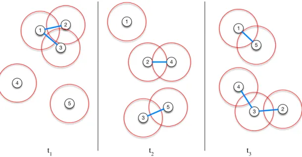
1 2 3 4 5 1 2 3 4 5 1 2 3 4 5 t1 t2 t3
Figure 1: Opportunistic network and three different times. In blue we can see the effective oppor-tunity connections between nodes.
are broken down among the protocols that have some kind of infrastructure support, or based on the nature of its dissemination methods: replication versus forwarding.
The most basic routing algorithm in DTNs is the Direct Contact Algorithm: the source will wait for a direct contact with the destination. When this future encounter occurs, the source will forward the message to the destination. In the k-hop routing scheme, messages are transferred in the DTN through paths consisting of k hops
The epidemic routing [19] is the most popular and simple replication mode in DTNs. Every time two nodes are in contact they will exchange messages. It is easy to see that the global performance of this method is optimal since any other replication method will use a subset of contacts, hence any contact path will also be considered by the epidemic model. Hence, this method is optimal in terms of delivery ratio when buffers and bandwidth are unbounded.
Spray-and-Wait [20] main idea is to reduce the number of message replicas by a simple decision: the source node will only handle a limited number L of them. At each encounter, the node will spray dL/ke copies, keeping for itself L − dL/ke. This process continues recursively until the node has only one copy left. Then it enters into the wait phase, waiting for a direct contact with the destination to forward the message. In [20], they show that the optimal value for k is 2, calling it Binary Spray-and-Wait. The main problem of this algorithm is its hypothesis of an homogeneous network reducing its adaptability to heterogeneous environments.
The PRoPHET routing [21] was one of the first algorithms to perform limited replication of messages. Each node keeps the probabilities of encounter with other nodes. When nodes are in contact they update and share the probabilities of encounters. These probabilities are transitive and age with time. The replication of a message is done if one node has not already a copy of the message and if the node has a higher probability of meeting the destination of the message.
The work of [22] introduces the Resource Allocation Protocol for Intentional DTN (RAPID). RAPID takes into account the utility of replicating a message as a resource allocation problem. A message is replicated only if the utility of replicating the message is higher than the utility of no replication. Three different metrics are proposed: minimization of the average delay, minimization of missed deadlines and minimization of the maximum delay. To calculate the utilities, nodes need to consider extra information that is distributed in the network (such as: past replications of messages, available bandwidth or expected meeting time among nodes).
BUBBLE Rap is presented in [23] in order to cope with social-based DTNs. Indeed, this routing algorithm exploits the inter-human social structures to perform the forwarding. For this, the algorithm performs a community detection in order to select high ranking central nodes (hubs) in the communities. Those nodes will be later used as relays for messages. In terms of the communities, each node belongs to at least one community. It has a global ranking across the whole system, and a local ranking within its local community. In the forwarding phase, a node first bubbles the message up the hierarchical ranking tree using the global ranking. When this process reaches a node in the same community as the destination node, the local ranking is used to bubble up through the local ranking tree until the destination is reached or the message expires. The DiBuBB algorithm [24] is used to detect communities in a distributed way; it has been shown to have a detection accuracy of 85%.
The MaxProp [25] is a routing protocol adapted for vehicular networks. On these networks, the storage capacity is not a problem, but contact times can be short. Hence, MaxProp prioritizes messages based on the delivery likelihood to a destination and the total hop count. This likelihood is based on previous encounters.
The Context-Aware Routing protocol (CAR) [26] uses context information to define the node that will forward the message to the destination. The choice of the best carrier is done using Kalman filter based prediction and utility theory.
The History Based Opportunistic Routing (HiBOp)[27] identifies the appropriate message repli-cating nodes based on past and current context information. A message is forwarded if the en-countered node’s probability of reaching the destination is higher than with the current node. The source can inject several copies of the message in the network to improve the delivery ratio.
2.2
Temporal Networks
Temporal networks have gained interest in the research community over the last few years consid-ering their great number of potential applications: person to person communications, one to many information diffusion, physical proximity, cell biology, distributed computing, infrastructural net-works, neural and brain netnet-works, ecological netnet-works, economic netnet-works, citation netnet-works, etc. Many static representations have been proposed to characterize such temporal networks: reachabil-ity graphs, line graphs, transmission graphs, etc. Also several models producing temporal graphs have been proposed: temporal exponential random graphs, models for social groups, contact net-work models, randomized edges, randomized times, randomized contacts, etc. The problem of rumor-spreading on temporal networks has gained interest, specially to determine how the process is affected by burstiness or temporal and infrastructural inhomogeneities. A complete review on temporal networks, and all the topics discussed above can be found in [28].
A characterization of dynamic mobile networks is presented in [29]. This work presents a frame-work to analyze two real-world datasets in depth, focusing in the study of dynamic communities. The paper presents results for the temporal correlation of the most typical graph properties, such
as: active links, number of connected vertices, average degree, number of connected components and number of triangles.
A time-varying graph model is introduced in [30]. The model is represented by a tuple T V G = (V, E, T, ρ, ψ), where ρ is the presence function, defined as above, and ψ is the latency function which indicates the time it takes to cross a given edge if starting at a given time. From this model a complete description of the properties of TVGs is presented, including: journeys, topological distance, temporal distance, subgraphs, classes of TGV and others.
The small-world phenomenon is defined by networks with a high clustering coefficient and low shortest path length. This is an intrinsic property of many real complex static networks [31]. The work in [32] presents a model capable of capturing the small-world behavior for dynamic networks. They state one sufficient condition to the emergence of a small-world structure in temporal net-works. They also show how this structure significantly improves the communication capacity of opportunistic networks.
Finally, [33] introduces a study on the evolution of graphs over time and their densification laws. This work is more centered on the evolution of big graphs, such as patent networks, evolution of autonomous systems and citation networks.
2.3
Random Walks Meet Temporal Networks
Multiple random walk on static graphs [34] introduces the idea of variability in the starting point in order to avoid some known bias of random walks. The introduction of more walkers with different starting points, and the mixing of the sampled data. The main idea behind this work is to sample some characteristic on static graphs as the average degree.
Random walks on temporal networks were introduced in [35]. This work provides an empirical analysis for different social gathering datasets. This work shows that known characteristics from random walks on static graphs, as the mean first-passage time (MFPT) and the coverage of the ran-dom walk, can be extended to the temporal case. To ensure the convergence of the approximations, the traces are repeated following tree strategies: sequence replication, sequence randomization and statistically extended sequence. They show that the convergence exists in the case of sequence ran-domization. Indeed, the fact of removing the social ties among contacts allows to see the temporal network as a static one.
Our work is inspired on a mix of ideas from the work of [34] and [35]. One important difference is our independence of the underlying temporal network. Indeed, most of the analytical work assumes the evolution of the networks to be an ergodic or Markovian process in order to obtain the distributions. Instead, we do not take into account any underlying nature of the network evolution. We provide a statistical analysis to support our results.
The work in [36] looks at the effects of non-Poisson inter-event statistics on the dynamics of edge. The traditional aggregation of edges to create a static weighted network implicitly assumes that the edges are governed by Poisson processes. This is not typically the case in empirical temporal networks. They apply the concept of a generalized master equation to the study of continuous-time random walks on networks. They discuss the implications for dynamical processes on temporal networks and for the construction of network diagnostics that take into account their nontrivial stochastic nature.
The work of [37] studies the use of random walks on temporal networks and the convergence of the cover time when using just one walker. They show that this convergence is exponential in time.
They also show that the lazy random walk1 converges in polynomial time on the size of the graph.
This reinforces the idea that the use of several walkers in the network can improve the obtained results.
The work of [38] studies the behavior of a continuous time random walk on a stationary and ergodic time varying dynamic graph. They show how to calculate the stationary distribution of the walker. However, this is difficult to characterize on general since it depends on the walker rate. They focus on three cases: (i) Time-scale separation: the walker rate is significantly larger or smaller than the evolution rate of the network or (ii) Coupled dynamics: the walker rate is proportional to the evolution rate of the network. (iii) Structural constraints: the degrees of each node belonging to the same connected component are identical. On these cases they express the analytical solution for the stationary distribution of the walker.
Finally, the work of [39] presents the use of random walks to perform searches in time-varying networks. For this study, the rate of evolution of the network and the rate of the walkers are supposed to be in the same time-scale. They propose a Markovian model of evolution for temporal networks and study the stationary state of the random walk and the MFPT. They show that the dynamics of the time-varying networks significantly alter the standard picture attained for dynamical process in static networks. However, new strategies need to be developed in order to deal with such scenarios.
2.4
Applications on Opportunistic Networks
From an application point of view, work on DTNs and opportunistic networks is mostly focused on the routing problematic. Here, we focus in applications on infrastructure based routing and monitoring over opportunistic networks.
Ad-hoc networks were the first mobile networks to explore the use of infrastructure to help routing messages. Most of the research in mixing mobile nodes and infrastructure (hybrid ad-hoc network) study the capacity increases [40, 41]. However, these studies do not present how to route messages nor how to exploit the dynamics of the network.
The works of [42, 43] propose hybrid routing approaches to increase capacity. In the same context [44] present a heuristic to determine where to randomly place base stations in order to increase connectivity. The work of [45] explores several scenarios introducing base stations, wireless mesh and pure mobile networks.
A relay infrastructure for vehicular mobile networks is presented in [46]. They show how the delivery ratio increases thanks to the relay infrastructure. However their relay nodes are static in crossroads.
In ZebraNet [47], base stations are installed in mobile vehicles that periodically move around the park to gather statistics when they meet the zebras. This works as a mobile infrastructure. In SWIM [48], base stations are installed in buoys (static) and also in seabirds (mobile). In DakNet [49], mobile data carriers are implemented using buses, motorcycles and bicycles. However, in all these examples, the infrastructure is defined by an external agent and it is expensive to deploy.
The work in [50] introduces the idea of “crowd computing”. They show how an opportunistic network of mobile devices offers substantial aggregate bandwidth and processing power.
DTN monitoring in [51] provides an extension to well-known aggregation algorithms for con-nected networks. Specifically, how the notion of pair-wise averaging and population protocols apply to the DTN scenario. This work does not offer a mean to measure the estimation error. Instead, the
estimation is just performed over a given amount of time or a number of desired contacts, assuming that the more contacts, the better the estimation will be. Most of the work to characterize a DTN is based on the global estimation of the intercontact time.
In [52] an analytical model is presented that derives the aggregated distribution law from the pairwise intercontact time distributions. This study also shows that the pairwise connection is not exactly mirrored by the aggregated distribution: if we assume that the pairwise distribution follows an exponential law, then the aggregated distribution will follow a power law.
Finally [53] presents a vicinity study to characterize the behavior of a DTN. In this paper, the concept of k-vicinity and k-intercontact are introduced. Trace analysis shows that k-vicinities intercontact time follows power laws with exponential decay after a given time. Moreover, the k-vicinity of size k={2,3} gives enough awareness of its surrounding to a node. This assumption is supported by the existence of groups in the node movements.
3
Opportunistic Networks Modeling in a Nutshell
In order to set the basic vocabulary that will used in the work we introduce the following definitions: Definition 1 (Node). A node is a mobile entity capable to interchange information bi-directionally within a range r with one or more nodes. The set N denotes all the nodes in the network. Nodes will be noted as natural numbers N = {1, 2, 3, . . . , n}.
For the rest of the work, we will assume that the data exchanged between nodes can be trans-mitted in just one contact. To differentiate this case from the typical DTN bundle [54], we introduce the message definition:
Definition 2 (Message). A message is a packet of data that can be exchanged between two nodes in a connection. All the data for the content is contained in this packet. The content will be named, or tagged in order to retrieve it by its name.
We define Opportunistic Network as follows:
Definition 3 (Opportunistic Network). It as a continuous time stochastic process where nodes exploit systematically their mobility to forward messages between themselves. The mobility in-troduces delay when a node cannot forward its message, keeping it in its own buffer. This allows routing protocols to exploit opportunistic contacts, in absence of stable end to end path, as a means to create a temporal path for delivery.
Figure 1 presents such a network in its most general case: nodes move around in the space and whenever they are in contact (given a transmission range) with another they can profit from that opportunity to forward a message. In order to decrease the temporal complexity, we can transform the continuous time reality into a discrete one. For that we define:
Definition 4 (Time window). The time window is the granularity which we use to sample the continuous time to a discrete one. In the following, we denote this time window as ∆ unit of time, the maximum time as T and the discrete time set as Γ = {t1, t2, . . . , tT}.
Definition 5 (Contact trace). A contact trace is the result of the discretization of the continuous time given a ∆ time window. It is a binary vector, where we denote with a 1 when nodes are in contact and a 0 while they are not. Notice that if the total time T that we observe a process is discretized by ∆, then the contact trace is a vector with T /∆ elements.
We use temporal networks to model in a discrete way the opportunistic networks. Temporal networks are in simple terms networks that change their topology over time. The main difference with other computer networks is that the scale of changes is rather high. We can represent this as a series of time changing graphs where the changes follow a stochastic process usually unknown. Definition 6 (Temporal Network). We define a temporal network as a finite set of graph snapshots G = {G1, G2, . . . , GT}, where Gi= (V (t), E(t)) represents the connection graph at time
t ∈ Γ.
For simplicity, in this work we keep the set of nodes V (t) invariable with time: nodes can be connected or disconnected, but they can not appear or disappear (newborn or dead). This restriction can be eliminated considering the final set V as V = ∪t∈ΓV (t) or with a model for the
birth and death processes. The nodes of the graph are defined as the elements in N (nodes in the network) and the edges E(t) are defined as the set of connected nodes at time t. As in static graphs, we can define the matrices A1, A2, . . . , AT as the corresponding adjacency matrices for each graph
in the temporal network. We can now formally define a temporal connections as:
Definition 7 (Temporal connection). We say there is a temporal connection between i and j at time t if (i, j) ∈ E(t) (equivalently (At)i,j= 1). We denote this as i
t
− → j.
In the following we will consider symmetrical connections. We will just refer to one direction of the connection since if we have i−→ j then we also have jt −→ i.t
We can now define a spatio-temporal path in a temporal network as:
Definition 8 (spatio-temporal path). We say there is a spatio-temporal path Pd
s(t0, t00) between
a source s and a destination d between time t0 and t00if ∃l ≥ 2, v = (s, n01, n02, . . . , n0l−2, d) ∈ Vland
t0≤ t0 1< t02< · · · < t0l−1= t00 such as Psd(t0, t00) = s t0 1 −→ n01 t0 2 −→ n02 t0 3 −→ . . . t 0 l−2 −−−→ n0l−2 t0l−1 −−−→ d (1)
Notice from the definition, the spatio-temporal path is not necessarily unique. Also, the same node can appear more than once on the path in different times. A spatio-temporal has a length in space and time.
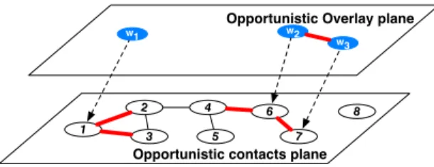
An overlay network is a computer network that is built on top of another network. We can think of nodes in the overlay networks as virtual nodes connected through logical links. These logical links can translate in many links in the underlying network. The most typical examples of overlay networks on Internet today are provided by the distributed hash table of peer-to-peer systems, the XMPP protocol used for Jabber and the numerous implementations of sensor networks in the Internet of Things (IoT). Let us now define an opportunistic overlay network.
Definition 9 (Opportunistic Overlay Network). An opportunistic overlay network is a logical network built on top of the opportunistic network. Nodes and their overlay peers are associated by means of nodes connections in the underlying network. We denote the nodes on the overlay network as W = {w1, w2, . . . , wk}.
An opportunistic overlay network differs from a regular overlay network because it inherits from the non-existence of end-to-end paths as well as of their time-dependence. We now formally define the mapping relation between the two networks (as shown in Figure 2) as:
1 2 7 6 3 w1 w3 w2 8 4 5
Opportunistic Overlay plane
Opportunistic contacts plane
Figure 2: Opportunistic overlay network
Definition 10 (Mapping). A mapping is a relation which associates nodes in the overlay network with nodes in the opportunistic network. Formally we denote m : W → V .
For instance, Figure 2 depicts the mapping relation
m = {(1, w1), (6, w2), (7, w3)}
This mapping relation entails two layers of interactions: the opportunistic contacts plane and the opportunistic overlay plane. In the nodes plane, we see all the existing spontaneous links between nodes, for instance the node 1 is connected with node 2 and the node 3 is connected with node 4. Since node 1 is associated with X by the mapping relation, the latter, in the overlay plane, can capture information of the established connections by 1.
4
Temporal Random Walk over Opportunistic Networks
In this section, we introduce our architecture for the Temporal Random Walk (TRW), we provide an implementation and we explore its connection with message forwarding.
4.1
Architecture of TRW
We can exploit the temporal dimension with the mapping relation. In fact, the mapping can be a function of time in order to follow the evolution of the network dynamics. Hence, in a posterior time, we might see a node in the overlay associated with another node in the opportunistic contacts plane. This leads us to introduce the following distinction:
Definition 11 (Dynamical mapping). A dynamical mapping is a mapping relation that changes with respect to time. We denote such mapping function between an overlay node at a given time as m : W × Γ → V .
Notice that our definition of the dynamical mapping is equivalent to say “who is associated with w at time t”. We can also think in the reverse case: “who is associated with n at time t”2. Given this, we can define our temporal random walk as:
Definition 12 (Temporal random walk). A temporal random walk (TRW) is a dynamical mapping which progression is defined recursively as follows: given an overlay node w ∈ W , a
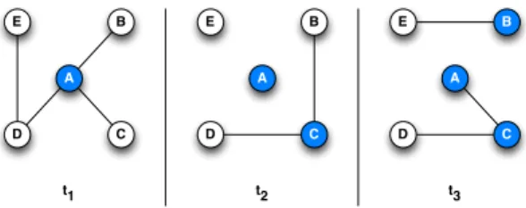
A D B C E A D B C E A D B C E t1 t2 t3
Figure 3: Dynamics of temporal random walks
random starting node i0 = trw(w, 0) and the speed of evolution γ for the TRW. Then, at time
t + γ ∈ Γ the selected node of the TRW is defined as:
trw(w, t + γ) = (
j (i, j) ∈ E(t)
i ∼ (2)
where i = trw(w, t) and j is chosen from the neighbors of i at time t with uniform probability p = 1/δi(t).
For simplicity, we will call a node w in the overlay network a “walker” when it is following a TRW. Also the progression of the TRW will be referred as the step of the TRW.
A temporal random walk differs from a random walk on a static graph as follows: at time t1, a
starting node is randomly selected; after a given time γ one of the nodes’ current neighbors is selected with uniform probability. The probability to pass the token is defined using the temporal degree function δi(t). Hence, if the topology changes, the value of this function may also change
with the time. The process repeats at rate γ from the last selected node. Notice that the rate of the walkers γ may be different from the rate of the network evolution ∆.
In the following we will consider that the pace of the walker is the same as the evolution of the network, hence γ = ∆.
We now introduce the architectural part of our temporal random walk with the following defi-nition.
Definition 13 (Token). A token is a virtual device attached to a walker in the opportunistic overlay network, which is passed from node to node following the steps of the temporal random walk.
For instance, in Figure 3 we see that at time t1 A is selected as the starting node. At this time,
A is connected with {B, C, D}. C is randomly selected with 1/3 probability. Then at time t2 the
connections have changed. We can see that C is connected with {B, D}. In this case B is selected randomly with 1/2 probability. Finally, at time t3E is selected as the only connected node. We see
that the token is passed among nodes in the following contact sequence: {A t1
−→ C, C t2
−→ B, B t3
−→ E} and hence the TRW mapping will be trw = {((w, t1), A), ((w, t2), C), ((w, t3), B)}. We notice two
things: (i) the degree of a node changes with time (δA(t1) = 3, δA(t2) = 0, δA(t3) = 1), hence the
selection probabilities change, and (ii) in the temporal random walk we can profit from temporal paths that are created with the evolution of the communication: the path between A and E only exists thanks to other nodes’ contacts (The temporal path PE
Algorithm 1 Temporal Random Walk algorithm. Notice this function is called at each ∆ time step of the process
1: procedure TRW(nodes) 2: added ← list() 3: for n ∈ nodes do 4: if hasT oken(n) then 5: t ← getT oken(n)
6: if degree(n) > 0 ∧ canRelease(t) then 7: neighbors ← getN eighbors(n) 8: l ← f ilter(neighbors, added) 9: if size(l) > 0 then
10: k ← unif ormSelect(l) 11: put(k, added)
12: passT oken(n, k, t)
Consequently, our definition of the temporal random walk is now equivalent to the following: “which node is holding the token w at time t”. The reverse case will be “which token is the node n holding at time t”.
4.2
Implementation of TRW
The implementation of TRW in a real opportunistic network is a distributed algorithm. At each step of the process, a token holder will (i) exchange synchronization messages with its neighbors; (ii) define the set of neighbors that can receive a token; (iii) pass the token. For simplicity and without loss of generality, we present a centralized version of the algorithm. There are no structural differences between both centralized and decentralized versions. The centralized one keeps a global table at each step to avoid the overhead of probes searching for potential nodes to pass the token to.
The Algorithm 1 presents the implementation details. The TRW procedure is called at each step of the process, and it attempts to pass the token to the node’s neighbors. The TRW builds a list of selected nodes that will hold the token (line 2). For each node in the network, the TRW checks if that node holds a token (line 4). If so, we check if that node is connected to at least one other node and also that it can release its token according to the TRW γ rate (line 6). When more than one token is moving around, we remember that a node can only hold one token at a time. The filter procedure checks which of the connected nodes are holding or will hold the token to remove them from the possible candidates (line 8). Finally, a node is chosen uniformly from one of the filtered neighbors (line 10) and the token is passed (line 12).
The only restriction we impose is that when two token holder nodes meet, they do not exchange their tokens. This contact in the overlay network can be further exploited. In fact, we can merge the tokens information as presented in Algorithm 2. We will call this merge case as TRW-M. It is important to notice that TRW-M is not longer a forwarding method, but also a replication one. Indeed, we can see that in the worst case, we will have as many copies of one message as tokens in the network.
Algorithm 2 Filter algorithm with tokens merging option (TRW-M)
1: procedure filter(neighbors, added) 2: l ← list()
3: for n0∈ neighbors do 4: if ¬hasT oken(n0) then
5: if ¬contains(n0, added) then 6: put(n0, l)
7: else if hasT oken(n0) then 8: mergeT okens(n, n0) 9: return(l)
4.3
Characterization of TRW: Connection with Message Forwarding
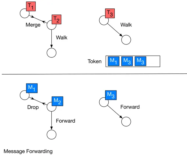
As defined, a temporal random walk is a random walk on a temporal network where one or more walkers carry some messages, perform an action when they meet or gather information. In simple terms, we use the walkers as mobile network nodes and computational devices that move in the network to provide a service. One could think that the token passing between nodes corresponds exactly to the behavior of forwarding a special message in a temporal network. This special message will be passed among nodes indefinitely to distinguish which are the nodes selected by the temporal random walk at a given time. Figure 4 shows the similarities between both processes. When we study the forwarding of a message in an opportunistic network, we can see either two cases: (i) one node holds a message and forward its message to another node that does not have a message (ii) two nodes hold a message and the interchange will produce a drop. We can take advantage of the connection between temporal random walks and message forwarding to characterize the former using the later. Indeed, the forward of the message is equivalent to passing the token. Likewise, the drop of a message can be seen as a merge opportunity for the tokens. In the end, the token is a set of messages that is jumping from one node to another.
An interesting point is to question the real possibility to pass the token at each encounter. This can be characterized in terms of the number of messages in the token. In other words, if we are able to characterize the message drop in the simple message forwarding, we may infer the communication capacity of such temporal random walk.
4.3.1 The (d, c) Model
We consider a temporal network with N identical nodes with a buffer capacity of one message. We consider S < N message sources and M initial copies of the same message. Notice that S = M due to the buffer size restriction. The M messages are delivered to any of D < N − S destinations. Unless stated differently, we consider D = 1. Intermediary nodes act as forwarders of those M messages. Hence, no extra copies are created in the evolution of the process. Our goal is to determine the distribution of dropped messages and the drop ratio over time.
Let 0 ≤ ti,j(1) ≤ ti,j(2) < ... be the successive encounter times among nodes i and j. We
consider that the transmission time of a message is negligible with respect to the time it takes for two nodes to meet one another. It follows that the n-th intercontact time between i and j is icti,j(n) = ti,j(n + 1) − ti,j(n). we assume that the processes {ti,j(k), k ≥ 1, ∀i 6= j ∈ N } are
mutually independent and homogeneous Poisson processes with rate λ > 0. Hence the random variables {icti,j(k), k ≥ 1, ∀i 6= j ∈ N } are mutually independent and exponentially distributed
with mean 1/λ as presented in [55].
Since each node can keep only one message, each time a contact occurs we try to forward it. Hence, when node i and j meet either: (i) only one of the nodes has a message, it is instantaneously transmitted, or (ii) both nodes have a message, then one is chosen at random and it instantaneously transmit its message while the other drops its message.
To calculate the number of dropped messages, we introduce a continuous time Markov chain (X(t), t > 0). The states of the chain are (d, c), where d represents the number of dropped messages and c the number of message copies. Our initial state is when we have M messages to deliver and no drops: (0, M ). The transitions from a generic state (d, c) are:
1. Delivery transition: we transit from (d, c) to (d, c − 1) when a message is delivered. The rate of encountering a destination will be Dλ. Since we have c nodes with a copy of the message, the transition from (d, c) to (d, c − 1) will happen with rate cDλ.
2. Drop transition: we transit from (d, c) to (d + 1, c − 1) when a drop occurs. The transition from (d, c) to (d + 1, c − 1) occurs with rate c(c−1)2 λ given the number of combinations where two nodes with a message meet.
In Figure 5, we detail the possible transitions in the general case. The absorbing states of the chain are in the form (d, 0) with 0 ≤ d ≤ M − 1. Note that when reaching the absorbing states, we must impose some border conditions. Since the last message will be delivered with probability 1, we cannot transit from state (d, 1) to (d + 1, 0).
We can easily calculate the probabilities of going from the state (d, c). Indeed, the embedded Markov chain for X(t) allows to write the probabilities of jumping between states as shown in Equations 3. P ((d, c) → (d, c − 1)) = cDλ cDλ +c(c−1)2 λ= 2D c + 2D − 1 P ((d, c) → (d + 1, c − 1)) = c(c−1) 2 λ cDλ +c(c−1)2 λ= c − 1 c + 2D − 1 (3)
The absorbing states probabilities are defined as:
PM(d) = P (X∞= (d, 0)|X(0) = (0, M )), 0 ≤ d ≤ M − 1 (4)
Since the process is a feed-forward process, these probabilities can be easily calculated with a dynamic programming algorithm. The drop rate distribution is defined as the expected value of reaching the absorbing states over the number of starting messages (Equation 5).
DropRatio(M ) = 1 M M −1 X d=0 d PM(d) (5)
It is important to note that the probabilities are independent of the process arrival rate λ. Therefore, for any {ti,j} defined as before, we expect the same drop ratio results.
4.4
Model Evaluation
In this section, we present the comparison between a simulated opportunistic network and the modeled CTMC results. We generate pairwise ICTs distributed as defined in Section 4.3.1. We then run an event driven simulation to perform the forwarding of the messages in the network and calculate the drop ratio for a given configuration. We compare the simulated and predicted drop ratio for the (d, c) model. The model results have been obtained with MATLAB, while the continuous time simulations are implemented with the R language. We run all the simulations with N = 100 nodes and buffer size B = 1. We repeat each simulation 10 times and provide the average results within a 95% confidence level. The network occupancy is defined as ρ = S/N . Sources are increased to represent the following values of ρ:
ρ ∈ {1, 2, 5, 10, 15, . . . , 80, 95, 98}
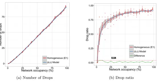
We present the results of simulating with λ = 500. Figures 6a and 6b show how increasing the number of sources (hence the network occupancy) increases the number of messages dropped and the drop ratio as predicted by the (d, c) model. We see in Figure 6a how the model prediction for the drop of messages matches the simulated results. Both grow linearly. Figure 6b presents the drop ratio results. In this figure, we plot the drop ratio for each repetition (red points). We also plot the average interpolation up to a 95% confidence interval envelope (gray area within the error bars). Again, we see how close the simulated and model results are. Indeed, we compute the average case for the 10 repetitions and graph the difference between the average and the model. We see that the maximum difference between both is 0.04. Of course this is only true for the average case. We will see a bigger difference if we include the variance (points dispersion), especially when the number of sources is small: when we have less sources, the probability of dropping a message is lower, but not zero (bigger variance); when we have more sources, the chances of eventually dropping a message are almost 100% (smaller variance).
5
Applications of TRW on Opportunistic Networks
Temporal Random Walks where introduced in Section 4. In this section we study two applications of them in scenarios inspired from the challenges discussed in Section 1.1.
5.1
TRW as a Communication Infrastructure
We present in this section the use of TRW as a lightweight infrastructure to communicate among nodes in opportunistic networks. Given the TRW evolution, each time that a node holds the token in the overlay (walker), the associated node in the opportunistic contact plane can read and write information on it. It is important to note that our algorithm is a generalized version where more than one token can be used in parallel.
5.1.1 Evaluation
We perform a series of simulations with synthetic and real traces using the ONE Simulator [56]. We try the TRW and TRW-M under different scenarios with increasing number of tokens in the network, i.e. |W | = {1, 2, 4, 8, 16, 32}. The message creation process randomly selects a node and adds a new message of 500 kb each 100 seconds. Since we want to study the long term behavior
of the TRW process, we impose that the tokens can store an infinite number of messages and that those messages have infinite time to live.
It is important to remember that TRW-M is a replication method: in the worst case, we will have as many copies of one message as tokens in the network. This is why, we compare our results with the well known Binary Spray-and-Wait [20] routing protocol (BSW), since BSW can define the maximum number L of copies for each message. While the BSW is quite different from our algorithm (restricted message copy at each contact versus token exchange at each contact), we use it as a baseline for comparison in the case of a homogeneous network of nodes sharing the same protocol. Specifically, we compare the average delivery ratio and the average delivery delay using BSW (with increasing number of messages copies {1, 2, 4, 8, 16, 32}). Each BSW node is equipped with a simple broadcast interface of 250 kbps and 10 meters range. A BSW node has a buffer of 5 Mb (10 messages). Note that the BSW with one message is equivalent to direct contact delivery and does not perform as standard BSW.
We assume that the writing and reading time of a message in the token is negligible. Also, merging two tokens is instantaneous (infinite bandwidth). In the following we will consider that the step of the TRW is equal to the update interval of the simulator which is set to ∆ = 1 second. 5.1.2 Synthetic Traces
We use the RandomWayPoint model (RWP) to generate synthetic traces. We have 100 nodes moving with a speed between 0.5 and 1.5 m/s. We simulate three densities of nodes: 103, 104and 105nodes/km2, to show the impact of increasing opportunistic contacts. Each simulation represents
24 hours. We repeat each scenario 10 times to account for variability. We present the mean value in a 95% confidence interval.
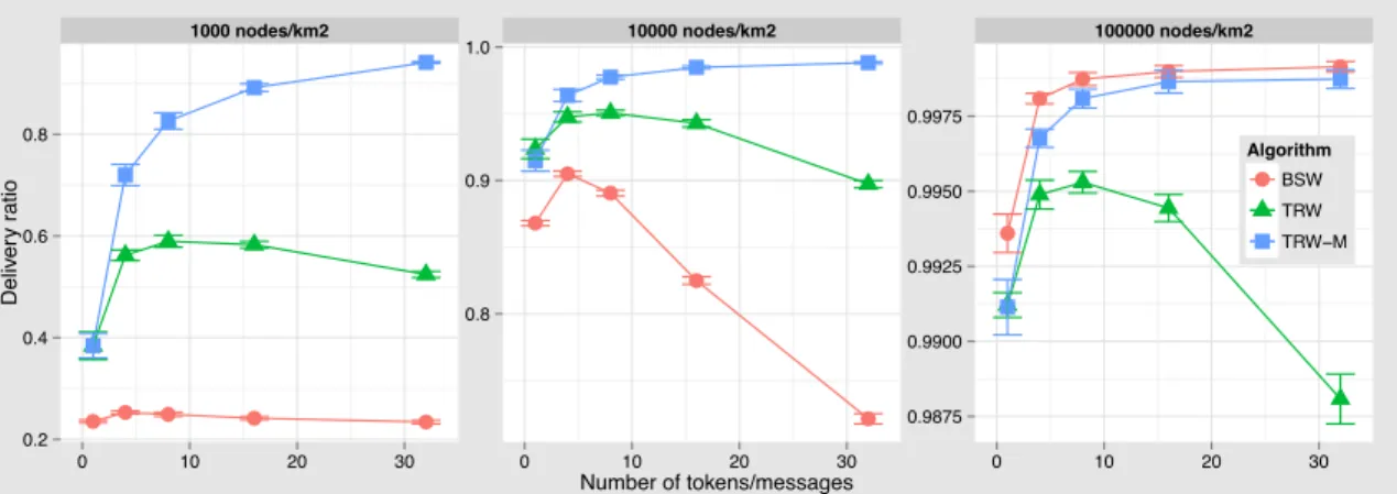
Figure 7 shows that for the highest density scenario, all methods behave similarly. The increasing number of copies in BSW increases the delivery ratio. As expected, adding more tokens increase the delivery ratio as well. Nevertheless, with TRW we see a degradation of the performance in all cases when more than 8 tokens are aggregated. The more tokens that are in the network, the less the token can be passed (due to the restriction of not passing a token to a node that already holds one). This is not the case for TRW-M which profits from tokens interactions to increase the number of messages stored in them. We also see how the BSW is affected when decreasing the density. The lower the density, the fewer contacts, therefore the lower delivery ratio. In the middle density scenario increasing the number of copies has the negative effect of decreasing the delivery ratio from 90% to 70%. This decrease is due to the controlled flooding process of the BSW and the consequent dropping of messages. The dropping occurs when a node exceeds the maximum number of messages on its buffer. In the three scenarios, the TRW-M delivery ratio is maximized with the larger number of tokens. Nevertheless we see that the difference between 4, 8 or 16 tokens is less than 10%.
Figure 8 shows the impact of the number of tokens on the average delay. For the three cases, adding more tokens in TRW adds more delay for the same reason as before: nodes cannot pass the token. In the TRW-M case adding tokens considerably decreases the delay. The delay of BSW is always lower when increasing the number of copies. Even when the delivery ratio is low, the delay is low because only the newest messages are kept in the buffer even though the time to live (TTL) is infinite.
5.1.3 Real Traces
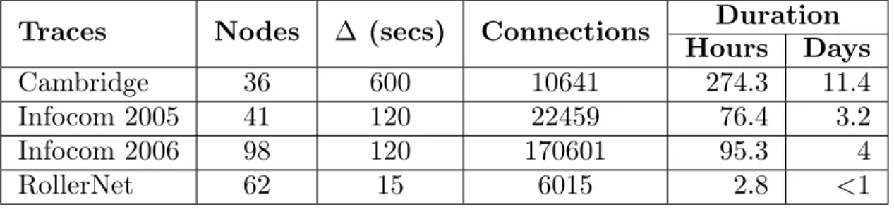
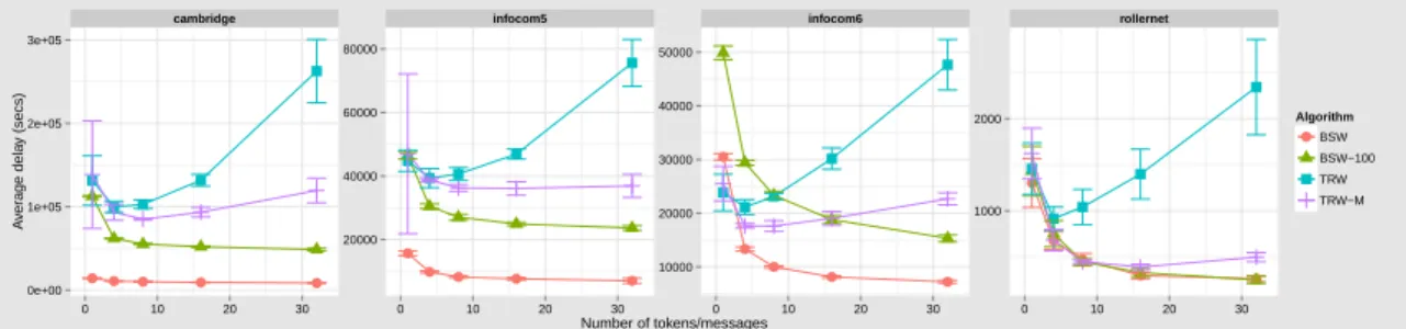
We perform our evaluation using Haggle [57, 58, 59] and RollerNet [60] traces. All are Bluetooth sighting traces by groups of users carrying small devices (iMotes) for a given period. Table 1 summarizes the different traces and their characteristics. Both Infocom experiments were conducted during their respective conferences and workshops trying to capture an opportunistic network in an academic event. The Cambridge experiment investigated the feasibility of a city-wide content distribution architecture composed of short range wireless access points. RollerNet was collected among a thousand participants of a rollerblading tour in Paris. RollerNet studies a class of DTNs that follow a pipelined shape presenting the accordion phenomenon.
As we saw with synthetic traces, the BSW is highly affected by nodes’ buffer size. In this section, we also test the BSW with a 100-message buffer (BSW-100). We repeat each experience 5 times and we present a mean value in a 95% confidence interval.
Traces
Nodes
∆ (secs)
Connections
Duration
Hours
Days
Cambridge
36
600
10641
274.3
11.4
Infocom 2005
41
120
22459
76.4
3.2
Infocom 2006
98
120
170601
95.3
4
RollerNet
62
15
6015
2.8
<1
Table 1: Traces configuration
Figure 10 shows a large variance for the average delivery ratio with just one token for both TRW and TRW-M. This variance decreases as more tokens are added. Also, we see the impact of the buffer size on the BSW. In all Haggle traces we see a boost: Cambridge increases from 15% to 40%, Infocom 2005 from 35% to almost 80% and Infocom 2006 from 40% to 75%. RollerNet is a special case with a higher density of contacts, so here, both versions of BSW performs equally well. We also confirm the degradation in TRW performance above a given number of tokens. In this case we find that between 2 and 4 is the optimal number. It is important to notice that with the Infocom and RollerNet traces with TRW and 4 tokens, we have more than 80% delivery ratio. With Cambridge, the delivery ratio degrades to 63% due the longer duration of the experience. Also as expected, we notice that TRW-M produces the best results in all Haggle traces and in the case of RollerNet, the results are close to those of BSW (less than 10% off). Finally, we notice the stability of TRW: just 4 tokens suffice to get a high delivery ratio.
As expected, the delay of both TRW and TRW-M is larger than that of the BSW (Figure 9). This increase is due to the lack of boundaries of the random walk process with respect to message delivery, i.e. the token moves wherever it can without restrictions. We also confirm that the boost on BSW performance with a bigger buffer also increases the delay. In that case, the nodes are able to store messages for a longer time before dropping them. We see the same increasing delay impact in TRW when adding more tokens, confirming the results from synthetic traces. However, the increase in delay is also associated with an increase in delivery ratio which could be beneficial. When comparing equivalent delivery ratio between TRW-M and BSW, we observe equivalent delays. For instance in RollerNet with 2, 4 or 8 tokens/messages, we confirm that BSW and TRW-M have similar delivery ratio and delay. We see the maximum delay difference with 32 tokens/messages,
Technology Bandwidth Bluetooth 1.0 700 Kbps Bluetooth 2.0 2 Mbps Bluetooth 3.0/4.0 25 Mbps WiFi (device-to-device) 11 Mbps WiFi direct 250 Mbps
USB 2.0 10-280 Mbps (full/hi speed) USB 3.0 3200 Mbps
Thunderbolt 6400 Mbps
Table 2: Typical transfer rates for communication technologies
with an increase of less than 5 minutes. 5.1.4 Cyber-physical considerations
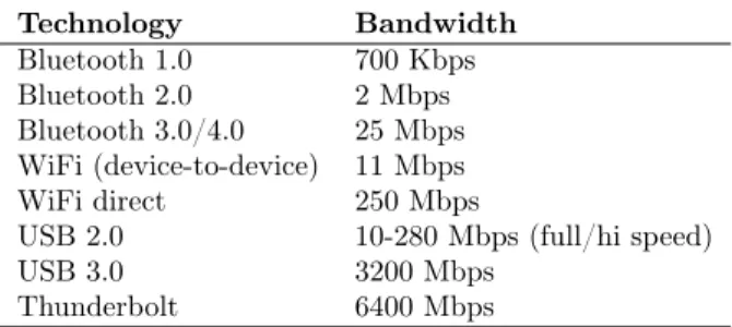
We discuss the cyber-physical aspects associated to a real implementation of TRW. assumptions, limits and benefits of our approach. The main concerns can be grouped in the time needed to read/write in the token (we assume negligible time) and the cost of merging tokens (we assume infinite bandwidth). Both can be explained in terms of technology: the USB key analogy is just a simple example that allows us to devise such a token where the transfer rate is several orders of magnitude greater than current wireless technologies. As we can see in Table 2, our assumption is not far from the reality: Bluetooth 4.0 is 128 times slower than USB 3.0 and 256 times slower than Thunderbolt. Merging messages could be done with the same high speed communication interface among tokens (in the opportunistic overlay plane).
One could also argue that we should count the time of mounting/unmounting the token on the computer, but this is equivalent to someone selecting a file to transfer in a standard manner. Again, we can think of a technology where this process is not cumbersome, e.g. contactless smart cards. Also in terms of storage capacity we know a simple USB key has much more memory than any iMote device of the past.
5.2
Monitoring Opportunistic Networks with TRW: ICT Case
This section introduces the use of TRW to monitor the global Intercontact Time (ICT). We focus on the ICT characterization, since it is a temporal measure that it is highly affected by the quality of the sampled data. We define our notation and explain how to create an approximate characterization of the ICT. We also specify what we understand by ICT approximation.
As defined in section 4.3, the n-th intercontact time between i and j is icti,j(n) = ti,j(n +
1) − ti,j(n). From these random variables, we obtain the pairwise intercontact time distribution
icti,j(t). The global intercontact time ict(t) is defined as ∪i,jicti,j(t). We assume that the pair-wise
distributions for (i, j) and (j, i) are the same. We see that to characterize the global ict(t) we need to know all the pairwise icti,j(t) distributions. Due to the difficulty of gathering all those
pairwise distributions, we propose to select a subset of nodes that can approximate the global ict(t) distribution3.
3We will abuse of the notation for the ict dataset and its associated ict(t) function. We will treat them both as indistinguishable.
Since the ict is defined as a probability distribution, the monitoring problem is reduced to con-struct an estimation of this distribution. We define hicti as the sampling recollected by the moni-toring process. In the following, we propose to investigate methods of providing representative hicti sampling of the whole network. Notice that we can generalize this method to hicti = ∪w∈Whictiw.
5.2.1 Temporal Random Walks to Sample ICT
We propose four sampling strategies for hicti: Static, Last, All, Any. We use a static map for the first strategy and the TRW temporal mapping for the others. Each node in the opportunistic network can store their previous encounters and its frequency. While a node holds the token, it will record the sampled data in the token according to the selected strategy. Then the token will be passed by the temporal random walk and hence the hicti will be collected. Here hicti is constructed as the union of the intercontact values sampled by the token at each connection (i, j). If we have i = (w, t), then:
• Static: we select a random sample S of size k from the set of nodes N . We then define the static map m : wi → i ∀i ∈ S. Note that this relationship is not time-dependent, hence we
can say the monitor nodes are static. It is used as a reference value. All the contacts stored in i will be stored in wi.
• Last: we just consider the last pairwise intercontact between i and all its neighbors. This implies that each node must keep a memory of only the last contact with other node. • All: we consider the complete pairwise intercontact distribution between i and all its
neigh-bors. In this case, the needed memory is extended to all non-recorded contacts in the token. In the worst case this can be all the period of observation.
• Any: we consider the complete history of past intercontact distribution between i and any other node. In this case, we keep the same memory as for the All method.
Now that we are able to define two datasets, the original and the sampled, representing the in-tercontact time distribution of two different groups, we wonder how both distributions are different.
5.2.2 ICT Approximation: How to Compare?
We use the two-sample Kolmogorov-Smirnov (KS) statistical test to compare the sampled hicti with the original ict. The KS test defines a distance D (Equation 6) between these distributions. The Null hypothesis of the two-sample KS Test is if they are drawn from a similar underlying distribution.
D = sup
t>0
|ict(t) − hicti (t)| (6)
We use the p-value to reject the null hypothesis with significance level α = 5%. Rejecting the null hypothesis means that both samples definitely do not come from the same distribution. Failing to reject means that both distributions are the same within an error associated to the significance level.
But, this does not say anything about the distribution they come from. This must be analyzed case by case. Note that this test just says within a given confidence level if the two samples come or not from the same distribution. To go further we need to know specifically which statistical test to perform given the underlaying probability distribution.
5.2.3 Evaluation
In this section, we perform a series of simulations with “The ONE Simulator” [56] to test the intercontact time monitoring strategies previously presented.
Synthetic Traces: For each simulation, we set a group of 100 nodes moving according to the random waypoint movement (RWP) in a square of 100 × 100m2. We gather the approximated
intercontact time distribution according to the four methods. For the simulations, we test N = 100 nodes and ∆ = 5 minutes for T = 500 time windows. Since we want to study the limit of the monitoring methods, for each one, we increase the number of monitors/tokens from 1 to 100. We repeat each simulation 10 times to reduce the randomness effects.
Our initial results indicate that the hicti distribution is similar for both static and dynamic scenarios. We observe that in the RWP simulation each monitor has an indistinguishable view of its surroundings: the monitor sees that all nodes move uniformly into the space. In Figure 11a, the average distance (Equation 6) is graphed as a function of the number of monitors. As expected, we observe that the more monitors we add, the smaller the distance we obtain (hence the better the approximation). This is independent of the method used. Since the homogeneous view in the RWP model, we can say that increasing the number of monitors increases the contacts and hence the quality of the ICT approximation.
Also, we can see that in the one monitor case, it is better to use the dynamic than the static mode. This is due to the fact that we gather more contacts when we move. With the same argument, we can see that the distance between the different strategies in the dynamic mode is correlated with respect to the amount of information we add in the sample: DAny < DAll< DLast.
When calculating the KS test, we always verify the null hypothesis for any number of monitors. This is independently of the selected method (static or dynamic) and sampling strategy selected (Last, All, Any ). In the case of RWP, we know that the ICT [55] follows an exponential law, hence we can fit an exponential model to hicti and obtain the desired result. An overall conclusion can be as such: in the random waypoint scenario, we can monitor a group of nodes using a subset of monitors. The key parameter to take into account is the number of contacts, that can be regulated either by increasing the time sampling or by increasing the number of nodes in the space.
Real Traces: We use the INFOCOM traces [57] to study the 98 distributed nodes in the con-ference. We aggregate the traces into snapshots with ∆ = 5 minutes. We also impose symmetry in the connections. We perform the same analysis than with the synthetic traces. As expected, in Figure 11b, we see that we always decrease the distance between the approximation and the real value of the ICT by adding monitors. However, we see that the Last and All sampling strategies are lower bounded by the Static method. This is equivalent to say that randomly selecting a number of monitors and staying statically attached to them provides a better approximation than dynamically changing nodes when just the pairwise information is considered (as in Last and All strategies). We get a bigger distance due the fact that passing the token at each time can bias the data to smaller values of intercontact time (we will have a higher probability of short intercontact times than the real ict). In the static case we have a partial local view of the network, but consistent with all the periods of observation. This will add longer intercontact times to the sampling, reducing the bias (we will add more information to the tail of the distribution reducing the probability of shorter intercontact times). In other words, adding diversity is not enough to improve the sampling because it adds bias.
However, we can see that the Any sampling strategy always draws the smaller approximation distance. This is due to the fact that this method is a mix between static and dynamic monitoring. Indeed, the holder of the token at the last snapshot will add all its intercontact time information. This information is equivalent to the information that we would have added as a static monitor. However, we have to remember that the cost of this strategy requires that all the nodes in the plane node store theirs contacts. Here the token becomes just a method of data recollection. An obvious improvement is to leverage the monitors connections. When they receive the token they may add their information as well as their past connections information.
Static Any
Statistically representative > 78% > 15% Approximately representative > 17% > 3%
Table 3: Monitors coverage (in percentage of nodes in the network) needed to be sure that hicti is a good estimator for ict (i.e. stop rejecting the null hypothesis)
Both simulation and trace analysis confirm the possibility of selecting a group of nodes and attaching monitors to them in order to capture the global behavior of the ICT. These experiments lead us to conclude that it is not possible to fully define the most representative set of monitors: any non-random selection will introduce some bias to the sampling. Nevertheless, we have not yet explored all the possibilities of our monitoring mechanism. In Table 3, we show the percentage of nodes needed to stop rejecting the null hypothesis (pval > α). To stop rejecting the null hypothesis implies that the hicti is a good estimator for the real ict. We see that in the static case we need to control at least 75% of the network. This implies a huge cost for monitoring. However, in the dynamic case we need only to cover 15% when we use the any sampling strategy. This number hides the fact that all nodes in the nodes plane must be storing past connections in memory. We thus obtain the trade-off sought: either we add more memoryless monitors or we have less monitors to recollect nodes data with higher memory capacity. If we accept a non-statistically accurate view these numbers drop to 17% and 3% respectively. It is important to notice that the fact that the static mapping requires such a big number of monitor nodes is due the unknown dynamics of the opportunistic network. Indeed, since we do not assume any prior knowledge about the nodes, we do not explore nor exploit any specific characteristic that my result in a better selection. In simple words, a random selection will not produce good results. Using this reasoning for the INFOCOM conference, and assuming that the devices delivery was random, we conclude that to get a statistically representative estimation of the ICT , the experience should have covered at least 75% of the people in the conference. We see that the best case is the dynamic mode with the any sampling strategy. This provides the limit of the monitoring: when the monitors plane and the nodes plane become just one, all nodes are constantly monitoring and storing their neighborhood and we use the random walk process just to recollect data.
6
Conclusions
6.1
TRW Architecture for Opportunistic Networks
Random walks on temporal networks were studied in previous work as a sampling method. In this work we used them to provide a computer communication architecture. In Section 4, we defined and discussed the main elements necessary to use temporal random walks over opportunistic networks, defining our own Temporal Random Walk (TRW) architecture. Indeed, we formalized the concept of dynamic overlay for opportunistic networks. We defined a dynamical mapping function that links nodes in the opportunistic network with nodes in the overlay and we defined the token as a virtual device symbolizing who is the walker at a given time. The dynamic mapping is defined at each instant as the nodes in the opportunistic network that are holding a token in the overlay. The progression of the tokens follows a random walk in the temporal network. We then discussed the link between TRW and message forwarding.
6.2
Drop Model for Message Forwarding
DTNs characterization has focused on metrics such as average delay, delivery ratio, etc. assum-ing that the problem of buffer occupancy is of lower importance. In Section 4.3, we studied the drop ratio for the progression of messages from a set of sources to a set of destinations. To our knowledge, we provide the first work specifically focused on the formal analysis of message drop-ping in Opportunistic networks. Each source generates one message that can be absorbed by any destination. Messages in our study are simply forwarded among nodes to avoid the inclusion of extra copies (replication), which will only increase the probability of drops. We worked with nodes with 1-message buffers to represent the worst case scenario to obtain an upper bound for the drop ratio: all nodes in the network have their buffers almost full and we want to know how many new messages can be injected.
Our main contribution is the introduction of a continuous time Markov chain model to character-ize the drop of messages under these hypotheses. We introduced the (d, c) model for homogeneous contact between nodes. We show the link between the encounter rate among nodes with the drop ratio of forwarded messages in the homogeneous case: we showed that the upper bound for the drop ratio is independent of the encounter rate. We performed simulations to calculate the drop ratio for several scenarios to validate the model. We showed that the outputs of the CTMC model fit very well to the simulation outputs. For future work, we plan to better characterize the behavior of the two-class model by varying encounter frequencies. We will further investigate the cases of larger buffers and full heterogeneity.
6.3
TRW as a Lightweight Infrastructure for Opportunistic Networks
As we have discussed in this work, one of the main challenges on opportunistic networks is the lack of persistent end-to-end paths. However, we can exploit temporal paths formed by contacts between nodes. Using the store-carry-and- forward paradigm, nodes can save messages until they find the destination. However, in order to increase the delivery probability, most of the algorithms perform message replication. This naturally introduces overhead as well as complexity for the deployment on opportunistic networks. Many alternatives have been explored in order to reduce the number of copies. For instance, the Binary Spray-and-Wait algorithm introduces a maximum of L copies for each messages. In Section 5.1, we explored the use of temporal random walks over opportunistic networks as a communication infrastructure. We proposed to use contacts as a medium to pass a specific device gathering messages (the token), rather than to route a message. The simple analogy