Détection de changement par fusion d'images de télédétection de résolutions et modalités différentes

(1)

DOCTORAT DE L'UNIVERSITÉ DE TOULOUSE

Délivré par :

Institut National Polytechnique de Toulouse (Toulouse INP) Discipline ou spécialité :

Signal, Image, Acoustique et Optimisation

Présentée et soutenue par :

M. VINICIUS FERRARIS PIGNATARO MAZZEI

le vendredi 26 octobre 2018

Titre :

Unité de recherche : Ecole doctorale :

Détection de changement par fusion d'images de télédétection de

résolutions et modalités différentes

Mathématiques, Informatique, Télécommunications de Toulouse (MITT)

Institut de Recherche en Informatique de Toulouse (I.R.I.T.) Directeur(s) de Thèse :

MME MARIE CHABERT M. NICOLAS DOBIGEON

Rapporteurs :

M. ABDOURRAHMANE ATTO, UNIVERSITE DE SAVOIE CHAMBERY-ANNECY M. PAOLO GAMBA, UNIVERSITA DEGLI STUDI DI PAVIA

Membre(s) du jury :

M. JOCELYN CHANUSSOT, INP GRENOBLE, Président

M. BERTRAND LE SAUX, ONERA - CENTRE DE PALAISEAU, Membre M. JEROME BOBIN, CEA SACLAY, Membre

Mme MARIE CHABERT, INP TOULOUSE, Membre M. NICOLAS DOBIGEON, INP TOULOUSE, Membre

(2)

(3)

(4)

(5)

This thesis would not have been possible without the help, support and guidance of the kind people around me who, in one way or another, contributed and extended their valuable assistance in the preparation and completion of this study. It is a pleasure to convey my gratitude to them all in my humble acknowledgements.

At ﬁrst, I oﬀer my utmost gratitude to my supervisors Prof. Marie Chabert and Prof. Nicolas Dobigeon for their continuous support of my studies and research from the very early stages during the courses at ENSEEIHT until the end of this thesis. They gave me the huge opportunity to conduct my research in their group at the Institut de Recherche en Informatique de Toulouse (IRIT) of the Institut National Polytechnique de Toulouse. I am extremely grateful for their patience, motivation, enthusiasm, and immense knowledge. Their guidance helped me in all the time of research, in writing this thesis and for my personal development. I could not have imagined having better supervisors and mentors for my PhD.

Besides my supervisors, I would like to thank the rest of my thesis committee: Prof. Paolo Gamba, Prof. Abdourrahmane Atto, Prof. Jocelyn Chanussot, Dr Jerome Bobin and Dr Bertrand Le Saux for their encouragement, insightful comments, and hard questions. It has been a great privilege and honour to have them evaluating my work.

This thesis work would not have been successful without the scientiﬁc collaboration of many people. In particular, I would like to thank Dr Qi Wei, Dr Cédric Févotte and Dr Yanna Cavalcanti for all stimulating discussions that helped me with my research.

I would like to acknowledge the ﬁnancial, academic, and technical support of the IRIT and its staﬀ. I thank my fellow labmates at IRIT: Adrien, Louis, Olivier, Alberto, Mouna, Baha, Etienne, Tatsumi, Maxime, Jessica, Dylan, Pierre-Antoine for the stimulating discussions, and for all the fun we have had in the last three years. I could not also forget all the other past and current members of the SC

(6)

Ministry of Education funded me in a 3-year international doctorate program. I hope to have the opportunity of bringing back to Brazil all the knowledge and experience that I have acquired in France since my graduation (also ﬁnanced by the Brazilian government).

Finally, I would like to thank my family for their unending support, encouragement and prayers. Without their support, this work would not have been possible. bove all, I wish to express a very special thanks to you my special friend, dedicated colleague and beloved wife, Yanna Cavalcanti, for all your personal support, for all the time we spent together, for the sleepless nights we were working together before deadlines, for all support you always gave to me, especially in diﬃculties, for all insightful and inspiring discussions, for all your attention even when you were overloaded and for all the love that you have for me. Without you, everything else has no sense.

(7)

La détection de changements dans une scène est l’un des problèmes les plus complexes en télédé-tection. Il s’agit de détecter des modifications survenues dans une zone géographique donnée par comparaison d’images de cette zone acquises à différents instants. La comparaison est facilitée lorsque les images sont issues du même type de capteur c’est-à-dire correspondent à la même modalité (le plus souvent optique multi-bandes) et possèdent des résolutions spatiales et spectrales identiques. Les techniques de détection de changements non supervisées sont, pour la plupart, conçues spécifiquement pour ce scénario. Il est, dans ce cas, possible de comparer directement les images en calculant la différence de pixels homologues, c’est-à-dire correspondant au même emplacement au sol. Cependant, dans certains cas spécifiques tels que les situations d’urgence, les missions ponctuelles, la défense et la sécurité, il peut s’avérer nécessaire d’exploiter des images de modalités et de résolutions différentes. Cette hétérogénéité dans les images traitées introduit des problèmes supplémentaires pour la mise en œuvre de la détection de changements. Ces problèmes ne sont pas traités par la plupart des méthodes de l’état de l’art. Lorsque la modalité est identique mais les résolutions différentes, il est possible de se ramener au scénario favorable en appliquant des prétraitements tels que des opérations de ré-échantillonnage destinées à atteindre les mêmes résolutions spatiales et spectrales. Néanmoins, ces prétraitements peuvent conduire à une perte d’informations pertinentes pour la détection de change-ments. En particulier, ils sont appliqués indépendamment sur les deux images et donc ne tiennent pas compte des relations fortes existant entre les deux images.

L’objectif de cette thèse est de développer des méthodes de détection de changements qui exploitent au mieux l’information contenue dans une paire d’images observées, sans condition sur leur modal-ité et leurs résolutions spatiale et spectrale. Les restrictions classiquement imposées dans l’état de l’art sont levées grâce à une approche utilisant la fusion des deux images observées. La première stratégie proposée s’applique au cas d’images de modalités identiques mais de résolutions diﬀérentes.

(8)

éventuels. La deuxième étape réalise la prédiction de deux images non observées possédant des ré-solutions identiques à celles des images observées par dégradation spatiale et spectrale de l’image fusionnée. Enfin, la troisième étape consiste en une détection de changements classique entre images observées et prédites de mêmes résolutions. Une deuxième stratégie modélise les images observées comme des versions dégradées de deux images non observées caractérisées par des résolutions spec-trales et spatiales identiques et élevées. Elle met en oeuvre une étape de fusion robuste qui exploite un a priori de parcimonie des changements observés. Enfin, le principe de la fusion est étendu à des images de modalités différentes. Dans ce cas où les pixels ne sont pas directement comparables, car correspondant à des grandeurs physiques différentes, la comparaison est réalisée dans un domaine transformé. Les deux images sont représentées par des combinaisons linéaires parcimonieuses des élé-ments de deux dictionnaires couplés, appris à partir des données. La détection de changeélé-ments est réalisée à partir de l’estimation d’un code couplé sous condition de parcimonie spatiale de la différence des codes estimés pour chaque image. L’expérimentation de ces différentes méthodes, conduite sur des changements simulés de manière réaliste ou sur des changements réels, démontre les avantages des méthodes développées et plus généralement de l’apport de la fusion pour la détection de changements.

Mots clés: détection de changements, fusion d’image, multimodalité, image optique multibande, image radar.

(9)

Change detection is one of the most challenging issues when analyzing remotely sensed images. It consists in detecting alterations occurred in a given scene from between images acquired at different times. Archetypal scenarios for change detection generally compare two images acquired through the same kind of sensor that means with the same modality and the same spatial/spectral resolutions. In general, unsupervised change detection techniques are constrained to two multi-band optical images with the same spatial and spectral resolution. This scenario is suitable for a straight comparison of homologous pixels such as pixel-wise differencing. However, in some specific cases such as emer-gency situations, punctual missions, defense and security, the only available images may be of different modalities and of different resolutions. These dissimilarities introduce additional issues in the context of operational change detection that are not addressed by most classical methods. In the case of same modality but different resolutions, state-of-the art methods come down to conventional change detection methods after preprocessing steps applied independently on the two images, e.g. resampling operations intended to reach the same spatial and spectral resolutions. Nevertheless, these prepro-cessing steps may waste relevant information since they do not take into account the strong interplay existing between the two images.

The purpose of this thesis is to study how to more eﬀectively use the available information to work with any pair of observed images, in terms of modality and resolution, developing practical contributions in a change detection context. The main hypothesis for developing change detection methods, overcoming the weakness of classical methods, is through the fusion of observed images. In this work we demonstrated that if one knows how to properly fuse two images, it is also known how to detect changes between them. This strategy is initially addressed through a change detection framework based on a 3-step procedure: fusion, prediction and detection. Then, the change detection task, beneﬁting from a joint forward model of two observed images as degraded versions of two

(10)

images to be spatially sparse. Finally, the fusion problem is extrapolated to multimodal images. As the fusion product may not be a real quantity, the process is carried out by modelling both images as sparse linear combinations of an overcomplete pair of estimated coupled dictionaries. Thus, the change detection task is envisioned through a dual code estimation which enforces spatial sparsity in the diﬀerence between the estimated codes corresponding to each image. Experiments conducted in simulated realistically and real changes illustrate the advantages of the developed method, both qualitatively and quantitatively, proving that the fusion hypothesis is indeed a real and eﬀective way to deal with change detection.

(11)

Introduction 1

I Remote Sensing . . . 1

I.1 Imagery Modalities . . . 2

II Change Detection . . . 6

II.1 A brief historical overview . . . 6

II.2 Change Detection in a remote sensing context . . . 8

II.3 Classiﬁcation according to the supervision . . . 9

II.4 Classiﬁcation according to imagery modality . . . 13

List of publications 23 1 Fusion-based approach 25 1.1 Introduction . . . 25

1.2 Forward model . . . 27

1.2.1 Generic single forward model . . . 27

1.2.2 Multi-band optical forward model . . . 28

1.3 Problem Formulation . . . 30

1.3.1 Applicative scenarios . . . 32

1.4 Proposed 3-step framework . . . 35

1.4.1 Fusion . . . 37

1.4.2 Prediction . . . 38

1.4.3 Decision . . . 39

1.5 An experimental protocol for performance assessment . . . 42

1.5.1 General overview . . . 42

1.5.2 Reference image . . . 45

1.5.3 Generating the HR-HS latent images: unmixing, change mask and change rules 45 1.5.4 Generating the observed images: spectral and spatial degradations . . . 46

1.6 Experimental results . . . 48

1.6.1 Performance criteria . . . 48

1.6.2 Compared methods . . . 50

1.6.3 Results . . . 50

1.6.4 Application to real multidate LANDSAT 8 images . . . 58

1.7 Conclusions . . . 59

2 Robust fusion-based approach 61 2.1 Introduction . . . 61

2.2 Problem formulation . . . 63

2.2.1 Problem statement . . . 63

(12)

2.3.1 Fusion step . . . 68

2.3.2 Correction step . . . 70

2.4 Algorithmic implementations for applicative scenarios . . . 70

2.4.1 Scenario S1 . . . 71 2.4.2 Scenario S2 . . . 74 2.4.3 Scenario S3 . . . 75 2.4.4 Scenario S4 . . . 77 2.4.5 Scenario S5 . . . 80 2.4.6 Scenario S6 . . . 82 2.4.7 Scenario S7 . . . 84 2.4.8 Scenario S8 . . . 86 2.4.9 Scenario S9 . . . 87 2.4.10 Scenario S10 . . . 88

2.5 Results on simulated images . . . 90

2.5.1 Simulation framework . . . 90

2.5.2 Compared methods and ﬁgures-of-merit . . . 91

2.5.3 Results . . . 92

2.6 Results on real images . . . 94

2.6.1 Reference images . . . 94

2.6.2 Design of the spatial and spectral degradations . . . 97

2.6.4 Results . . . 98

2.7 Conclusion . . . 112

3 Coupled dictionary learning-based approach 115 3.1 Introduction . . . 115

3.2 Image models . . . 117

3.2.1 Forward model . . . 117

3.2.2 Latent image sparse model . . . 118

3.2.3 Optimization problem . . . 120

3.3 From change detection to coupled dictionary learning . . . 121

3.3.1 Problem statement . . . 121

3.3.2 Coupled dictionary learning for CD . . . 123

3.4 Minimization algorithm . . . 125

3.4.1 PALM implementation . . . 126

3.4.2 Optimization with respect to W1 . . . 127

3.4.3 Optimization with respect to ∆W . . . . 128

3.4.4 Optimization with respect to Hα . . . 128

3.4.5 Optimization with respect to S . . . . 129

3.4.6 Optimization with respect to Xα . . . 129

3.5 Results on simulated images . . . 130

3.5.1 Simulation framework . . . 130

3.5.3 Results . . . 132

3.6 Results on real images . . . 135

3.7 Conclusion . . . 140

Conclusions and perspectives 143

(13)

A Appendix to chapter 1 151

A.1 Precision . . . 151

A.1.1 Situation 1 . . . 151

A.1.2 Situation 2 . . . 152

A.1.3 Situation 3 . . . 153

A.2 Results of the Fusion Step . . . . 155

A.2.1 Experimental results . . . 156

A.3 Results of the Detection Step . . . . 159

B Appendix to chapter 2 161 B.1 Precision . . . 161

C Appendix to chapter 3 163 C.1 Projections involved in the parameter updates . . . 163

C.2 Data-ﬁtting term . . . 164

C.2.1 Multiband optical images . . . 164

C.2.2 Multi-look intensity synthetic aperture radar images . . . 165

(14)

(15)

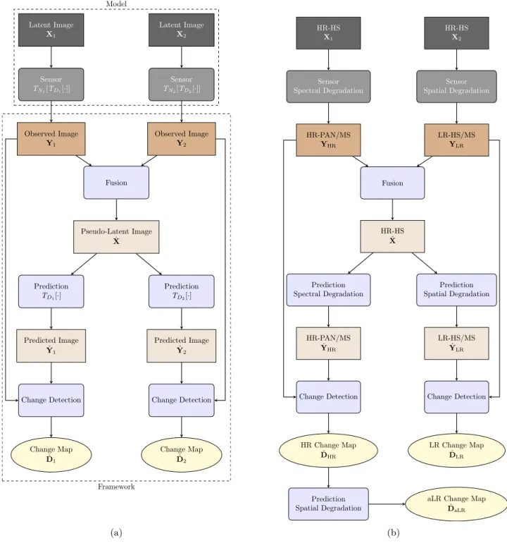
1.1 Change detection framework: (a)general and(b) for S4 . . . 36

1.2 Simulation protocol: two HR-HS latent images X1 (before changes) and X2 (after changes) are generated from the reference image. In temporal conﬁguration 1 (black), the observed HR image YHR is a spectrally degraded version of X1 while the observed LR image YLR is a spatially degraded version of X2. In temporal conﬁguration 2 (grey dashed lines), the degraded images are generated from reciprocal HR-HS images. . . . 43

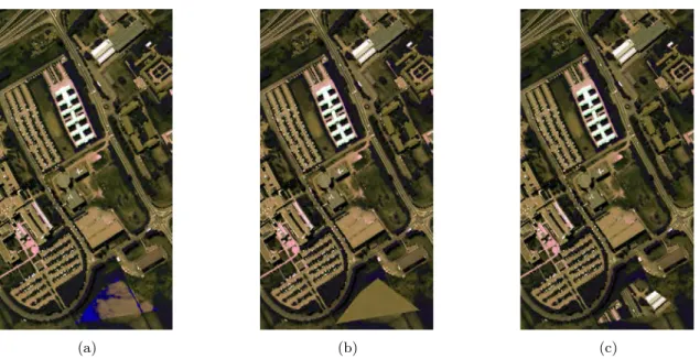
1.3 Example of after-change HR-HS latent images X2 generated by each proposed change rule: (a)zero-abundance,(b) same abundance and(c) block abundance. . . 47

1.4 Degraded versions of the before-change HR-HS latent image X1: (a)spectrally degraded HR-PAN image,(b)spectrally degraded HR-MS image and(c) spatially degraded LR-HS image. . . 48

1.5 Situation 1 (SNR= 30dB): ROC curves computed from(a)CVA,(b)sCVA(7),(c)MAD and (d)IRMAD. . . 53

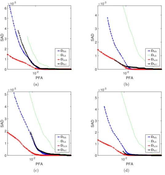
1.6 Situation 1: ∆MSC as a function of the probability of false alarm computed from (a) CVA ,(b)sCVA(7), (c)MAD and (d)IRMAD. . . 54

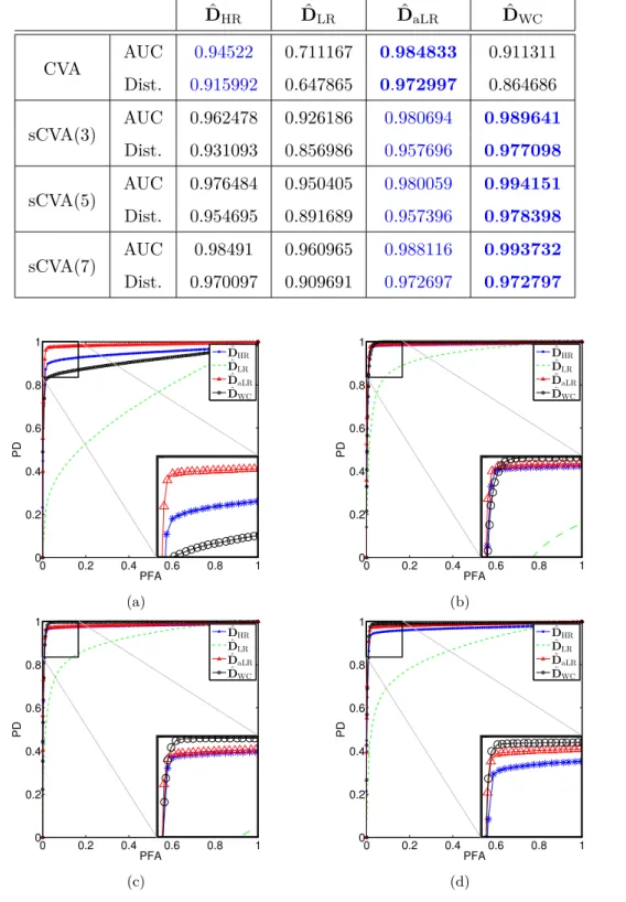
1.7 Situation 2 (SNR= 30dB): ROC curves computed from (a) CVA, (b) sCVA(3), (c) sCVA(5) and(d)sCVA(7). . . 55

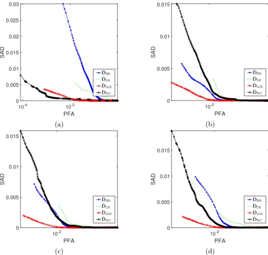
1.8 Situation 2: ∆MSC as a function of the probability of false alarm computed from (a) CVA ,(b)sCVA(3), (c)sCVA(5) and (d)sCVA(7). . . 56

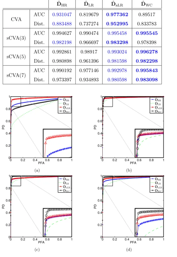
1.9 Situation 3 (SNR= 30dB): ROC curves computed from (a) CVA, (b) sCVA(3), (c) sCVA(5) and(d)sCVA(7). . . 57

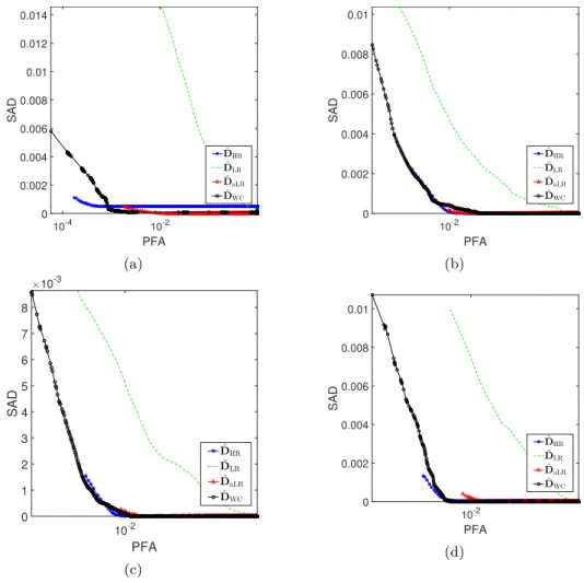
1.10 Situation 3: ∆MSC as a function of the probability of false alarm computed from (a) CVA ,(b)sCVA(3), (c)sCVA(5) and (d)sCVA(7). . . 58

1.11 Real scenario (LR-MS and HR-PAN): (a) LR-MS observed image YLR, (b) HR-PAN observed image YHR, (c) change mask ˆDHR, (d)change mask ˆDaLR,(e) change mask ˆ DWC estimated by the worst-case approach. From (f) to (j): zoomed versions of the regions delineated in red in(a)–(e). . . 59

2.1 Situation 1 (HR-MS and LR-HS): ROC curves. . . 92

2.2 Situation 2 (HR-PAN and LR-HS): ROC curves. . . 93

2.3 Situation 3 (HR-PAN and LR-MS): ROC curves. . . 93

2.4 Spectral and spatial characteristics of real (green) and virtual (red) sensors. . . 95

2.5 Scenario S1: (a)Landsat-8 15m PAN observed image Y1 acquired on 04/15/2015, (b)

Landsat-8 15m PAN observed image Y2acquired on 09/22/2015,(c)change mask ˆDWC

estimated by the WC approach from a pair of 15m PAN degraded images, (d)change mask ˆDF estimated by the fusion approach from a pair of 15m PAN observed and

predicted images and(e)change mask ˆDRFestimated by the proposed approach from a

(16)

2.6 Scenario S1: (a) Landsat-8 30m MS-3 observed image Y1 acquired on 04/15/2015,

(b)Landsat-8 30m MS-3 observed image Y2 acquired on 09/22/2015,(c)change mask

ˆ

DWC estimated by the WC approach from a pair of 30m MS-3 degraded images, (d)

change mask ˆDF estimated by the fusion approach from a pair of 30m MS-3 observed

and predicted images and (e) change mask ˆDRF estimated by the proposed approach

from a 30m MS-3 change image ∆ ˆX. From (f) to (j): zoomed versions of the regions delineated in red in(a)–(e). . . 100

2.7 Scenario S1: (a)AVIRIS 15m HS-224 observed image Y1 acquired on 04/10/2014, (b)

AVIRIS 15m HS-224 observed image Y2acquired on 09/19/2014,(c)change mask ˆDWC

estimated by the WC approach from a pair of 15m HS-29 degraded images,(d)change mask ˆDF estimated by the fusion approach from a pair of 15m HS-29 observed and

30m MS-3 change image ∆ ˆX. From(f)to(j): zoomed versions of the regions delineated in red in(a)–(e). . . 100

2.8 Scenario S2: (a) EO-1 ALI 10m PAN observed image Y1 acquired on 06/08/2011,

(b)Sentinel-2 10m MS-3 observed image Y2 acquired on 04/12/2016,(c)change mask

ˆ

DWC estimated by the WC approach from a pair of 10m PAN degraded images, (d)

AVIRIS 15m HS-29 observed image Y2 acquired on 04/10/2014,(c)change mask ˆDWC

estimated by the WC approach from a pair of 15m PAN degraded images, (d) change mask ˆDF estimated by the fusion approach from a pair of 15m HS-29 observed and

15m HS-29 change image ∆ ˆX. From(f)to(j): zoomed versions of the regions delineated in red in(a)–(e). . . 102

2.10 Scenario S3: (a) Sentinel-2 10m MS-3 observed image Y1 acquired on 10/29/2016,(b)

EO-1 ALI 30m MS-3 observed image Y2 acquired on 08/04/2011, (c) change mask

ˆ

2.11 Scenario S3: (a) Sentinel-2 10m MS-3 observed image Y1 acquired on 04/12/2016,(b)

Landsat-8 30m MS-3 observed image Y2 acquired on 09/22/2015, (c) change mask

ˆ

change mask ˆDF estimated by the fusion approach from a pair of 15m PAN observed

and predicted images method and (e) change mask ˆDRF estimated by the proposed

approach from a 15m MS-3 change image ∆ ˆX. From(f)to(j): zoomed versions of the regions delineated in red in(a)–(e). . . 104

(17)

2.13 Scenario S4: (a)EO-1 ALI 10m PAN observed image Y1 acquired on 06/08/2011, (b)

ˆ

2.15 Scenario S5: (a) EO-1 ALI 30m MS-3 observed image Y1 acquired on 08/04/2011,

(b) AVIRIS 15m HS-29 observed image Y2 acquired on 04/10/2014, (c) change mask

ˆ

change mask ˆDF estimated by the fusion approach from a pair of 15m HS-29 observed

approach from a 15m HS-29 change image ∆ ˆX. From(f)to(j): zoomed versions of the regions delineated in red in(a)–(e). . . 106

(b) AVIRIS 15m HS-29 observed image Y2 acquired on 09/19/2014, (c) change mask

ˆ

change mask ˆDF estimated by the fusion approach from a pair of 15m HS-29 observed

approach from a 15m HS-29 change image ∆ ˆX. From(f)to(j): zoomed versions of the regions delineated in red in(a)–(e). . . 107

EO-1 ALI 10m PAN observed image Y2 acquired on 08/04/2011, (c) change mask

ˆ

approach from 5m PAN change image ∆ ˆX. From (f) to (j): zoomed versions of the regions delineated in red in(a)–(e). . . 108

2.18 Scenario S7: (a) Sentinel-2 10m MS-3 observed image Y1 acquired on 04/12/2016,

(b)Landsat-8 15m PAN observed image Y2 acquired on 09/22/2015, (c) change mask

ˆ

approach from 5m MS-3 change image ∆ ˆX. From (f) to (j): zoomed versions of the regions delineated in red in(a)–(e). . . 109

2.19 Scenario S8: (a)Landsat-8 30m MS-8 observed image Y1 acquired on 04/15/2015,(b)

ˆ

(18)

(b)Sentinel-2 10m MS-4 observed image Y2 acquired on 04/12/2016,(c)change mask

ˆ

2.21 Scenario S10: (a) Sentinel-2 20m MS-6 observed image Y1 acquired on 04/12/2016,

(b)EO-1 ALI 30m MS-9 observed image Y2 acquired on 06/08/2011,(c)change mask

ˆ

approach from a 10m MS-11 change image ∆ ˆX. From (f) to (j): zoomed versions of the regions delineated in red in(a)–(e). . . 112

3.1 ROC curve on simulated data for Scenario 1 corresponding to two optical images . . . 133

3.2 ROC curve on simulated data for Scenario 2 corresponding to two SAR images . . . . 134

3.3 ROC curve on simulated data for Scenario 3 corresponding to a pair of SAR and optical images . . . 135

3.4 Scenario 1 with Landsat-8 observed image pair: (a) Y1 Landsat-8 MS image acquired

in 04/15/2015, (b) Y2 Landsat-8 MS image acquired in 09/22/2015, (c) change map

ˆ

DCF of the Fuzzy method,(d)change map ˆDRF of the Robust-Fusion method and(e)

change map ˆDPof the proposed method. From(f)to(j): zoomed versions of the regions

delineated in red in(a)–(e). . . 137

3.5 Scenario 1 with Sentinel-2 and Landsat-8 observed image pair: (a) Y1 Sentinel-2 MS

image acquired in 04/12/2016, (b) Y2 Landsat-8 MS image acquired in 09/22/2015,

(c)change map ˆDCF of the Fuzzy method,(d) change map ˆDRF of the Robust-Fusion

method and (e) change map ˆDP of the proposed method. From (f) to (j): zoomed

versions of the regions delineated in red in(a)–(e). . . 137

3.6 Scenario 2 with Sentinel-1 observed image pair: (a)Y1 Sentinel-1 SAR image acquired

in 04/12/2016, (b)Y2 Sentinel-1 SAR image acquired in 10/28/2016, (c) change map

ˆ

DCF of the Fuzzy method and(d) change map ˆDP of the proposed method. From (e)

to(h): zoomed versions of the regions delineated in red in(a)–(d). . . 138

3.7 Scenario 3 with Sentinel-2 and Sentinel-1 observed image pair: (a) Y1 Sentinel-2 MS

image acquired in 04/12/2016, (b) Y2 Sentinel-1 SAR image acquired in 10/28/2016,

(c) change map ˆDF of the Fuzzy method and (d) change map ˆDP of the proposed

method. From (e)to(h): zoomed versions of the regions delineated in red in(a)–(d). . 139

3.8 Scenario 3 with Sentinel-1 and Landsat-8 observed image pair: (a)Yt1 Sentinel-1 SAR

image acquired in 04/12/2016,(b)Yt2 Landsat-8 MS image acquired in 09/22/2015,(c)

change map ˆDF of the Fuzzy method and(d)change map ˆDP of the proposed method.

From(e)to(h): zoomed versions of the regions delineated in red in (a)–(d). . . 140

A.1 Situation 1: (a) observed HR-MS image, (b) observed LR-HS image, (c) actual HR CD mask DHR,(d) actual LR CD mask DLR,(e) estimated HR CD map with PFA =

0.0507 and PD = 0.9273 ˆDHR,(f) estimated LR CD map with PFA = 0.2247 and PD

= 0.7592 ˆDLR,(g)estimated aLR CD map with PFA = 0.0486 and PD = 0.9376 ˆDaLR

(19)

A.2 Situation 2: (a) observed HR-PAN image, (b) observed LR-HS image, (c) actual HR CD mask DHR,(d) actual LR CD mask DLR,(e) estimated HR CD map with PFA =

and (h)worst-case CD map with PFA = 0.0876 and PD = 0.9017 ˆDWC. . . 153

A.3 Situation 3: (a) observed HR-PAN image, (b) observed LR-MS image, (c) actual HR CD mask DHR,(d) actual LR CD mask DLR,(e) estimated HR CD map with PFA =

and (h)worst-case CD map with PFA = 0.0876 and PD = 0.9017 ˆDWC. . . 154

A.4 Final ROC curves: (a) Situation 1 and(b)Situation 2. . . 157

A.5 Real situation (LR-HS and HR-HS): (a) LR-HS observed image YLR, (b) HR-PAN

observed image YHR,(c)change mask ˆDFUSEestimated by FUSE approach,(d)change

mask ˆDHySure estimated by HySure approach. From(e)to(g): zoomed versions of the

regions delineated in red in(a)–(d). . . 158

A.6 Change mask: (a)change mask 1, (b)change mask 2 and (c)change mask 3 . . . 159

A.7 Polar CVA for "zero abundance" (top), "same abundance" (middle) and "block abun-dance" (bottom) change rules: change mask 1 (left), change mask 2 (middle), change mask 3 (right). . . 160

B.1 CD precision for Situation 1 (HR-MS and LR-HS): (a) HR-MS observed image YHR,

(b) LR-HS observed image YLR, (c) actual change mask DHR, (d) change mask ˆDRF

estimated by the robust fusion-based approach, (e)change mask ˆDF estimated by the

(20)

(21)

1.1 Overviews of the spectral and spatial degradations w.r.t. experimental scenarios. The symbol − stands for “no degradation”. . . 33

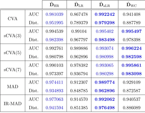
1.2 Situation 1 (SNR= 30dB): detection performance in terms of AUC and normalized distance. . . 52

2.1 Overview of the steps of the AM algorithm w.r.t. applicative scenarios. . . 71

2.2 Situations 1 , 2 & 3: quantitative detection performance (AUC and distance). . . 92

2.3 Pairs of real and/or virtual images, and their spatial and spectral characteristics, used for each applicative scenario. . . 98

3.1 Scenarios 1 , 2 & 3: quantitative detection performance (AUC and distance). . . 133

(22)

(23)

Context

I. Remote Sensing

Remote sensing has many definitions depending on the intended application. Usually, it is considered as the act to acquire information about an object without being in physical contact with it [EV06]. In some more restrictive approaches, remote sensing consists in analyzing the electromagnetic signals radiated or reflected from various objects at ground level (e.g. land, water, surfaces) from a sensor installed in a space satellite or in an aircraft [Che07]. The essential meaning behind all those definitions can be clearly perceived as the gathering of information about the Earth at a distance by analyzing the radiations in one or more bands of the electromagnetic spectrum [CW11].

The remote sensing information acquisition is usually based on the detection or measurement of alterations caused by an object or phenomenon in a surrounding ﬁeld [EV06]. Remote sensing infor-mation combined with other sources of inforinfor-mation, for example, the geographic inforinfor-mation system (GIS) and global positioning system (GPS), produce the concept of geospatial data [CW11]. This concept expand the scope of classic remote sensing applications to more specialized ones, such as: mapping of the evolution of payment of state taxes, mapping uranium enrichment sites, optimizing telecom network capacity, among others.

The remote sensing process can be seen in a twofold scale: macro and micro. The former can be understood as a panorama of the entire process which can be decomposed into four main elements placed in series [CW11]: physical objects, sensor data, extracted information and applications. The physical object category includes the spotted scene elements such as: building, vegetation, water, and many others. Sensor data includes the different ways, often called modalities, used by the sensors to record the electromagnetic radiation emitted or reflected by the landscape. The next block, includes the different ways to highlight important information. The application block refers to the use of the

(24)

remote sensing data in the solution of some practical problem, such as: land-use, mineral exploration, etc.

Although each particular block is composed of complex interrelated processes which also represent important ﬁelds of study. The micro scale vision of the remote sensing process corresponds to a multilevel analysis for each macro block. For instance, the sensor data category can be decomposed in micro scale categories such as: source of energy, propagation through the atmosphere, interaction with the surface physical objects, retransmission of energy through atmosphere, sensor. The information extraction block, can be also subdivided into sensing product, data interpretation and data analysis.

I.1. Imagery Modalities

The most common remotely sensed data is image, which can be explained by its high number of applications. Depending on the scale, macro or micro, imagery can be diﬀerentiated, for instance, by the way the sensor captures the data, the kind of information that is represented and so on. It is common to classify remote sensing images according to physical quantities describing the observed scenes, or classically to the modality.

This classification can be performed according to the used portion of the electromagnetic spectrum. Remote sensing imaging techniques cover the whole electromagnetic spectrum from low-frequencies to gamma-ray [EV06]. The interpretation of the collected data rely on a prior knowledge of the interaction between the electromagnetic signal, the Earth surface and the atmosphere. In this sense, there are three basic models for remote sensing imagery [RJ06; CW11]: i) sensing the reflection of solar radiation from Earth’s surface; ii) sensing the radiation emitted from the Earth’s surface; and iii) sensing the reflection, refraction or scatter of an instrumentally generated signal on the Earth’s surface. The first and the second sensing models are referred to as passive since they are subject to an external energy source, the Sun and the Earth respectively. This is the case when working with ultraviolet, visible and near infra-red bands for the first model, and with, thermal infra-red, microwave emission and gamma-ray for the second one. The third model, on the other hand, is referred to as active due to the self energy emission and recording. The most common active emissions are radar or laser illuminations.

The two most common modalities of remote sensing imagery are passive optical and active radar. According to the Union of Concerned Scientists (UCS) satellite database [Con17], they correspond to more than 60% of the totality of Earth observation satellites with optical satellites corresponding to

(25)

85% of that number. Naturally, both are the most deeply explored for many remote sensing techniques. Nevertheless, the remaining ones must not be neglected. Some kind of modalities, such as LiDAR (Light Detection And Ranging), also present resourceful information for remote sensing applications. Following these statistics, this section focus on the two most used modalities, optical and radar.

Optical Images

Optical images have been the most studied remote sensing data in all applications. Exploring proper-ties of short-wavelengths (400 to 2500nm), that means of solar radiation/reflection on Earth’s surface, optical images are well suited to map land-covers at large scales [Dal+15]. It is worth nothing that, even if optical sensors measure the radiance of the scene, or the brightness in a given direction toward the sensor, the optical data is usually presented through the reflectance, the ratio between reflected and total power energy. The reflectance is a property of the material which is less subjected to vari-ations due to illumination conditions and atmospheric effects. At different wavelengths, materials respond differently in terms of reflection and absorption, which offers a mean to classify the land cover types. Consequently, one strategy to taxonomically classify optical images is how precisely they can identify land-cover types or how precisely the sensor samples the reflected incoming spectrum. Indeed multi-band optical sensors use a spectral window with a particular width, often called spectral reso-lution, to sample part of the incoming light spectrum [Lan02; CW11]. Panchromatic (PAN) images are characterized by a low spectral resolution, as they sense part of the electromagnetic spectrum with a single and generally wide spectral window. Conversely, multispectral (MS) and hyperspectral (HS) images have smaller spectral windows, allowing part of the spectrum to be sensed with higher precision. Multi-band optical imaging has become a very common modality, boosted by the advent of new high-performance spectral sensors [CCC09]. There is no specific convention regarding the num-bers of bands that characterize MS and HS images. Yet, MS images generally consist of a dozen of spectral bands while HS may have a lot more than a hundred. In complement to spectral resolution taxonomy, one may describe multi-band images in terms of their spatial resolution measured by the ground sampling interval (GSI), e.g. the distance, on the ground, between the center of two adjacent pixels [Dal+15; EV06; CW11]. Informally, it represents the smallest object that can be resolved up to a specific pixel size. Then, the higher the resolution, the smaller the recognizable details on the ground: a high resolution (HR) image has smaller GSI and finer details than a low resolution (LR) one, where only coarse features are observable.

(26)

Each image sensor is designed based on a particular signal-to-noise ratio (SNR). The reflected incoming light must be of sufficient energy to guarantee a sufficient SNR and thus a proper acquisition. To increase the energy level of the arriving signal, either the instantaneous field of view (IFOV) or the spectral window width must be increased. However these solutions are mutually exclusive. In other words, optical sensors suffer from an intrinsic energy trade-off that limits the possibility of acquiring images of both high spatial and high spectral resolutions [Pri97; EV06]. This trade-off prevents any simultaneous decrease of both the GSI and the spectral window width. HS, MS and PAN images are, in this order, characterized by an increasing spatial resolution and a decreasing spectral resolution.

Independently of sensor modality, noise is an inevitable phenomenon introduced at different stages during the image acquisition process. Considered as a random process, it can be characterized using the knowledge of the sensor properties. In optical images, it originates mostly in optics and photodetectors. Specifically for this modality, two types of noise sources impair the image formation process: the photon noise and the readout noise [Aia+06b; Deg+15]. The former models the random arrival of photons and their random absorption by the photodetector. The number of photons arriving at the photodetector can be modelled as a counting process. It is commonly assumed that it follows a Poisson distribution. Note that this quantity depends on the signal, so that brighter parts of the image present less sensitivity to the number of arriving photons than darker ones. Consequently, the Poisson noise effect can be neglected when the illumination is sufficient. The readout noise, on the other hand, does not depend on the signal and is present independently of the illumination conditions. It stands for the variability in the transfer and amplification of the photoelectron signal and it is characterized by an additive zero mean Gaussian distribution. This model is the most common in passive optical images [Bio+13].

Radar Images

Radar is the acronym for RAdio Detection And Ranging. Active sensors, such as radar, play a dual role: broadcast a directed pattern to a portion of the Earth’s surface and receive the backscatters of that portion [CW11]. In case of radar, microwaves are used to characterize the range, altitude, direction, or speed of interested targets. Diﬀerent from passive sensors, such as optical, active sensors have interesting capabilities of observation and detection under long-distance and any orientation [Zhu12]. As they produce their own illumination, acquisitions can be performed both day and night and under any weather conditions. Knowing the characteristics of the emitted broadcast signal, the

(27)

analysis of the received backscatters, in terms of frequency and polarization shifts, allows to extract, with high precision, the properties of the illuminated surface. These advantages give radar a central role in military surveillance and Earth observation.

Radar systems have many diﬀerent designs including the real aperture side-looking airborne radar (SLAR) and the Synthetic Aperture Radar (SAR). The former is the oldest and the simplest. It basically consists in a platform (classically airborne or maybe satellite) carrying an antenna array with the nadir direction beneath. The antenna array is obliquely pointed to the side of the platform at a right angle to the ﬂight direction acquiring a swath. The latter is the most known form of radar imagery. Basically it tries to increase the resolution power of real aperture by simulating a large antenna using signal processing techniques [Amb05] and considering overlapping sampling of swath acquisitions. As azimuth resolution is inversely proportional to the size of the antenna and proportional to their elevation, increasing their length increases the resolution [CW11].

Because radar is an active sensor, it is possible to control all the parameters of the emitted signal. For instance, the choice of the signal wavelength (in C,K,X or L bands) or even of multiple wavelengths ("multispectral radar") directly affects resolution, soil penetration and absorption, sensitivity and many other aspects [CW11]. Also, the orientation of the electromagnetic field, or polarization modes (Horizontal, Vertical and their combinations), influence the identification of physical properties on the ground [Amb05].

Pixels of SAR images may be represented as complex numbers where the modulus and the argument stand for respectively the amplitude and the phase of the backscattered wave [Tab16]. An additional information related to the surface reﬂectivity can be retrieved through the amplitude squared, referred to as intensity. For optical images, a pixel corresponds to a ground zone, which is often called resolution cell. Its dimensions and radiometry depend on many parameters of the satellite, the radar and the surface.

As for optical images, the radar image formation process is inevitably corrupted by noise. The coherence of signals used to illuminate the scene leads to constructive and destructive interferences in the image [Pre+15b]. Within the resolution cell, some of these interferences cannot be individually resolved causing signiﬁcant changes in the measured intensity [Tab16; CW11]. This phenomenon is called speckle and has a grainy salt-and-pepper appearance on the image. This behaviour was modelled in an homogeneous zone, such that the pixel intensity follows an exponential distribution while the pixel amplitude follows a Rayleigh distribution [Tab16]. In order to attenuate the speckle, a

(28)

process called multi-look SAR images is applied. This process averages either neighbouring pixels on the same image or samples of the same pixel in diﬀerent multitemporal acquisitions with the drawback of resolution decreasing or inaccuracy due to the presence of changes between acquisitions. The multi-look process consider independent and identically distributed (i.i.d) samples with their number called number of views. The ﬁnal multi-look SAR pixel can be modelled as a multiplicative process for either intensity and amplitude with noise following Gamma distribution with unitary mean value and Nakagami-Rayleigh distribution, respectively.

II. Change Detection

The last macro block of remote sensing refers to the use of the remote sensing information. This section is dedicated to expose one of the most important fields of remote sensing, which is change detection (CD). Initially, a general definition of CD is introduced and a brief historical overview about the early developments is provided. Then, turning CD to a remote sensing application, it is classified according to the information paradigm and also according to the target modality. At the end, the motivations for developing this area and the objectives of this work are given.

II.1. A brief historical overview

The verb to change had as ﬁrst etymological meaning to "make diﬀerent" or, lately, "to alter" and dates to the 12th century. Its derived noun, "change", consequently would represent the act or fact of changing. But the idea of CD is far more ancient. Biologically, it is present in one of the most important functions of the human visual system, the perception of motion [Ull79]. Motion detection is directly related to changes in the visual environment that reach an individual’s eye retina [AS95]. The act of observing a scene over a time interval can only be interpreted as a moving scene if changes occur. Consecutively, the baseline for detecting changes, and consequently motion, is intimately connected to the multitemporality of the scene, which means, the time between acquisitions [AKM93]. Thus, the importance of the analysis of multitemporal images [Hua+81].

An important aspect, when dealing with visual changes, is that not all perceived changes can be cast as a relevant change in the observed scene. Changes in the objects of interest result in changes in reflectance values or local textures that should be distinguished from changes caused by other factors such as differences in atmospheric conditions, illumination, viewing angles, soil moisture and difference

(29)

of noise of multitemporal acquisitions [Ull79; Hua+81; Lu+04]. However, the available information about the scene and about the acquisition conditions is sometimes not suﬃcient to perform this distinction. CD is, thus, an important challenge.

In the beginning, the efforts for detecting changes were made through manual comparison of su-perposed images [Lil72]. Going along with the technological progress, the relevance of automatic CD became strong. The very first evidences about automatic CD in the literature dates from the early 60s, [Ros61;She64], with the first discussion about the need for automatic comparison between digital images. Particularly, in [Ros61] the basic problem was split into three main tasks: image registra-tion, CD and localizaregistra-tion, and change discrimination. Also, it emphasized the need for geometric and radiometric corrections in preprocessing phases. [She64] evoked CD in a remote sensing scenario involving two sets of aerial photographs. This paper also pointed out the need to discard uninterest-ing changes. [Kaw71] envisioned the possibility of CD over multimodal collections of data sets, for instance: photographic, infrared and radar, applied to weather prediction and land surveillance. More particularly, this paper addressed the problem of automatic CD between two aerial photographic data in a city planning context. In [Lil72] was proposed a technique for CD between single-look radar images based on normalized cross-correlation as a similarity measure. The evaluation of similarity measures as differencing operators and correlations in LANDSAT 1 optical multispectral images was studied in [BM76]. The work in [PR76], one of the pioneers in CD, was based on features extracted from segmentation onto homogeneous regions. Synthesizing previous works in a concept of multi-temporal image analysis, [Hua+81] discussed numerous applications closely related to CD such as: medical surveillance, industrial automation and behavioural studies.

So far, CD techniques were essentially based on the so-called pixel-based approach, that compares homologous pixels of the two observed images [BB15]. In [Car89], motivated by the ideas and discus-sions in [Kaw71], was represented a feature-based paradigm for CD. In this new paradigm, instead of comparing homologous pixels, the comparison is made on features extracted from both images according to some speciﬁc methodology (involving segmentation, pyramids, etc ). The hypothesis behind this class of techniques states that, in cases where there is no change, homologous features must remain unaltered. For instance, in [Car89] fractal/multiscale image models were employed to detect man-made changes in SPOT satellite images.

The largely diﬀused work, [Sin89], recalls all previous state-of-the-art CD method applied to re-motely sensed data until that time. It represents one of the ﬁrst survey on the topic which categorically

(30)

classiﬁed CD methods according to the main operation used to compare multitemporal data. After that, motivated by the development and the better understanding of capabilities and applications of remote sensing, CD has lived an exponential growth, starting with the seminal works [BS97;NCS98; JK98;RL98;BP99a;BP99b] which became the basis for development of new strategies for CD in the 21st century.

II.2. Change Detection in a remote sensing context

Ecosystems exhibit permanent variations in diﬀerent temporal and spatial scales caused by natural, anthropogenic phenomena, or even the two [Cop+04]. Monitoring spatial variations over a period of time and thus detecting changes is an important source of knowledge that helps understanding the transformations taking place on the Earth’s surface [Lu+04].

Recalling the concept of remote sensing, it is quite easy to understand why CD is considered as one of its most important ﬁelds of study. Multitemporality, repeatability, coverage and quality of images [Sin89] are special attributes that make remotely sensed data suitable for CD. Various examples of its use can be listed, for instance: land-use and land-cover analysis including forest, vegetation, wetland and landscape; urban area monitoring; environmental and wide-area surveillance; defense and security [Car97;Lu+04].

There is not a formal definition of CD in remote sensing context. According to [Sin89], CD can be considered as the process of identifying differences in the state of an object or phenomenon by observing it at different times. It involves the ability of quantifying temporal effects using multitemporal datasets. From an information theory perspective, [BB15], the information in multitemporal data is associated with the dynamic of the measured variables, which is closely related with the changes occurred between successive acquisitions. According to [Lu+04], CD compares the spatial representation of two points in time while controlling the variations that are not of interest. In [Cop+04], CD is related to the capability of quantifying temporal phenomena from multi-date imagery, that are most commonly acquired by satellite-based multi-spectral sensors. More generally, as in [Rad+05], CD is defined as the ability of detecting regions of changes in images of the same scene acquired at different times. From [BB13], CD in remote sensing context can be viewed as the process leading to the identification of changes occurred on the Earth’s surface by jointly processing two (or more) images acquired on the same geographical area at different times.

(31)

to the target application. Nevertheless, given the previous deﬁnitions, it is possible to capture its essence. Recalling the introductory papers, [Ros61] and [She64], and the important surveys, [Hua+81; Sin89;Lu+04], the CD deﬁnition which is considered in the rest of this work is:

Change Detection consists in analyzing two or more multitemporal (i.e. multi-date) remote sens-ing images acquired over the same geographical spot (i.e. same spatial location), in order to spatially locate the physical alterations that occurred in the observed scene.

Note that, according to the previous definition, CD does not involve change type identification [Ros61]. Change type identification is an important part of change analysis, which can use as input the output of CD methods. The two can be understood as complementary. In this sense, it is very important to correctly define the scope of each one in order to propose CD methods. Thus, a CD method, in this work, will correspond to any method that has as input, at least, two remotely sensed observation images and as output a pixel map indicating the spatial location of changes. Besides, all input images must beforehand be preprocessed in order to represent exactly the same region independently on the modality and on the resolution [BB15]. CD techniques should not compare two scenes that are not geographically aligned [Lu+04].

Remote sensing CD methods can be taxonomically divided into different categories: defined by the modality and the supervision. The next sections define these classifications.

II.3. Classification according to the supervision

Nowadays the terms supervised and unsupervised are well understood especially in the context of machine learning and artificial intelligence. In particular, depending on the availability of ground information, CD methods can be classified as either supervised or unsupervised [Sin89; BP02;BB07; BB13]. According to [BP02], supervised CD methods require a certain amount of ground information used in the construction of training sets. Unsupervised CD methods, on the other hand, do not require any prior ground information but work only with the raw images. In [BB15], CD was presented from a data fusion perspective by classifying CD methods depending if the fusion is at decision or feature level. Methods belonging to the former are based on multitemporal image classification, which frequently are tagged as supervised methods. In the latter, methods are generally based on multitemporal image comparison, which are generally classified as unsupervised.

(32)

Supervised Change Detection

This group gathers methods requiring ground reference information. This information is obtained, generally, from in situ sampling, from photointerpretations or from prior knowledge about the scene [BB13]. Most of the methods belonging to this group use supervised or semi-supervised classification [BB15] such as: artificial neural networks (ANN) [Woo+01], support vector machines (SVM) [NC06; Che+11] and Bayesian classifier [BP01]. Besides, it is possible to note that supervised CD is subdivided into three main branches [BB15]: post-classification comparison (PCC) [Sin89; CDP07], supervised direct multidate classification [Sin89; JL92; Pre+15a; LYZ17] and compound classification [STJ96; BP01;BS97;BPS99].

PCC-like methods perform CD by comparing classification maps obtained from the independent classification of each observed image [Sin89]. They require ground information about each observed image in order to properly produce coherent classification. When classification is performed inde-pendently on the two images, problems such as geographical misalignments, atmospheric and sensor differences between scenes can be reduced. Nevertheless, the detection accuracy is extremely depen-dent on the performance of each individual classification. Indeed, it is comparable to the product of the accuracies of each individual classification [Sin89]. The better the classification the better the detection performance.

Supervised direct multidate classification, on the other hand, identify changes from a combined dataset of all observed images [Sin89]. The dataset combination may have different forms, but in general it is a single feature vector containing information about the two images. The premise is that change classes should produce significantly different statistics compared to the no-change class [MMS07;MMS08;Pre+15a;Pre+15b;LYZ17;Xu+15]. These statistics can be derived in a supervised [Pre+15a] and unsupervised way [LYZ17]. Thus, multitemporal data that was treated separately in PCC-like methods can be jointly processed which requires that the detailed benefits of individual processing of PCC methods be carefully analyzed. Nevertheless, the accuracy of the method is not strongly dependent to the classification performance. Besides, some additional constraints about the training set must be evaluated. Training set must be composed of training pixels related to the same points on the ground at the two times. Also, the proportion of pixels for each change class must be similar in order to avoid misclassification [BB15]. This requirements on the training set may restraint the use of such methods in real applications.

(33)

The third class of supervised CD methods are the compound classification-like techniques. The gen-eral idea is to maximize the posterior joint probability of classes for each pixel on the image, therefore, classify pixels as belonging to change or no-change classes. This kind of techniques uses conditional probabilities obtained under different assumptions and from different estimations. Additionally, as in a Bayesian estimation framework, prior information about the classes can be used allowing better separation between classes. Some of the most employed prior information are related to spatial as-sumptions, for instance, Markov random fields (MRF) [BP99b]. Compared to the previous methods, it exploits temporal correlation between datasets by handling the problem jointly. It allows also some flexibilities in terms of dataset construction. For instance, in some techniques, training pixels are not required to belong to the same area on the ground [BPS99;BB15].

Supervised methods have important advantages. They are more appropriate to handle multimodal observed images than unsupervised methods [Pre15]. Moreover, supervised methods usually perform better than unsupervised ones [BB15]. Indeed the required ground information help to better fit the model used to describe changes. Nevertheless, collecting reference data has an associate cost in terms of time and effort, specially when the method requires a lot of information about a large number of images [BB13]. This fact may play against such methods in real applications which impose a small latency time. Indeed, the overall complexity of these methods are higher compared to unsupervised ones. Besides, they are extremely dependent on the training set. Classifiers trained on narrow training sets have better detection performance but with the cost of reduction on scalability. Thus, considering that the number of potential temporal acquisitions on a given area can be high, supervised methods are becoming less appealing from the application point of view.

Unsupervised Change Detection

Unsupervised CD does not rely neither on a human intervention nor on the availability of ground truth information [BB13]. Most of CD techniques belong to this group, because the ground information is rarely available and because of the common need for automatic CD in many applications.

[Sin89] points out that almost all unsupervised CD methods use a simple 2-step methodology: (i) data transformation (optional) and (ii) change location techniques. The ﬁrst step does not involve preprocessing steps as geographical alignment, but rather transform the input data into another space in which a change location technique is applied. In [BM03; BB15], the output of the ﬁrst step is referred to as the change index. The idea, therefore, is that a data transformation technique over both

(34)

observed images produces a change index. From a data fusion perspective, the change index can be seen as the result of a fusion process at a feature level. The second step, then, process the change index by classifying it as belonging to the change/no-change class. Note that, this step, diﬀerently from supervised CD, does not require any ground information.

The summary presented in [Sin89] classifies the first step according to the main mathematical tools used to perform change index extraction. In [Lu+04], these tools are grouped into two main classes: algebraic tools and transformations. The algebraic tools are basically defined by a specific mathematical operation on the data. Univariate differencing [Sin89; Rad+05; BB15; Du+12], ra-tioning [Sin89;Li+15], vegetation index differencing [Sin89;Lu+04], image regression [Sin89;DYK07; Cha+10], change vector analysis [JK98;BB07;BMB12;Dal+08], similarity measures [Alb+07a;Ing03; Tou+09; Fal+13] are example of the most commonly adopted algebraic tools. Such algorithms are relatively simple and straightforward, nevertheless they are vulnerable to unbalanced data (differ-ences in SNR, radiometric values, etc ). On the other hand, transformation methods apply a data transformation which may reduce data redundancy by emphasizing different information in the de-rived components [Lu+04]. Principal component analysis [Sin89; Rad+05; BB15; Du12], Chi-square [DAd+04; RL98; Lu+04] and correlation analysis [NCS98; Nie07; Nie11; MGC11], multiscale trans-form [Del11;Bou+15; LAT15], are example of common transformations used for CD that are robust to SNR variations. The negative point of these methods is that, usually, the change information is very difficult to interpret and to label in the transform domain.

The second step described in [Sin89] consists in identifying changes from the available change index. The most common procedure is the decision thresholding operation [Sin89;Rad+05]. The thresholding operator classiﬁes pixels into change and no change classes. Classically it is done through a manual trial-error-procedure [Sin89]. Nevertheless, some strategies can be used in order to better separate classes by considering important aspects of desired change images. For instance, spatial priors [BP99b; BM03], minimization of the false alarm rate [Tou+09;Cha+10;Nie07], optimal thresholding [RL98], classiﬁcation through maximum likelihood test [BP99a;BP01;Con+03;Cha+07], etc.

One important requirement of unsupervised CD is that it may need preprocessing steps in order to avoid misclassiﬁcation due to unbalanced data [BB15]. Most of algebraic methods lack of robustness with respect to unbalanced data. This kind of preprocessing includes radiometric corrections [Nie+10; Rad+05; YL00], geometric corrections [IG04; Rad+05] and denoising [Del11]. In comparison to supervised CD methods, they can be signiﬁcantly fast and very suitable for real-time applications.

(35)

Nevertheless, the overall detection accuracy can be signiﬁcantly lower. Today, one of the goals of unsupervised CD techniques is to reach supervised change detection performance without the need for ground information.

II.4. Classification according to imagery modality

The second classification of CD methods involves the modality of the observed images. As remote sensing gathers many different types of imagery modalities, each one representing the scene from a specific point of view, specialized methods were developed for each one by exploiting its physical information. Since the different modalities have very different statistical properties, a general CD method which is capable to accurately handle all modalities is hard to envision. Consequently, most of CD methods consider one modality as a target scenario. When resolutions are the same, homol-ogous pixels are absolutely comparable. Therefore, spatial information represented by that pixel is consistent with the homologous pixel in the other image, contributing to the precision of detection. Nevertheless, in some important situations like punctual missions, natural disasters and defense and security, when the availability of data and the time are strong constraints, CD methods may have to handle multimodal observations with different resolutions. Therefore, CD techniques that can handle multimodal observations are needed.

Same Modality

In this class, CD is performed according to the modality. Each modality has its own characteristics that can be explored for CD and also, maybe, its disadvantages. Among all remote sensing imagery modalities, this section is dedicated to the two most common ones, optical and radar imagery, following the same previous strategy.

Optical imagery change detection Optical images represent the most common remote sensing imagery modality. Therefore there exist a large number of CD methods speciﬁcally designed for optical images [BB15]. Some aspects contributes to that situation. First, the human visual system is based on the optical visible electromagnetic spectrum. Visual inspection, which was the ﬁrst CD method, allows straightforward validation of these methods. Besides, the simplicity of the assumed noise statistics operated in favour of this modality.

(36)

must results in significant changes on radiance values [Sin89]. Otherwise, noise, sun angle differences and other optical effects may be classified as changes. To spatially locate significant physical alterations of objects is the main role of CD. For optical images, the most common CD techniques employs a pixel-wise differencing operator in order to locate abrupt changes in radiance [Sin89;Rad+05;BB15]. This operator is a univariate differencing for panchromatic images or multivariate for multiband optical images. In the latter, in order to gather all pixel change information, the spectral change vector (SCV) can be constructed by stacking the differencing for all pairs of homologous bands between bi-temporal multiband optical images. The justification for the use of differencing is related to the assumed additive Gaussian nature of optical image noise as in Section I.1, for both single variate and multivariate cases. It’s worth noting that the additive nature of the noise, the symmetry of its distribution and the pixel independence can be assumed when a sufficient number of photons arrive on the photodetector. Applying such operators produces a differencing image in which values close to zero tend to represent no-change regions while the strong ones (in absolute value) may represent changes. This assumption is widely used by many unsupervised methods, for instance change vector analysis (CVA) [JK98; BB07] and multivariate alteration detection (MAD) [NCS98; Nie07], and for supervised ones, where the feature vector correspond to the differencing image, for instance [BS97].

Multiband optical images, i.e. multispectral or hyperspectral images, appear as interesting infor-mation sources for CD. The investigation of the electromagnetic response in different wavelengthes allow the development of very precise techniques. The first techniques trying to use multiple band in-formation are based on the vegetation indexes [Sin89;Lu+04]. These indexes are computed from near infra-red and visible red bands. By expanding the analysis through all bands, most of CD techniques in hyperspectral images are based on unmixing [Bio+12;TDT16;Cav+17;Cru+18]. The purpose of unmixing is to obtain, for each pixel, its pure components and their proportions. CD based on unmix-ing of HS images performs far better than CD based on differencunmix-ing PAN or MS images. [Liu+15b; Liu+15c] describe techniques based on multitemporal unmixing. In [EIP16] sparse-unmixing with additional spectral library information is applied in order to attain sub-pixel CD. Nevertheless, tra-ditional unsupervised CD methods derived for optical images with a fewer number of bands can still provide some interesting results. In [Liu+12; Liu+14] the CVA technique is adapted to sequentially detect multiple changes in hyperspectral images. Additionally to unmixing, some subspace techniques are also proposed in order to reduce the amount of data in hyperspectral images while keeping the important information, for instance: principal component analysis [Liu+15a], orthogonal subspace

(37)

projection [WDZ13] among others. Naturally, some advanced methods try to mathematically model the properties of the observed surface. Nevertheless, due to the large variability of materials and mod-els, these methods are not scalable to many problems and are generally time-consuming [Lu+04]. This is the case, for example, when quantifying damages in urban areas after natural disasters [FD15a].

CD from Very High Resolution (VHR) optical images is also a real challenge. The idea is very similar to the previous case. By increasing spatial resolution, the amount of information increases. This can be very helpful in order to analyse small spatial details. Nevertheless, all undesired effects of optical images are amplified. Some techniques try to attenuate these effects by adding extra steps such as predictions. For instance, [BMB12] proposes a multi-level framework to perform CD from VHR optical images. [Dal+08;Fal+13] used morphological filters to reduce the number of false alarms due to miscalibrations in urban areas. In [Xu+15], multiscale analysis is applied in order to take into account finer details while keeping the rough estimation of changes.

Although the mentioned strong points and the broad range of applications, CD from optical images suffers form some limitations. Optical images come from passive sensors, therefore, they highly depend on the natural illumination conditions. Differences in weather conditions make CD difficult, especially in the case of high resolution images. Therefore, a careful calibration of the observations is required in order to guarantee accurate detection. Note that, in case of unsupervised CD, this calibration is rarely possible. Moreover, when working with multiband optical images, some bands may not provide any relevant information or even may be inaccurately sensed leading to false detection. In such a case, these bands must be identified and discarded.

Radar imagery change detection During the technological development of remote sensing, radar appeared as a key tool for target detection. Radar imagery is based on the detection of changes in phase and/or energy of the returning pulse compared to the reference one (the standard emission pulse). Although radar imagery corresponds to the second most common remote sensing imagery modality, CD from radar images is a very challenging task. In opposition to optical images, which have intrinsic characteristics that contributes in the development of relatively simple methods, the nature of the radar images is a difficult obstacle to overcome, particularly the data-dependency and the multiplicative behaviour of the noise, as addressed in Section I.1. For instance, in a same image, brighter portions of the image present more fluctuations than darker parts. When dealing with multi-date images, the scenario is even worst. In a same homologous region, there are strong differences