Comparing System Reliabilities with Ill-Known Probabilities

HAL Id: hal-01346452

https://hal.archives-ouvertes.fr/hal-01346452

Submitted on 19 Jul 2016

HAL is a multi-disciplinary open access

archive for the deposit and dissemination of

sci-entific research documents, whether they are

pub-lished or not. The documents may come from

teaching and research institutions in France or

abroad, or from public or private research centers.

L’archive ouverte pluridisciplinaire HAL, est

destinée au dépôt et à la diffusion de documents

scientifiques de niveau recherche, publiés ou non,

émanant des établissements d’enseignement et de

recherche français ou étrangers, des laboratoires

publics ou privés.

Comparing System Reliabilities with Ill-Known

Probabilities

Lanting Yu, Sébastien Destercke, Mohamed Sallak, Walter Schon

To cite this version:

Lanting Yu, Sébastien Destercke, Mohamed Sallak, Walter Schon. Comparing System Reliabilities

with Ill-Known Probabilities. 16th International Conference on Information Processing and

Manage-ment of Uncertainty in Knowledge-Based Systems (IPMU 2016), Jun 2016, Eindhoven, Netherlands.

pp.619-629, �10.1007/978-3-319-40581-0_50�. �hal-01346452�

probabilities

Lanting Yu, S´ebastien Destercke, Mohamed Sallak, and Walter Schon

Sorbonnes universit´e, Universit´e de Technologie de Compi`egne, HEUDIASYC, UMR 7253. 57 Avenue de Landshut. 60280 Compiegne, [email protected]

Abstract. In reliability analysis, comparing system reliability is an essential task when designing safe systems. When the failure probabilities of the system com-ponents (assumed to be independent) are precisely known, this task is relatively simple to achieve, as system reliabilities are precise numbers. When failure prob-abilities are ill-known (known to lie in an interval) and we want to have guar-anteed comparisons (i.e., declare a system more reliable than another when it is for any possible probability value), there are different ways to compare system reliabilities. We explore the computational problems posed by such extensions, providing first insights about their pros and cons.

Keywords: System design, Reliability analysis, Imprecise probability, Compar-ison

1

Introduction

Being able to compare system reliabilities is essential when designing systems. Pro-vided the structure function mapping single component reliabilities to the overall sys-tem reliability is known, this step poses no particular problem (at least from a theoretical standpoint) when failure probabilities are precisely known.

However, in practice, it may be difficult to provide precise assessments of such probabilities, for example because little data exist for the components (they may be issued from new technologies), or because they are given by expert opinions. This typ-ically happens in early-stage phase design of new systems. In such a case, the problem of comparing system reliabilities become much more difficult, both conceptually and computationally speaking.

In this paper, we explore what happens when the component probabilities of func-tioning are ill-known, that is are only known to lie in an interval. Several aspects of reliability analysis have been extended to the case of ill-known probabilities, such as importance indices [8], multi-state systems [4], common cause failure problems [9], . . . Yet, to our knowledge the problem of system reliability comparison remain to be formally studied within this setting.

In Section 3, we extend usual system comparisons (recalled in Section 2) to interval-valued probabilities in two different ways, discussing the theoretical and practical pros and cons of each extension. Section 4 provides a more complex examples than the very simple, illustrative ones provided along the paper. The necessary basics of reliability as well as notations are briefly recalled in Section 2.

2

System modelling and comparison: basics

In this paper, we assume that we want to compare the designs of K systems S1, . . . , SKin

terms of reliability, in order to choose (one of) the safest among them. The kth system will be composed of a set of rk_{components, and a given component can belong to one}

of T populations (types) of components, all components of a population being assumed to have the same stochastic behaviour (i.e., same failure rate).

We will denote by pj∈ [0, 1] the possibly ill-known probability that a component of

type j is functioning, and 1 − pjthe probability that it is inoperative or malfunctioning.

We will also denote by xk_{i, j}

ik ∈ {0, 1} both the ith component of kth system, which is of

type j_ik, as well as its state (xk

i, jik = 0 if malfunctioning, 1 if working). pjik is then the

probability of xk_{i, j}

ik = 1. Table 1 summarises these notations.

Variable Domain Meaning

K Z Number of systems

rk Z Number of components in the kth system

T Z Number of component types (of possible stochastic behaviors) pj [0, 1], j ∈ {1, . . . , T } Probability that a component of type j will be working

xk

i, jik {0, 1} ith component of kth system, of type jik, and its state

Table 1. Notation summary

In this paper, we will assume that we know the structure function φk: {0, 1}rk → {0, 1} of the kth system and that it is written in the “simple” following way:

φk(x_{1, j}k 1k, . . . , x k rk, jrkk) =

∑

_∏

with d_Ak real-valued coefficients (some subsets A can receive dA= 0) that can either be

positive or negative. At least in principle, every system and structure function can be put in the form of Eq. (1), that is a multi-linear form [2]. We also make the classical assumption in reliability that each system is coherent, meaning that φkis increasing1 and that we have the boundary conditions2φk(0, . . . , 0) = 0, φk(1, . . . , 1) = 1. Going from the structure function to the reliability Rkof the system is then quite simple, as it simply consists in replacing xi, jik by the corresponding probability pjik, that is

Rk(pj1k, . . . , pj_rkk) =

∑

A⊆{1,...,rk}

dk_A

_∏

i∈A

pjik (2)

To simplify notations, we will simply note Rk(p_j1k, . . . , p_j

rkk) by R

k_{. Note that R}k _{is a}

function of the probabilities pj, that can appear multiple times for one subset A. Note

that being a coherent system means that the functions Rjare increasing in every variable pj.

1_{If one component goes from failing to working, then the system state can only improve.} 2_{The system works (fails) if all components work (fail).}

Example 1. Assume we have two (very) simple series system (K = 2), a first with two components, a second with three, and three different component types (T = 3). The two first components of each system are of the same type (1 and 2, respectively). The systems are illustrated in Figure 1, and we do have

R1= p1· p2 R2= p1· p2· p3 x1_1,1 x1_2,2 System 1 x2_1,1 x2_2,2 System 2 x2_3,3

Fig. 1. Two simple series systems

Comparing two systems (say, the kth and `th) then comes down to compare their reliabilities Rkand R`. System Skis then said to be preferred to system S`, denoted by

Sk S`, if and only if

Rk> R` (3)

or, equivalently when probabilities pjare precisely known, if and only if

Rk− R`_{> 0. (4)}

Example 2. Let us continue Example 1 by using the precisely valued probabilities p1=

0.8, p2= 0.9 and p3= 0.8. We then have

R1= 0.72 and R2= 0.576 meaning that system S2should be discarded. We also have

R1− R2= p1· p2− p1· p2· p3= p1· p2· (1 − p3) = 0.144.

We can also notice that whatever the values of p1, p2, p3, we will always have S1 S2

(since R1− R2_{is a product of positive terms).}

Let us now investigate what becomes of such a comparison when probabilities pj∈

[p

j, pj] are only known to lie in intervals.

3

Comparing systems with interval probabilities

In this section, we investigate the most natural extensions of Equations (3) and (4) to an imprecise setting. We will see that in the imprecise case, they do no longer coin-cide, and the first extension only provides an approximation of the second one, but is computationally more tractable.

Note that in this paper, we are interested in guaranteed comparisons, that is we want to assess that Skis more reliable than S`when this is true for any values of pj within

[p

j, pj] and for j = 1, . . . , T . For convenience, we will denote byP = × T

j=1[pj, pj] the

Cartesian product of those intervals.

3.1 Interval comparison: definition

A first way to extend the comparison is to compute bounds over Rk_{, obtaining the}

inter-val [Rk, Rk] such that

Rk= inf p_jik∈[p jik,pjik] Rk=

_∑

_∏

_∑

_∏

Where the fact that probability values can be replaced by their corresponding bounds follows from the increasing monotonicity of reliability functions. We can then straight-forwardly extend Eq. (3) by saying that system Sk is interval-preferred to system S`, denoted SkICS`, if and only if

Rk> R`, (7)

that is we are absolutely certain that Skis more reliable than S`. In this case, comparing two systems just come down to make four computations instead of two to get the corre-sponding intervals. If the two intervals overlap, then systems Sk<sub>and S</sub>`_{are incomparable}

according to this criterion.

However, comparison (7) is very rough, in the sense that it will often result in in-comparability of systems, even if it is obvious that one system is preferable to another, as example 3 shows.

Example 3. Let us consider the systems of Example 2 with the following bounds p1∈ [0.7, 0.9], p2∈ [0.8, 1] and p3∈ [0.7, 0.9].

We then obtain the intervals

R1∈ [0.56, 0.9] and R2_{∈ [0.392, 0.81]}

meaning that the system are not comparable according to IC.

3.2 Difference comparison:definition

Interval comparison somehow extends Equation (3), but a second way to extend the precise comparison is to extend Equation (4). Before doing so, let us simplify notations

by adopting the convention that Rk−`:= Rk− R`_{. We can then say that system S}k _is

difference-preferred to system S`, denoted SkDCS`, if and only if the value

Rk−`= inf p<sub>jik</sub>∈[p jik,pjik] p<sub>ji`</sub>∈[p ji`,pji`] Rk− R` (8) = inf p<sub>jik</sub>∈[p jik,pjik] p<sub>ji`</sub>∈[p ji`,pji`]

∑

_∏

∑

_∏

is positive, i.e., Rk−`> 0. In practice, this comes down to ask Rk<sub>to be higher than R</sub>`_for

all possible values of pj, hence it also gives a guaranteed comparison. Example 4 and

Corollary 1 show that this way of comparing systems is actually better than the previous, in the sense that it still gives guarantee but is less conservative. Yet, computing Rk−`can be far from straightforward (in contrast with the case of interval comparison), and we try to characterize in the next section when this task will be easy.

Example 4. Let us apply Equation (7) to Example 3. In this case we have from Exam-ple 2 that R1−2= p1· p2· (1 − p3) and so

R1−2= inf

p1∈[0.7,0.9],

p2∈[0.8,1],

p3∈[0.7,0.9]

p1· p2· (1 − p3) = 0.7 · 0.8 · 0.1 = 0.056

which is indeed quite low, but still higher than zero, hence S1

DCS2, allowing us to

reach a decision where we could not before.

And indeed, we always have the following relation between the two notions: Proposition 1. Rk−`≥ Rk<sub>− R</sub>`

Proof. The inequality infx∈Df(x) + g(x) ≥ infx∈Df(x) + infx∈Dg(x) with x a vector of

values and D a convex set is known to be true. If we define x as the vector of probability values p1, . . . , pT, and take f = Rk, g = −R`, D =P, we get

inf x∈PR k_{(x) − R}`<sub>(x) ≥ inf</sub> x∈PR k<sub>(x) + inf</sub> x∈P−R `_{(x) ≥ inf} x∈PR k_{(x) − sup} x∈PR `_(x)

We then get the following corollary, showing that if Sk_IC S`, then Sk<sub>DC</sub>S`, but not the reverse. Actually, a similar problem is known under the name ”dependency problem” in interval arithmetic, for which many solutions have been proposed [3]. Corollary 1. If Rk− R`> 0, then Rk−`> 0

So Rk−`is definitely a more accurate way of comparing systems. Let us now study a bit the problem of actually computing it.

Remark 1. In imprecise probability theory, a similar relation exists between the maxi-mality decision rule and the interval dominance decision rule [10]. However, two main differences, in terms of optimization problems, between imprecise probabilities and our study are thatP is here an hypercube and that optimization has to be done over non-linear functions in general, while imprecise probabilities is concerned with bounds of expectations over a subset of the unit simplex. Note that we could also search to adapt other imprecise probability decision rules: maximin and maximax extend directly by using Equations (5) and (6), while the notion of E-admissibility may require more in-volved investigation, especially as it is not based on a pairwise comparison scheme. 3.3 Computing Rk−`

In general, Rk_{− R}`_{will be a polynomial in variables p}

j that is neither decreasing nor

increasing in those variables. Computing bounds over such polynomials when variables lie in a hyper-cube (which is our case) is known to be NP-hard [6], hence infeasible in practice. Two solutions are then to look for approximations that remain close to Rk−` but are more tractable (using interval bounds provides a crude approximation), or to identify those sub-cases for which the solution will be easier to find. In this paper, we explore the second alternative, and leave the first for future works.

Before studying in detail how Rk−`can be computed, we have to recall the notions of global monotonicity and of local monotonicity of a function [5] f (x1, . . . , xn) in a

variable xi

Definition 1 (Global monotonicity). Function f (x1, . . . , xn) is globally increasing

(de-creasing) in xi if it is always increasing (decreasing) in xi, irrespectively of the other

variable values.

If f is globally increasing in xi, then its lower and upper bounds are known to be

obtained for xi= xiand xi= xiwhen xi∈ [xi, xi], respectively.

Definition 2 (Local monotonicity). Function f (x1, . . . , xn) is locally increasing

(de-creasing) in xi if it is either increasing or decreasing in xi when the other variables

x1, . . . , xi−1, xi+1, . . . , xnvalues are fixed.

If f is locally monotonic in xi, then its bounds are known to be obtained for xi=

x_i or xi= xi, but which value to take between these two ones depends on the other

variable values, in contrast with global monotonicity (where the value to consider is fixed, whatever the other variable values). A function will be said to be non-monotone in xiif it is not locally or globally monotone in it.

Example 5. Consider the following functions of x1, x2with xi∈ [−2, 1], then the

func-tions

f1(x1, x2) = x1− x2, f2(x1, x2) = −(x1· x2), f3(x1, x2) = x21· x22

are respectively globally, locally, and not monotone in each of their variables. x1(x2)

is globally increasing (decreasing) in f1. f2 is decreasing in x1 (x2) when x2(x1) is

positive, and increasing when x2(x1) is negative (hence the monotonicity depends on

the value of the other variables). f3 is neither locally nor globally monotone in both

variables (i.e., f

Given two systems Sk and S`, we now define the following subsets of component types: – The subsets Tk= { j ∈ {1, . . . , T }|∀pji`, i = 1, . . . , r `<sub>, j</sub> i`6= j} T`= { j ∈ {1, . . . , T }|∀pjik, i = 1, . . . , r k_{, j} ik6= j}

that denote the types of components that are encountered only in system Sk(Tk) or

S`(T`).

– The subset

T`∩k,1= { j ∈ {1, . . . , T }|∃pji`, pji0ks.t. ji`= ji0k= j ∧

∃!i s.t. ji`= j ∧

∃!i0s.t. j_i0_k= j}

that includes all component types that are in both systems, but only once in each of them.

– The subset

T`∩k,+= { j ∈ {1, . . . , T }|∃pji`, pji0ks.t. ji`= ji0k= j ∧

(∃i, i0s.t. ji`= ji0<sub>`</sub>= j ∨

∃i, i0s.t. jik= ji0k= j)}

that includes all component types that are in both systems and appear more than once in at least one of the two systems.

The subsets Tk, T`, T`∩k,1, T`∩k,+form a well-defined partition of the component types in

systems Skand S`. We can then show a first property

Proposition 2. Rk− R`_{is a globally monotonic function in variables p}

j, j∈ Tk∪ T`. It

is increasing (decreasing) in variables pj, j ∈ Tk(pj, j ∈ T`)

Proof. Without loss of generality, let us assume that p1, . . . , pi∈ Tkand pi+1, . . . , pj∈

T`. By assumption, we have

Rk− R`_{= R}k_(p

1, . . . , pi, pj+1, . . . , pT) − R`(pi+1, . . . , pT),

therefore the monotonicity with respect to p1, . . . , pi(pi+1, . . . , pj) depends only of their

monotonicity with respect to Rk(R`), which are known to both be increasing in those variables.

This means that if pi∈ Tkor T`, we know for which value of pithe lower bound is

obtained (p

iif pi∈ Tk, else pi ) . Also note that in the particular case where Tk∩`,1=

Lemma 1. if Tk∩`,1= Tk∩`,+= /0, then Rk− R`= Rk−`

Proof. When Tk∩`,1= Tk∩`,+= /0, there are no shared variables between Rk and R`,

meaning that j = T in proof of Prop 2 and that inf p1,...,pi inf pi+1,...,T Rk− R`<sub>= R</sub>k<sub>(p</sub> 1, . . . , pi) − R `_(p i+1, . . . , p_T)

Proposition 3. Rk− R`_{is a locally monotonic function in variables p}

j, j∈ Tk∩`,1.

Proof. (sketch) We know that both Rkand R` are equivalent to replacing the xk_{i, j}

ik in

Equation (1) by their probability types. If a type piof component is present once (and

exactly once) in each system, this means that for every subset A, pj power will be

either zero or one in the products ∏i∈Akpjik and ∏i∈A`pji` of Equation (2).

There-fore, Rk_{− R}` _{will be a sum of products where p}

j has power zero or one, meaning

that if the other variables p1, . . . , pj−1, pj+1, . . . , pT are fixed, the derivative of Rk− R`

with respect to pj will be a constant (whose positivity or negativity will depend of

p1, . . . , pj−1, pj+1, . . . , pT values), hence that Rk− R`is either decreasing or increasing

in pj. x1 1,1 x12,2 System 1 x2 1,2 x22,3 System 2

Fig. 2. Two simple series systems with common component

Example 6. Let us consider the series systems of Figure 2 with three types of compo-nents, where p2∈ T1∩2,1. We have

R1− R2= p1· p2− p3· p2= p2· (p1− p3)

which is indeed locally, but not globally, monotone in p2(it is increasing if p1> p3,

decreasing if p1< p3).

This means that, if we have N = |Tk∩`,1| variables pjfor which we are locally

mono-tone, we know that the lower bound is obtained for one of the 2Nvertices of the corre-sponding hypercube ×i∈T_k∩`,1[p_i, pi]. If N is not too high, then we can think of simply

enumerating the set of possible values.

Finally, we cannot guarantee any kind of monotonicity for the variables pj, j ∈

T`∩k,+. However, if the cardinality of T`∩k,+ is not too high, it is always possible to

Example 7. Let us consider the very simple case depicted in Figure 3, where we have R1= p2₁and R2= p1

hence R1−2= p2₁− p1= p1(p1− 1), which will always be negative. However, if p1∈

[0.4, 0.6], the bound R1−2= −0.25 is obtained for p1= 0.5, which does not correspond

to one of the bounds p

1, p1.

x1_1,1 x1_2,1

System 1

x2_1,1

System 2

Fig. 3. Two simple series systems with redundancy

It means that when confronted with too much components present in both systems and multiple times in at least one of them, computing the bound may quickly become intractable in practice. This becomes even truer if the monotonicity of other variables (those in T`∩k,1) depends on those variables in T`∩k,+.

An easy solution is to ”duplicate” each variable pjin T`∩k,+with variables having

the same interval bound, so that each variable is present at most once in each system. In the case of Figure 3, this means considering a variable p0₁for the second component of System 1. Such a straightforward approach has two potential drawbacks: the increase of the number of component types in T`∩k,1, and the fact that the approximation can be

quite loose. Such a strategy is therefore likely to be useful only when the number of component types.

4

A more complex example

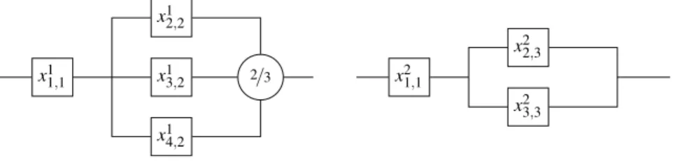
Let us now consider two slightly more complex systems, where we want to chose the most reliable design. The systems are depicted by Figure 4, and consider three types of components, with p1∈ [0.9, 1], p2∈ [0.8, 0.9] and p3∈ [0.85, 0.95], where one hesitates

between choosing a 2 out of 3 architecture with slightly less reliable components, and a parallel architecture with potentially more reliable components. The reliabilities of the systems are

R1= p1· p22· (3 − 2p2)

and

R2= p1· p3· (2 − p3).

Intervals [R1_{, R}1_{] and [R}2_{, R}2_{] intersect, hence interval comparison is not sufficient to}

tell us whether S1is better than S2, or the reverse. We have T1∩2,1= {1}, T1= {2} and

T2= {3}, therefore if we want to compute R1−2, our previous results tell us that

R1−2= p∗₁· p2

2· (3 − 2p2) − p ∗

with p∗₁∈ {p

1, p1}. The result is obtained for p1(the function is decreasing in p1for

p2= p₂and p3= p3), and R1−2= −0.1015, meaning that we cannot conclude that

S1DCS2. Following a similar line of reasoning for R2−1(which is increasing in p1),

we get R2−1= 0.00495 and are able to tell that S2DCS1.

x1_1,1

x1_2,2

x1_3,2

x1_4,2

2_/3

Fig. 4.A: System S1

x2_1,1

x2_2,3

x2_3,3

Fig. 4.B: System S2

Fig. 4. Two system designs to compare.

5

Conclusion

In this paper, we have studied how comparisons of system reliabilities can be extended when probabilities are ill-known, or interval-valued. In particular, we have focused on comparison notions that allows for incomparability when the information is too weak to be certain that one system is more reliable than another.

We have seen that computing the lower bound over the difference of reliabilities is less conservative, but more computationally demanding than just comparing reliability bounds of each systems taken individually. While we have pointed out ways to reduce the complexity of such computations (by focusing on global and local comonotonicity), it remains to investigate how to approximate Rk−`with a lower bound better than Rk− R`, but computationally more tractable than computing Rk−`. A first way to do so is to exploit bounds used when the reliability probabilities are precisely known, but when computing the output probability is computationally prohibitive, see e.g., [7].

An additional interesting problem to explore is to formalize which information we should query to make two incomparable systems comparable. For instance, we may formulate it as an expert elicitation problem [1].

References

1. Abdallah, N.B., Destercke, S.: Optimal expert elicitation to reduce interval uncertainty. In: Proceedings of the Thirty-First Conference on Uncertainty in Artificial Intelligence, UAI 2015, July 12-16, 2015, Amsterdam, The Netherlands. pp. 12–21 (2015)

2. Borgonovo, E.: The reliability importance of components and prime implicants in coherent and non-coherent systems including total-order interactions. European Journal of Opera-tional Research 204(3), 485–495 (2010)

3. De Figueiredo, L.H., Stolfi, J.: Affine arithmetic: concepts and applications. Numerical Al-gorithms 37(1-4), 147–158 (2004)

4. Ding, Y., Lisnianski, A.: Fuzzy universal generating functions for multi-state system relia-bility assessment. Fuzzy Sets and Systems 159(3), 307–324 (2008)

5. Fortin, J., Dubois, D., Fargier, H.: Gradual numbers and their application to fuzzy interval analysis. IEEE Transactions on Fuzzy Systems 16(2), 388–402 (2008)

6. Kreinovich, V., Lakeyev, A., Rohn, J.: Computational complexity of interval algebraic prob-lems: Some are feasible and some are computationally intractable-a survey. Mathematical Research 90, 293–306 (1996)

7. Mteza, P.Y.: Bounds for the reliability of binary coherent systems. Ph.D. thesis (2014) 8. Sallak, M., Schon, W., Aguirre, F.: Extended component importance measures considering

aleatory and epistemic uncertainties. Reliability, IEEE Transactions on 62(1), 49–65 (2013) 9. Troffaes, M.C., Walter, G., Kelly, D.: A robust bayesian approach to modeling epistemic

uncertainty in common-cause failure models. Reliability Engineering & System Safety 125, 13–21 (2014)

10. Troffaes, M.: Decision making under uncertainty using imprecise probabilities. Int. J. of Approximate Reasoning 45, 17–29 (2007)