Any correspondence concerning this service should be sent to the repository administrator:
[email protected]
To link to this article : DOI:
10.1016/j.envsoft.2017.01.007
URL :
http://dx.doi.org/10.1016/j.envsoft.2017.01.007
This is an author-deposited version published in:
http://oatao.univ-toulouse.fr/
Eprints ID: 17481
O
pen
A
rchive
T
oulouse
A
rchive
O
uverte (
OATAO
)
OATAO is an open access repository that collects the work of Toulouse
researchers and makes it freely available over the web where possible.
To cite this version: Douinot, Audrey and Roux, Hélène and Dartus,
Denis Modelling errors calculation adapted to rainfall - runoff model user
expectations and discharge data uncertainties. (2017) Environmental
Modelling errors calculation adapted to rainfall e Runoff model user
expectations and discharge data uncertainties
Audrey Douinot
*, H!
el"
ene Roux, Denis Dartus
Institut de M!ecanique des Fluides de Toulouse (IMFT), Universit!e de Toulouse, CNRS-INPT-UPS, Toulouse France
Keywords: Uncertainty propagation Hydrological modelling Calibration Evaluation Discharge uncertainty Error isolines
a b s t r a c t
A novel objective function for rainfall-runoff model calibration, named Discharge Envelop Catching (DEC), is proposed. DEC meets the objectives of: i) taking into account uncertainty of discharge obser-vations, ii) enabling the end-user to define an acceptable uncertainty, that best fits his needs, for each part of the simulated hydrograph. A calibration methodology based on DEC is demonstrated on MARINE, an existing hydrological model dedicated to flash floods. Calibration results of state-of-the-art objective functions are benchmarked against the proposed objective function. The demonstration highlights the usefulness of the DEC objective function in identifying the strengths and weaknesses of a model in reproducing hydrological processes. These results emphasize the added value of considering uncertainty of discharge observations during calibration and of refining the measure of model error according to the objectives of the hydrological model.
1. Introduction
An objective function converts the outputs of a rainfall-runoff model into a single likelihood measure, according to discharge measurements. This likelihood measure plays a key role, as it controls the model assessment and calibration. As such it provides a comparison basis for models or scenarios. An objective function must provide a meaningful criterion, representative of the errors occurring in the prediction time series. Ideally the objective func-tion must make a distincfunc-tion between the observed errors coming from data uncertainties and the modelling errors coming from model limitations and parameter uncertainties. Defining such a metric is hard, as model outputs obviously depend on the input data and the observed discharge quality.
The uncertainty of the forcing data (rainfall/snowfall, soil moisture, etc.) is in general not measurable (Villarini and Krajewski (2010); Kirstetter et al. (2010)) whereas discharge uncertainties can be accurately quantified (McMillan and Westerberg, 2015;Coxon et al. (2015); Le Coz et al. (2014)). This makes it possible to inte-grate uncertainty of the discharge observationst into an objective function. However the classical functions, such as the Nash-Sutcliffe efficiency (NSE,Nash and Sutcliffe, 1970), or the
Kling-Gupta-Efficiency (KGE, Gupta et al., 2009), are based on the dif-ference between the model outputs and the observed discharge, without considering the discharge uncertainty. This can result in the overfitting of a model prediction to uncertain discharge observations.
Some modifications in different calibration approaches are found in the literature in order to integrate uncertainty of the discharge observations. Croke (2007) modified the NSE by weighting the residual vector according to the accuracy of observed discharge measurement. The metric thus emphasizes the predic-tion of a well known observed discharge at the expense of the observed discharge with high uncertainty. This is especially prob-lematic in the context of flood modelling, where extreme flood discharges are generally marred with high uncertainty. Calibration methods based on Bayesian approach (Kuczera (1983); Engeland and Gottschalk, 2002, Kavetski et al., 2006), formalize an error model, considering among others discharge uncertainty. Formal-izations of different type of errors, such as input uncertainty or model uncertainty are based on strong assumptions that require validation, which is not always possible. In the end, the calibration results depend on the definition of the error model.Liu et al. (2009)
proposed a calibration method using a “limits-of-acceptability” approach. A parametrization is either accepted or rejected. The limit of acceptability is fixed according to discharge uncertainty. The method is convenient to assess the likelihood of a parameter set for a model, but it does not provide information on the
* Corresponding author.
relevance of the model.
The aim of the paper is to provide an objective function: i) taking into account uncertainty of the discharge observations; ii) adapting the calibration to user expectations and model assumptions; iii) providing a meaningful score which can be interpreted to assess the relevance of the model.
Section2 presents the rationale of the paper. It discusses the state of the art of objective functions in the field of hydrologic models, with a focus on the model calibration issue. The proposed objective function, called Discharge Envelop Catching efficiency, is defined in Section3and evaluated against three other objectives functions in Section4. Finally, calibration results are presented and discussed in Section5.
2. Background and motivation
We begin the section introducing the mathematical concepts used throughout the paper.
2.1. Mathematical notation and symbols
We adopt the fomulation ofVrugt and Sadegh (2013)of model calibration and evaluation issues: “Consider a discrete vector of measurements ^Y ¼ { ^y1,
…
, ^yn}, observed at times t ¼ { 1,…
, n } thatsummarizes the response of an environmental system F to forcing variables Û ¼ {û1,…, ûn}. Let Y ¼ {y1,
…
, yn} the correspondingpredictions from a dynamic (non linear) model f, with parameter values
q
,Yð
q
Þ ¼ f!x0;q
;Ub #(1)
where x0 is the initial state of the system at t ¼ 0.” The residual vector defines the difference between actual and model-simulated system behaviours:
Eð
q
Þ ¼ bY $ Yðq
Þ ¼ fe1ðq
Þ; :::;enðq
Þg (2)The error model F that allows for residual vector transformation defines the modelling error vector:
εð
q
Þ ¼ F hb
Y $ Yð
q
Þi¼ fε1ðq
Þ; :::;εnðq
Þg (3)A function G is used to map the modelling error vector into a metric called likelihood measure. The combination of F and G is the objective function.
Calibration aims to find the values of [
q
2Q
2 <d] that provide the best likelihood measure. As the optimal parameter set may not be unique and several candidates may minimized equally the objective function, the calibration process faces model equifinality (Beven and Binley, 1992; Beven, 2006). Choosing a way of selecting or weighting behavioural parameter sets according to likelihood measure corresponds to the last step of a calibration methodology. We now consider the fact that forcing variables Û, initial state x0and observed discharges ^Y are uncertain measurements and denote
s
Û,s
X0,s
Y^ the vectors quantifying those uncertainties. Forcingvariables and initial state uncertainties affect model predictions and modify equation(1):
Y0 ð
q
Þ ¼ f!x0 & & &s
x 0;q
;Ub & & &s
b U # (4)where Y0(
q
) is the model prediction with respect to inputun-certainties. Similarly, the observed discharge uncertainties modify equation(3):
εð
q
Þ ¼ F hb Y&&&
s
b
Y$ Yð
q
Þi
¼ fε1ð
q
Þ; :::;εnðq
Þg (5)This paper focuses on equation(5)and proposes an error model F that allows for benchmarking a model prediction vector Y(
q
) against uncertain observations (^Y,s
^Y). The choice of the optimalfunction G which maps the modelling error vector into a metric is also discussed.
2.2. Adapting the likelihood measure to the model
As said before, the primary goal of calibration is finding parameter sets that best mimic the observed discharge. The role of the objective function is to define the most appropriate likelihood measure to accurately assess the success of the model to reproduce the hydrological behavior of a catchment system.
In the literature, performance models are usually assessed using statistic scores such as linear correlation, mean, variance or indexes widespread in the hydrology community such as NSE, RMSE or Kling-Gupta-Efficiency (KGE,Gupta et al. (2009)). The use of those scores as conventional likelihood measures is supposed to facilitate model comparison. However, as pointed out bySeibert (2001)or
Schaefli and Gupta (2007), a score may reflect poorly the goodness-of-fit of a model, even when established by hydrologists. As an example, a NSE score of 0,6 could equally mean good or poor fit depending on data quality and on the studied catchment.Moussa (2010)andSchaefli et al. (2005)also highlighted the limitations of the NSE for flood event modelling assessment, showing that considering the high value of standard deviation of discharge time series, the residuals might be high and still lead to a good score, due to the NSE definition.
Schaefli and Gupta (2007)suggested to take into account model assumptions and user expectations into the objective function. They defined the benchmark efficiency (BE):
BE ¼ 1 $ Pn i¼1 ( yi$ybi )2 Pn i¼1 ( b yi$ ybi )2 (6)
where ybiis called the benchmark discharge model at time i. The
model reference is no more the observed discharge mean as in NSE, but a benchmark model defined as admissible by the hydrologist. The BE definition implies a meaningful score according to what is expected from the model.
All the objective functions seen so far choose to minimize the sum of squared residuals as the calibration objective. As noticed by
Beven and Binley (2014), this is not without implication. The combination of all residuals within a single value actually hides the underlying assumption that this score represents at best all the residuals. Assuming that the sum of squared residual is the best representation has two important implications:
) the same importance is attached to all residual values, whatever their position along the hydrograph. Yet, absolute errors during high flows or low flows may not be interpreted the same by hydrologist. This issue could be avoided by weighting residual vector as in mNSE (Croke, 2007) or calculating the sum of squared relative errors;
) among the residual distribution, the mean represents the best index to minimize. As residuals are most commonly correlated, heteroscedastic and have non-Gaussian distributions (Schoups and Vrugt (2010)), the relevance of this choice is not certain. Moreover, the mean of the residual distribution is mainly
affected by residuals observed during low flows, which are highly correlated and over-represented.
The NSE and other likelihood measures that consider the sum of squared residual provide a basis for model assessment. However the underlying assumptions are not consistent with residual vector properties. The interplay of the above implications, balancing each other, result in a global adaptation of the measure for calibrating large data time series based on wrong criteria, which can contribute to misleading results.
2.3. Taking into account the uncertainty of the discharge observations
Considering the residual vector as an evaluation of model error assumes that the discharge observations are the exact reflect of the hydrological behavior of the catchment. However, discharge time series are successively extracted from stage measurements and stage-discharge rating curve conversions and, consequently, may contain highly uncertain values. In other words, model evaluation based on the residual vector E(
q
) is limited by the uncertainty on the discharge data. In parallel, recent contributions (McMillan and Westerberg, 2015; Coxon et al. (2015); Le Coz et al. (2014)). improved discharge uncertainty quantification. As an example,Le Coz et al. (2014)used knowledge of the hydraulic control of the rating-curves and statistical methods to provide an individual quantification of gauging uncertainty. Taking into account discharge uncertainties in an objective function enables to better define the discharge benchmark, making it possible to extract modelling error from the residual vector.Several approaches accounting for the uncertainty of the discharge observations in the calibration methods are proposed in the literature. (Kavetski et al., 2003; Kuczera et al. (2006)). use a Bayesian framework. They represent the observed discharge as a formal probability density function, the function being determined either according to the rating curve uncertainty (Thyer et al. (2009)) or by adding another parameter to define the discharge uncertainty model (Huard and Mailhot, 2008). Defining error models for input uncertainty as well as model uncertainty, the bayesian approach aims to calibrate at the same time the parameters of the hydro-logical model and those of the error models. Although the cali-bration is comprehensive, as it tends to consider all the approximations done, it suffers from the lack of benchmark for error models. It may also result in overparametrization, increasing the complexity of calibration. It can be noticed also that the Bayesian approach assumes that the modelling errors are uncor-related, which is plausible for inputs, for instance, but less so for the model. Indeed, model uncertainty cannot be smaller than that of the observation dataset used to calibrate the model.
Discharge uncertainty has also been incorporated into objective functions as weights of the residual vectors (Croke (2007); Pe~ na-Arancibia et al., 2015). For instanceCroke (2007)has modified the NSE, introducing the mNSE which uses weights
g
iinferred from thedischarge uncertainty: mNSE ¼ 1 $ Pn i¼1
g
i ( yi$ybi )2 Pn i¼1g
i ( b yi$by )2 withg
i¼ 1 b y95th i $by5thi (7)where ^yi95thand ^yi5thare the 95th percentile and the 5th percentile
values of the probability density function of the discharge flow at time i. The discharge uncertainty is considered as an assessment of the discharge measurements quality but does not clarify the values
of the discharge observations. This calibration enforces the model to be accurate when data is accurately known, whereas it allows for large modelling errors where data is uncertain, which makes it unsuited for flood forecasting, for instance.
Another take on the issue is proposed byLiu et al. (2009), with the limits of acceptability approach. The simulation set [ Y(
q
),q
2Q
2 <d ] is separated between behavioural and non behavioural simulations according to observation error (Hornberger and Spear, 1981). The selection is done by setting a minimum percentage of prediction time steps that must be included in the confidence in-terval of discharge measurements. Then, a weighted score is attributed to each simulation time step. The score decreases line-arly with distance to observed discharge, tending to zero in the boundaries of the confidence interval. When the value of the simulated discharge falls beyond those limits, the score is uni-formly set to zero. A first limitation lies in the subjective choice of the percentage threshold used to separate behavioural from non behavioural simulations. If the bounds of the confidence interval of the discharge measurement are set to the xth percentile and the (100-x)thpercentile values of the distribution function, a (100-2x) value might logically be used as a percentage threshold. However, this choice assumes an ideal model devoid of modelling errors. Thus, the threshold might need to be adjusted according to the ability of the model to mimic the discharge observations. Also, as mentioned by Liu et al. (2009), time steps not included in the confidence interval might be the ones with the highest “hydro-logical value”. As the weighting method gives equal weights for those time steps and for the ones lying exactly on the confidence interval bounds, small or large distances from the confidence in-terval limits do not affect the return value of the objective function. In other words, the score does not assess how far the prediction is from the observed discharge.Objective functions presented above propose different ap-proaches including the uncertainty of discharge observations into model assessment. However, they do not consider additionally model specifics and expectations from which tolerated modelling errors might be deduced. It is actually important to distinguish what we can require from the hydrological prediction according to the uncertainty of discharge observations and what we can require from it according to model assumptions and data input uncertainty. The first point refers to the fact that the objective of the exact reproduction of the observed discharge values is misleading. The second point refers to the fact that it is not because a discharge is really accurately measured, that we could expect the same accuracy in prediction. The objective of this work is to take advantage of the hydrologist expertise and of the uncertainty of the discharge ob-servations to adapt the measure of error of rainfall-runoff models to the end-user expectations. The subsequent novel objective function is called Discharge Envelop Catching (DEC) and presented hereafter.
3. The discharge envelop catching (DEC) objective function 3.1. Definition of the error model
We assume that the uncertainty of the discharge observations is available. For any time i, the discharge is defined by a probability density function from which the mean value ^yi, standard deviation
s
^yior any percentile ^yixthcan be extracted. A confidence interval ofthe discharge observations can be defined.
Instead of looking for the exact reproduction of discharge measurement, we aim at minimizing the distance between the simulated discharge and the confidence interval of observed discharge. Moreover, the objective function will define for each evaluation point a range of acceptable distances according to user
expectations. The error model F, used in the DEC, extracts from the residual vector ^Ye Y(
q
), a standard measure εmod,iof the distance between the prediction and the confidence interval:εmod;i¼ di
s
mod;i (8)where dicorresponds to the discharge distance [m3. s$1] between
the model prediction at time i (yi) and the confidence interval of
discharge measurements, knowing that yiis located outside the
bounds.
s
mod,i, called modelling distance bounds at time i,corre-sponds to the distance range [m3. s$1] that is considered acceptable by the user at time i.
Setting the distance range value for each time i, the user can specify how the model will be forced throughout calibration to get closer to the confidence interval. The modelling error is relevant given that: if εmod,i * 1, the model prediction yi is acceptable,
whereas if εmod,i > 1, user expectations are not respected by yi. Finally, the
U
mod¼ (s
mod,i) vector defines a region of acceptabilityfor discharge prediction enclosing the confidence interval of discharge observations.
The objective function, combining the evaluation of distances and the explanation of the user expectations, results in a vector of modelling error Emod ¼ (εmod,i) whose statistical properties are
representative of the overall prediction error of the model. We consider the 90 percentile of the distribution, Emod90th, as the
likelihood measure:
DEC ¼ Emod90th (9)
The calibration metric Emod90thwill tend to standardize modelling
error distribution, to prioritize minimization of the largest model-ling errors, while limiting the issue due to the correlated nature of the modelling errors.
3.2. A graphical representation of an objective function: the error isolines
Error isolines are a graphical representation related to an objective function. An error isoline is composed of prediction points exerting an equal impact on the objective function. Two predictions at different time will have the same impact on the likelihood measure if they are located on the same error isoline.
Error isolines may uncover the assumptions underlying a given objective function. As such, they offer a way to compare several objective functions.Fig. 1displays the error isolines of the NSE,Liu et al. (2009), Croke (2007)and DEC objective functions:
) the top left window (a) displays error isolines of the NSE objective function. They also map BE or any objective function using the sum of squared residuals to reduce the residual vector into a likelihood measure. The lines tend to get closer to high flow parts of the hydrograph, illustrating how NSE - as mentioned in section 2,1 - allows for smaller relative errors when it comes to peak discharges. Superimposing NSE error isolines with the confidence interval of the discharge observa-tions shows how this objective function can enforce the pre-diction of peak flows with a misleading accuracy: error isolines are inside the confidence interval of the discharge in this part of the hydrograph, illustrating how the objective function may detect modelling errors where the uncertainty range of the observed data is inconclusive;
) the top right window (b) displays error isolines of theCroke (2007)objective function. It shows that the model error allows for larger errors when the observations are uncertain and
enforces a good mimic of the observations that are reliable. It results in a calibration that enforces really good mimic specif-ically when discharge observation are accurate;
) the bottom left window (c) displays the case of theLiu et al. (2009)which is quite particular, as errors span a limited range of values. A same error value is assigned to all predictions outside the confidence interval of discharge observations. Hence, the calibration is influenced mainly by the selection of behavioural simulations, depending on the percentage of pre-dicted points inside the confidence interval of the discharge observations, rather than by the score of the objective function; ) the bottom window (d) displays error isolines of the DEC objective function in the specific case where modelling dis-tances
s
mod,iare set to a constant. It illustrates how the DECcombines both the discharge uncertainty and the hydrologist's expertise (encapsulated in the definition of
U
mod). Error isolines run alongside the confidence interval of the hydrograph (i.e. the discharge envelop), showing that the objective function detects any modelling error inside the confidence interval. Moreover, as the modelling distance is here set to a constant, error isolines illustrate the case where the DEC enforces equally the calibra-tion around the discharge envelop. Finally, the way to catch those discharge envelop can be adapted to model objectives by defining other modelling distance bounds.4. Methodology for the DEC evaluation
4.1. Case study: application of the DEC to flood modelling
For the purpose of evaluation, we consider the calibration of a rainfall-runoff model dedicated to flash flood modelling. We look for the calibration and evaluation of a distributed and physically-based model called MARINE (Mod!elisation de l’Anticipation du Ruissellement et des Inondations pour des !ev!eNements Extr^emes), developped specifically for flash flood simulation. The equations describing the main flash flood processes (infiltration, overland flow, channel routing) are detailed hereafter. Low rate flow pro-cesses such as evapotranspiration, or baseflow are neglected. For more detailed information on the MARINE model, please refer to
Roux et al. (2011)andGarambois et al. (2015). MARINE simulations require the calibration of six physical parameters: soil depth Cz,
lateral hydraulic conductivity CT0, hydraulic conductivity of the
riverbed Ckr, saturated hydraulic conductivity Ck, and the flood plain
and riverbed Manning roughness coefficients, respectively npand
nr. Cz, CT0, Ckr and Ck are multiplicative constants of the
corre-sponding spatialized parameters z, T0K, and Kr.
The model is applied on the Gardon catchment at Anduze (543 km2). According to its physical properties (steep slope, thin soil depth) and its geographical location in the French Mediterra-nean area, this head watershed has a highly contrasted hydrological regime with frequent occurrences of flash floods. A set of 14 extreme events, recorded over 20 years, is considered. The hydro-logical model is forced with rainfall data issued by the ARAMIS radar network (M!et!eo France,Tabary, 2007). It provides inputs with a time resolution of 5 min and a spatial resolution of 1 km + 1 km. Rainfall data is provided without uncertainty. Their calculation is a topic in its own right (Delrieu et al. (2014)), which is beyond the scope of this study.
The initial state is extracted from the SAFRAN-ISBA-MODCOU (SIM) hydro-meteorological model outputs (Habets et al., 2008). The model provides the humidity indexes of a conceptual root zone horizon. As for the rainfall input, their uncertainty is not considered.
operational flood forecasting services (SCHAPI and SPC). Uncer-tainty discharge is evaluated from the rating curve. It is assumed that the uncertainty standard deviation
s
Hincreases linearly withthe observed stage H:
s
H¼ a*H þ b (10)with a and b depending on the gauging station characteristics at Anduze. The discharge uncertainty standard can be deduced from the stage discharge conversion ^Y ¼ g(H):
s
Y~¼s
H*g0ðHÞ (11)Finally it is assumed that the uncertainty is normally distrib-uted. This approximation is good enough to determine confidence intervals.
4.2. The calibration methodology using DEC objective function First we define the modelling distance bounds (
s
mod,i).Consid-ering the MARINE model assumptions, a coarse prediction of baseflow is expected. (
s
mod,i) is set at a minimum of the catchmentmodule (Qcatchment). The studied events present high flow variations
from a module of 15 m3s$1to peak flows reaching 1000 m3s$1. Modelling distance bounds are adapted to this amplitude by setting the modelling distance bounds proportional to the observed discharge:
s
mod;i¼ Qcatchmentþ 0;02*byi (12)5000 parameter sets are extracted from an uniform distribution on bounded intervals in <6. The MARINE model is run with these sets. Each resulting prediction e named s - is weighted according to the DEC objective function:
Ws DECfexp
!
$ ðDECÞ2# (13)
where WSDECcorresponds to the weight given to s, according to the
DEC likelihood measure. Finally for each time step, the calibration provides a distribution of weighted predictions. The median values of each distribution are considered as the average discharge pre-diction, while the 5th and 95th percentiles represent the bounds of discharge prediction uncertainty.
For the sake of simplicity, we designate hereafter by “DEC cali-bration”, the calibration methodology based on the DEC objective function.
4.3. Comparative evaluation of the DEC calibration
Results of the DEC calibration is compared to those obtained with other methodologies. We applied theLiu et al. (2009) meth-odology and theCroke (2007)methodology as they both integrate discharge uncertainty into calibration. The widespread GLUE methodology is also applied (Beven and Binley, 1992), as a refer-ence.Table 1sums up modelling errors and weights used in each calibration methodology.
5. Results
5.1. Calibration results using the DEC objective function
Fig. 2shows at the top window, the hydrograph simulation of six flash flood events with MARINE model after calibration using the DEC objective function. The dark blue envelop corresponds to the confidence interval of the observed discharge and the orange envelop to the confidence interval of the simulated discharge. The light blue envelop defines the region of model acceptability.
The bottom frame displays the modelling errors computed by the objective function. When the prediction lies within the discharge confidence interval (dark blue envelop), the modelling
Fig. 1. Error isolines according to different model errors formulations: a) Nash-Sutcliffe efficiency (NSE); b) theCroke (2007); c) theLiu et al. (2009); d) Discharge Envelop Catching efficiency, with a constant value of the distance bounds around the discharge envelop (smod,i) equal to two times the catchment module (30 m3s$1).
error is set to zero. When the prediction is enclosed in the interval of model acceptability, modelling error is lower than 1 and it is assessed as acceptable. When the modelling error exceeds the light blue envelop, it is set to a value exceeding 1 and an error of modelling is detected. In grey are represented the confidence in-terval of the modelling error without any parameters sets weighting. From this display, sensitive part of the hydrograph to calibration could be detected comparing the grey and the orange envelop. As well, it emphasizes where modelling errors remain after calibration.
The hydrographs show that the observed discharge is globally well mimicked by the median prediction of the model. One flow peak is underestimated, another is overestimated, but the repro-duction of the others flow peaks is close to the observed discharge. 90,11% of the median prediction points of the 14 simulated events are inside the interval of model acceptability (see Table 3). Regarding model failing, the model tends to underestimate flow peak and the rising limb. In contrast, the really early rising might be overestimated as in the events 3 and 5.
The event 5 stands as an exception, as the flow prediction globally overestimates the observed discharge. Parameter calibra-tion has little impact on modelling error range during this event. Those differences may suggest more data inconsistency than modelling error, as prediction errors appear to be specific to this event.
The base flow is also well predicted as the median prediction and its confidence interval during low flows respect the interval of model acceptability. User expectations are satisfied. In fact, the baseflow prediction is quite coarse as the median prediction shows for some events a relative error of 50%, but it is enough to user expectations, as defined by the DEC efficiency (ie the choice of the distance range). The calibration barely restricts the interval of prediction during low flows, as the grey and orange intervals are similar along this part of hydrograph for all events. It shows that the
Table 1
Summary of the calibration methodologies: modelling error and weights. Likelihood measures are computed on all the events.
Method Modelling error Weight of the simulation s
GLUE εNSE¼yi$byi
stdðbyÞ
Ws
NSEfNSEsIf NSEs- 0;6*maxðNSEsÞa; else 0 Liu et al. (2009) jεLiuj ¼ min 0 @1; & & & & & & yi$ybi s byi & & & & & & 1 A W s LiufP i expð$ε 2 Liu;iÞ If fyi2½ byi$s b yi;ybiþsybi0g - 85% b; else 0 Croke (2007) εCroke¼yi$byi s b yi *std (s by by ) Ws CrokefP i expð$ε 2 Croke;iÞ DEC εDEC¼ di smod;i W s DECCfexpð$ðE90ths Þ2Þ
aNSE threshold is set to 65% of the maximum NSE value obtained running all the parameter sets.
bThe minimum percentage required (85%) is set in order to select enough behavioural predictions for statistical use.
Fig. 2. Top window: Hydrograph of 6 out of 14 selected flash flood events supplied by the DEC calibration; bottom window: remaining modelling errors along the hydrograph with median prediction in red, and range of modelling errors into the confidence interval of prediction (orange). The grey envelop corresponds to the covered range of modelling errors without any selection of parameter sets. (For interpretation of the references to colour in this figure legend, the reader is referred to the web version of this article.)
Table 2
Percentage of subsurface flow during the flood. (when ^yi>150 m3.s-1). (%) GLUE Croke (2007) Liu et al. (2009) DEC
q5 9,3% 16,9% 22,7% 16,6%
q50 30,0% 35,8% 33,6% 35,3%
q95 43,7% 45,3% 41,0% 44,0%
Table 3
NSE on 14 flash flood events. The NSE formula is successively used to compare i) the median prediction Y50thwith the discharge observation ^Y; ii) the lower bound
pre-diction Y5thwith the lower bound of the confidence interval of the discharge ^Y5th; iii) the upper bound prediction Y95thwith the upper bound of the confidence interval of
the discharge ^Y95th.
GLUE Croke (2007) Liu et al. (2009) DEC Statistic on all data series
Median prediction 0,77 0,63 0,76 0,76 Lower bound prediction 0,63 0,48 0,57 0,62 Upper bound prediction 0,80 0,83 0,82 0,85
calibration is not sensitive to low flow prediction but rather to rising limb and peak flow ones. This remark is important for interpreting the parameter set weighting. Calibration results e parameter sets weighting e will be informative for the related hydrological process models as they are controlled by the calibra-tion. On the opposite, recession modelling appears not to be sen-sitive to the calibration but rather to model structure and input data quality.
5.2. Comparison results for all calibration methodologies
The comparison aims to determine to what extent the param-eter selection or hydrograph reproduction depends on the cali-bration methodology. First the posterior distribution of the parameters is compared and prediction discrepancies are detected and explained according to objective function properties. Then the related consequences to the discrepancies on hydrograph re-productions are analyzed.
5.2.1. Comparison of parameter posterior distributions
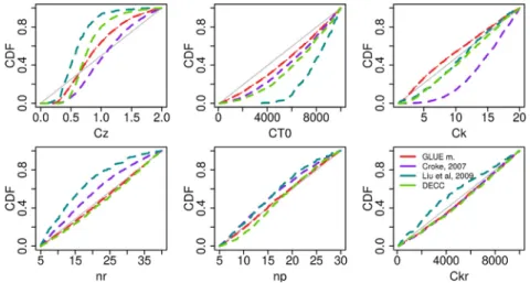
Fig. 3shows the parameter posterior distribution issued from each calibration methodology. Those distributions reflect the first-order sensitivity of parameters to calibration methodology.
All calibration methodologies show that CZand CT0are sensitive
parameters. It reflects how important for model performance are soil properties, both in terms of water storage capacity and sub-surface flow quantification.
With the three calibration methodologies GLUE,Liu et al. (2009)
and DEC, storage capacity of the model is mainly controlled by the CZparameter, the infiltration parameter Ckbeing not sensitive to
calibration. On the opposite, the Croke (2007)method shows a sensitivity to Ck parameter: only high values of Ck results in
behavioural simulations. It seems that the calibration does not have to limit the soil infiltration capacity, as calibration methods either allow or impose high values of infiltration velocity. Finally, all calibration methodologies suggest that runoff production in the MARINE model comes from soil storage capacity exceedence (Dunne, 1978).
The sensitivity of the transmissivity of the soil (CT0parameter)
results from the significant contribution to floods of subsurface flow. The proportion of subsurface flow during high part of hydrographs (^yi>150 m3s$1,Table 2) ranges between 9% and 45%, whatever the calibration method. The similar range of values for the proportion of subsurface flow does not reflect the discrepancies
between posterior distributions of the CT0parameter. Actually, CT0
posterior distributions are correlated with the CZposterior ones.
Discrepancies of CT0posterior distributions seem to compensate
differences between CZposterior distributions producing at the end
a similar volume of subsurface flows.
Looking at the posterior distributions of roughness coefficients, which control surface flow dynamics, only theLiu et al. (2009)and theCroke (2007)methods show sensitivity to the river roughness (nr,Fig. 3). Considering the case of theCroke (2007)method,Fig. 4
shows that the defined error model induces sensitivity to the early rising limb of each event. Indeed, the modelling error interval of the early rising limb obtained without parameter set weighting is huge, and calibration is mainly concerned with minimizing those modelling errors. Finally, the fact that calibration is focused on the early rising limb may explain the sensitivity of the model to river roughness coefficient. Considering theLiu et al. (2009)method, as modelling errors are all valued the same falls outside the confi-dence interval of the observed discharge, their representation does not provide an explanation. Nevertheless, we may suppose, that the small confidence interval around the early rising limb equally makes theLiu et al. (2009)method to enforce accurate prediction for having few modelling errors in this hydrograph part.
The calibration of the last parameter e the coefficient of trans-missivity of the riverbed e results in different posterior distribu-tions betweenLiu et al. (2009)and the three other methodologies. Only theLiu et al. (2009)method shows sensitivity to this param-eter. This sensitivity is not easy to explain as theLiu et al. (2009)
methodology is not focused in any particular hydrological pro-cesses. Nevertheless, it seems that the Ckr parameter has a
compensatory effect on the selection of the other parameters, as correlations between nrand CT0 parameters appear particularly
when calibrating the model with theLiu et al. (2009)methodology. 5.2.2. Hydrograph reproduction comparison
Fig. 5shows the hydrographs of 6 out of 14 flash flood events outputed by the different calibration methods. Observed discharge and corresponding uncertainty are in blue, the median prediction in red and prediction uncertainty in orange. Significant systematic under- (or over-) estimation is visible. Particularly, theCroke (2007)
method tends to underestimate flood discharge, for almost the presented events. On the opposite,Liu et al. (2009)method over-estimates the peak discharge, giving a confidence interval of pre-diction exceeding that of the observed discharge.
Hydrographs show periods when the discharge confidence
Fig. 3. Posterior distributions of parameters after calibration: soil depth Cz;lateral hydraulic conductivity CT0;saturated hydraulic conductivity Ck; and the riverbed and flood plain
Fig. 4. Top window: Hydrographs of 3 selected flash flood events supplied by theCroke (2007)calibration; bottom window: remaining modelling errors along the hydrograph with median prediction in red, and range of modelling errors into the confidence interval of prediction. The grey envelop corresponds to the covered range of modelling errors without any selection of parameter sets. (For interpretation of the references to colour in this figure legend, the reader is referred to the web version of this article.)
Fig. 5. Hydrograph of 6 out of 14 selected flash flood events (for greater clarity) supplied by the different calibration methods: a) GLUE method; b)Croke (2007); c)Liu et al. (2009)method; d) DEC method. Refer toFig. 2for the legend.
interval falls outside the prediction uncertainty whatever the cali-bration method. Those periods could not be simulated properly by the MARINE model. Actually, it emphasizes either the weakness in the model or the input data uncertainty.
5.2.3. Comparison of global performances
Table 3gives the NSE scores successively calculated between the median prediction Y50th and the observed discharge ^Y (line 1); the
lower bound prediction Y5thand the lower bound of the observed
discharge confidence interval ^Y5th(line 2); the upper bound
pre-diction Y95th and the upper bound of the observed discharge
confi-dence interval ^Y95th (line 3). The aim is to assess both the discharge
prediction and the confidence interval of that prediction.
Representation of the observed discharge is similarly reached by the GLUE, DEC andLiu et al. (2009)methodologies, with a NSE score equal to 0,78 and 0,76 respectively.Croke (2007)has the lowest performance with a NSE score equal to 0,63. As said before, the latter method tends to underestimate flood peak (Fig. 5). Similarly, the lower limit of the prediction is underestimated during flow peak with this method and results in the poorest score for the prediction of the lower bound (score ¼ 0,48). Finally, according to the NSE score, the GLUE, theLiu et al. (2009)and the DEC methods show similar results for the median prediction as well as for the interval bounds ones.
Considering another global index for prediction assessment,
Table 4presents the percentage of evaluated points located inside the acceptability zone defined in the DEC definition (equation(11)). The acceptability zone is defined according to user expectations, and consequently appears as the aim of the calibration. The DEC method gives the best percentage with more than 90,26% evaluated points inside the acceptability zone. GLUE method and theLiu et al. (2009) perform similarly with a score of 89,32% and 89,73%, respectively. Regarding the NSE assessment, the Croke (2007)
method gives the lowest result. Considering the prediction for the high parts of the hydrographs (second column,Table 4), the scores give the same range of model performance with best predictions for the DEC method, then in order theLiu et al. (2009)one, the GLUE one, and finally theCroke (2007)one.
Model prediction can alsol be assessed according to water vol-ume flowing at catchment outlet. The bias between predicted and observed discharge reflects the predicted water balance quality. As we know that the model is not accurate for low flow prediction, we calculate the bias only for observed discharge higher than 150 m3s$1(Table 5).
Contrary to the previous metric assessments, calibration methodologies present here very contrasted results.Croke (2007)
underestimates the median prediction and the lower bound pre-diction is far below the interval bound of the observed discharge. It is related to the fact that the method tends to underestimate peak flows as it has been already mentioned when studying hydrograph reproduction (Fig. 5). On the other hand, but not to the same de-gree,Liu et al. (2009)overestimates the median prediction and the lower bound prediction. The most important discrepancy is the
overestimation of the upper bound prediction. Actually, hydro-graph given by the Liu et al. (2009) method shows this over-estimation. It may not appear in the previous score as it represents only a few points during flow peaks, therefore the contribution to the NSE score may not be significant. GLUE presents an over-estimation of the upper bound and an underover-estimation of the lower bound, and consequently gives a larger confidence interval of prediction than the confidence interval of the observed discharge. The confidence interval bandwidth depends on the NSE threshold arbitrarily chosen in order to separate behavioural and non behavioural simulation. The choice of a higher NSE threshold may have decreased the confidence interval bandwidth and therefore resulted in more relevant prediction results.
Overall, only the DEC provides reasonable bias values. Indeed, the median prediction as well as the bound predictions have a bias that does not exceed 18.0 m3s$1, which represents less than 5% of the average of the observed discharge that are higher than 150 m3s$1.
In order to explain the discharge bias discrepancies, we must step back on parameter posterior distribution. Described in x 4,3,1, all calibration methodologies show a model sensitivity to Cz
parameter values, but the resulted posterior distribution of this parameter differs. In particular, calibration methodologies can be ranked according to the median value of Czparameter posterior
distribution.Liu et al. (2009)gives the lower Cz50thfollowed by, DEC,
GLUE and finallyCroke (2007). The selected ranking corresponds to the ranking of bias of the medium prediction, fromLiu et al. (2009)
method showing the highest overestimation, to theCroke (2007)
method presenting the highest underestimation of the median prediction. Actually, it makes sense that the model calibrated with lower depth of storage capacity gives a higher discharge response and inversely.
Moreover, we can notice that posterior distributions of the Cz
parameter from DEC andLiu et al. (2009)reflect a more restricted range of Czvalue, than for the other methods. It may explain that
these methods give smaller confidence interval of prediction around the median discharge prediction.
Finally, most of the discharge bias discrepancies between the different calibration methods may be explained as resulting from Cz, the parameter posterior distribution. The overestimation of the
upper bound prediction during high flows byLiu et al., 2009is not completely clarified. It may result either from the particular cali-bration of the riverbed transmissivity, Ckrwith this method, or from
the selection of smaller values for Cz parameter, that limits soil
storage capacity. Further investigation should be done to confirm it.
6. Conclusion
We presented a calibration method that consistently integrates uncertainty of the discharge observations, model specifics and user-defined tolerance. This is achieved by introducing a new objective function called Discharge Envelop Catching efficiency (DEC). The main idea of the method is enable the end-user to define an acceptability region around the confidence interval of the
Table 4
Percentage of evaluated points of the median prediction inside the acceptability zone defined by in the DEC definition (x 3,2).
Method Percentage of accepted points of the median prediction All points Prediction of points where ^yi>150 m3s$1 DECC 90,26% 76,9%
GLUE 89,32% 74,1% Liu et al., 2009 89,73% 75,7% Croke 2007 87,86% 68,9%
Table 5
Discharge prediction bias on 14 flash flood events when observed discharged is higher than 150 m3s$1. As for NSE calculation, median prediction Y
50
this compared to
the observed discharge ^Y and the predicted bounds (Y5thand Y95th)are compared to the
bounds of the confidence interval of the discharge (^Y5thand ^Y95th).
(m3.s$1) GLUE Croke (2007) Liu et al. (2009) DEC
Median prediction $23 $141 69 5,7 Lower bound prediction $59 $155 55 17,1 Upper bound prediction 149 21 122 15,1
discharge, in relevance with user's expectations. The 90thpercentile of distance distribution from prediction to the acceptability zone is used as the metric score used to assess the model. This score is considered more appropriate than the average of the distribution as it gives priority to the minimization of high distances to the acceptability region.
Using the DEC objective function, a calibration of the MARINE model is tested. The DEC method provides optimal parameter sets since high values of the NSE (0.76) are obtained with the resulting discharge prediction. Also, for 90.11% of the assessment points along the hydrograph, the discharge prediction is enclosed in the acceptability zone. This score is especially conclusive considering that input uncertainty was not taken into account.
We find that the parameter posterior distribution depends on the related calibration method, affirming the role of the objective function. Regarding the impact of the calibration on the modelling error along the hydrograph, it appears that each calibration en-forces the adequacy between observed and predicted discharge at different points or parts of the hydrographs. To be relevant, the assessment of parameter posterior distribution has to be combined with the study of calibration impacts on the hydrographs. Regarding the DEC calibration method, it mainly impacts the pre-diction of flood rising limbs and flow peaks. The resulting param-eter distribution will be most informative for flow processes occurring during the corresponding parts of the hydrographs.
Assessment with the NSE provides similar results from a cali-bration methodology to another, for the median prediction as well as for its confidence interval, although the DEC performs slightly better in average. The flood volume is significantly better predicted when using the DEC method. Likewise, the DEC provides a confi-dence interval for flood volume prediction that is more relevant with respect to the uncertainty of the discharge observations and of the related observed flood volume.
References
Beven, K., 2006. A manifesto for the equifinality thesis. J. Hydrol. 320, 18e36.http:// dx.doi.org/10.1016/j.jhydrol.2005.07.007.
Beven, K., Binley, A., 1992. The future of distributed models: model calibration and uncertainty prediction. Hydrol. Process. 6, 279e298.http://dx.doi.org/10.1002/ hyp.3360060305.
Beven, K., Binley, A., 2014. GLUE: 20 years on. Hydrol. Process. 28, 5897e5918. http://dx.doi.org/10.1002/hyp.10082.
Coxon, G., Freer, J., Westerberg, I.K., Wagener, T., Woods, R., Smith, P.J., 2015. A novel framework for discharge uncertainty quantification applied to 500 UK gauging stations. Water Resour. Res. 51, 5531e5546. http://dx.doi.org/10.1002/ 2014WR016532.
Croke, B., 2007. In: Oxley, Les, Kulasiri, Don (Eds.), The Role of Uncertainty in Design of Objective Functions. International Congress on Modelling and Simulation (MODSIM 2007), vol. 7. Modelling and Simulation Society of Australia and New Zealand Inc., New Zealand, pp. 2541e2547.
Delrieu, G., Wijbrans, A., Boudevillain, B., Faure, D., Bonnifait, L., Kirstetter, P.-E., 2014. Geostatistical radareraingauge merging: a novel method for the quanti-fication of rain estimation accuracy. Adv. Water Resour. 71, 110e124.http://dx. doi.org/10.1016/j.advwatres.2014.06.005.
Dunne, T., 1978. Fiels studies of hillslope flow processes. Hillslope Hydrol. 227e293. Engeland, K., Gottschalk, L., 2002. Bayesian estimation of parameters in a regional hydrological model. Hydrol. Earth Syst. Sci. 6, 883e898. http://dx.doi.org/ 10.5194/hess-6-883-2002.
Garambois, P.A., Roux, H., Larnier, K., Labat, D., Dartus, D., 2015. Parameter regionalization for a process-oriented distributed model dedicated to flash floods. J. Hydrol. 525, 383e399.http://dx.doi.org/10.1016/j.jhydrol.2015.03.052. Gupta, H.V., Kling, H., Yilmaz, K.K., Martinez, G.F., 2009. Decomposition of the mean squared error and NSE performance criteria: implications for improving hy-drological modelling. J. Hydrol. 377, 80e91.http://dx.doi.org/10.1016/j.jhydrol.
2009.08.003.
Habets, F., Boone, A., Champeaux, J.L., Etchevers, P., Franchisteguy, L., Leblois, E., Ledoux, E., Le Moigne, P., Martin, E., Morel, S., 2008. The Safran-Isba-Modcou hydrometeorological model applied over France. J. Geophysical Res.: Atmo-sphere 113, 1984e2012.http://dx.doi.org/10.1029/2007JD008548.
Hornberger, G.M., Spear, R.C., 1981. An approach to the preliminary analysis of environmental systems. J. Environ. Manag. 12 (1), 7e18.
Huard, D., Mailhot, A., 2008. Calibration of hydrological model GR2M using Bayesian uncertainty analysis. Water Resour. Res. 44, W02424. http:// dx.doi.org/10.1029/2007WR005949.
Kavetski, D., Franks, S.W., Kuczera, G., 2003. Confronting input uncertainty in environmental modelling. In: Duan, Q., Gupta, H.V., Sorooshian, S., Rousseau, A.N., Turcotte, R. (Eds.), Calibration of Watershed Models. American Geophysical Union, Washington, D. C..http://dx.doi.org/10.1029/WS006p0049 Kavetski, D., Kuczera, G., Franks, S.W., 2006. Bayesian analysis of input uncertainty
in hydrological modeling: 1. Theory. Water Resour. Res. 42http://dx.doi.org/ 10.1029/2005WR004368.
Kirstetter, P.-E., Delrieu, G., Boudevillain, B., Obled, C., 2010. Toward an error model for radar quantitative precipitation estimation in the C!evenneseVivarais region, France. J. Hydrol. 394, 28e41.http://dx.doi.org/10.1016/j.jhydrol.2010.01.009. Kuczera, G., 1983. Improved parameter inference in catchment models: 1.
Evalu-ating parameter uncertainty. Water Resour. Res. 19, 1151e1162. http:// dx.doi.org/10.1029/WR019i005p01151.
Kuczera, G., Kavetski, D., Franks, S., Thyer, M., 2006. Towards a Bayesian total error analysis of conceptual rainfall-runoff models: characterising model error using storm-dependent parameters. J. Hydrol. 331 (1e2), 161e177.http://dx.doi.org/ 10.1016/j.jhydrol.2006.05.010.
Le Coz, J., Renard, B., Bonnifait, L., Branger, F., Le Boursicaud, R., 2014. Combining hydraulic knowledge and uncertain gaugings in the estimation of hydrometric rating curves: a Bayesian approach. J. Hydrol. 509, 573e587.http://dx.doi.org/ 10.1016/j.jhydrol.2013.11.016.
Liu, Y., Freer, J., Beven, K., Matgen, P., 2009. Towards a limits of acceptability approach to the calibration of hydrological models: extending observation er-ror. J. Hydrol. 367, 93e103.http://dx.doi.org/10.1016/j.jhydrol.2009.01.016. McMillan, H.K., Westerberg, I.K., 2015. Rating curve estimation under epistemic
uncertainty. Hydrol. Process. 29, 1873e1882. http://dx.doi.org/10.1002/ hyp.10419.
Moussa, R., 2010. When monstrosity can be beautiful while normality can be ugly: assessing the performance of event-based flood models. Hydrological Sci. J. 55 (6), 1074e1084.http://dx.doi.org/10.1080/02626667.2010.505893.
Nash, J.E., Sutcliffe, J.V., 1970. River flow forecasting through conceptual models Part I: a discussion of principles. J. Hydrol. 10, 282e290.http://dx.doi.org/10.1016/ 0022-1694(70)90255-6.
Pe~na-Arancibia, J.L., Yongqiang, Z., Pagendam, D.E., Viney, N.R., Lerat, J., van Dijk, A.I.J.M., Vaze, J., Frost, A.J., 2015. Streamflow rating uncertainty: charac-terisation and impacts on model calibration and performance. Environ. Model. Softw. 63, 32e44.http://dx.doi.org/10.1016/j.envsoft.2014.09.011.
Roux, H., Labat, D., Garambois, P.-A., Maubourguet, M.-M., Chorda, J., Dartus, D., 2011. A physically-based parsimonious hydrological model for flash floods in Mediterranean catchments. Nat. Hazards Earth Syst. Sci. 11, 2567e2582.http:// dx.doi.org/10.5194/nhess-11-2567-2011.
Schaefli, B., Gupta, H.V., 2007. Do Nash values have value? Hydrological Process. John Wiley Sons, Ltd. 21, 2075e2080.http://dx.doi.org/10.1002/hyp.6825. Schaefli, B., Hingray, B., Niggli, M., Musy, A., 2005. A conceptual glacio-hydrological
model for high mountainous catchments. Hydrol. Earth Syst. Sci. 9, 95e109. http://dx.doi.org/10.5194/hess-9-95-2005.
Schoups, G., Vrugt, J.A., 2010. A formal likelihood function for parameter and pre-dictive inference of hydrologic models with correlated, heteroscedastic, and non-Gaussian errors. Water Resour. Res. 46 http://dx.doi.org/10.1029/ 2009WR008933.
Seibert, J., 2001. On the need for benchmarks in hydrological modelling. Hydro-logical Process. John Wiley Sons, Ltd. 15, 1063e1064.http://dx.doi.org/10.1002/ hyp.446.
Tabary, P., 2007. The new French operational radar rainfall product. Part I: meth-odology. Weather Forecast. 22, 393e408.http://dx.doi.org/10.1175/WAF1004.1. Thyer, M., Renard, B., Kavetski, D., Kuczera, G., Franks, S.W., Srikanthan, S., 2009. Critical evaluation of parameter consistency and predictive uncertainty in hy-drological modeling: a case study using Bayesian total error analysis. Water Resour. Res. 45, W00B14.http://dx.doi.org/10.1029/2008WR006825. Villarini, G., Krajewski, W., 2010. Review of the different sources of uncertainty in
single polarization radar-based estimates of rainfall. Surv. Geophys. 31, 100e129.http://dx.doi.org/10.1007/s10712-009-9079-x.
Vrugt, J.A., Sadegh, M., 2013. Toward diagnostic model calibration and evaluation: approximate Bayesian computation. Water Resour. Res. 49, 4335e4345.http:// dx.doi.org/10.1002/wrcr.20354.