M
AN
US
CR
IP
T
AC
CE
PT
ED
1 MANUSCRIPT 2 3A guideline to select an estimation model of daily global solar radiation between
4geostatistical interpolation and stochastic simulation approaches
56
7
D. I. Jeong1), A. St-Hilaire2), Y. Gratton2), C. Bélanger2), C. Saad3)
8
1
Centre ESCER (Étude et Simulation du Climat à l’Échelle Régionale), Université du Québec
9
à Montréal, Montreal, Canada
10
2
INRS-ETE, University of Québec, Québec, Canada
11
3
Environment and Climate Change Canada, Montreal, Canada
12 13 14 15 16 17 18 19
Corresponding author address: Dae Il Jeong, Ph.D., P.Eng., Centre ESCER, Université du 20
Québec à Montréal, 201 Ave. President-Kennedy, Montreal, Quebec H3C 3P8, Canada
21
Email: jeong@sca.uqam.ca
M
AN
US
CR
IP
T
AC
CE
PT
ED
Abstract 23This study compares geostatistical interpolation and stochastic simulation approaches for the
24
estimation of daily global solar radiation (GSR) on a horizontal surface in order to fill in
25
missing values and to extend short record length of a meteorological station. A guideline to
26
select an approach is suggested based on this comparison. Three geostatistical interpolation
27
models are developed using the nearest neighbor (NN), inverse distance weighted (IDW), and
28
ordinary kriging (OK) schemes. Three stochastic simulation models are also developed using
29
the artificial neural network (ANN) method with daily temperature (ANN(T)), relative
30
humidity (ANN(H)), and both (ANN(TH)) variables as predictors. The six models are
31
compared at 13 meteorological stations located across southern Quebec, Canada. The three
32
geostatistical interpolation models yield better performances at stations located in a high
33
density area of GSR measuring stations compared to the three stochastic simulation models.
34
The guideline suggests an optimal approach by comparing a threshold distance, estimated
35
according to a performance criteria of a stochastic simulation model, to the distance between a
36
target and its nearest neighboring station. Additionally, the spatial correlation strength of daily
37
GSRs and the at-site correlation strength between daily GSRs and the predictor variables
38
should be considered.
39
40
Keywords: artificial neural networks, geostatistical interpolation, global solar radiation, spatial 41
correlation, temperature, relative humidity.
M
AN
US
CR
IP
T
AC
CE
PT
ED
1. Introduction 43Global solar radiation (GSR) on a horizontal surface of the earth is an important variable for
44
many analyses involving agricultural and plant growth, air and water temperatures,
45
environmental and biological risk, and solar electric generation. However, instruments
46
measuring solar irradiation (i.e., Kipp or Eppley pyranometers) are relatively expensive and
47
difficult to manage [1], compared to those of common meteorological variables such as air
48
temperature, precipitation, and relative humidity. Therefore, meteorological stations for GSR
49
are generally less abundant than those for the common meteorological variables. Furthermore,
50
observed GSR datasets are usually short timeseries and have large gaps of missing values.
51
Geostatistical interpolation approaches can be adopted to fill in missing values and to
52
extend short record length of the GSR at a station using observed GSR data on the other
53
stations located near the desired station. Kriging [2-7], nearest neighbor [4], and inverse
54
distance weighted average [5,8,9] approaches have been applied frequently for the spatial
55
interpolation.
56
At-site physical and statistical approaches can also be used for GSR simulations.
57
Physical models (e.g., [10-12]) use complex physical interactions between the GSR and the
58
terrestrial atmosphere, such as the Rayleigh scattering, radiative absorption by ozone and
59
water vapour and aerosol extinction. Stochastic simulation models (e.g., [13-20]) use
60
empirical relationships between GSR and meteorological covariables such as sunshine hours,
61
temperature, and relative humidity at a desired station. This study considers stochastic
62
simulation models as they are relatively simple to develop and require fewer input variables
63
compared to physical models [16,17]. Although linear and non-linear regressions as well as
64
artificial neural networks (ANNs) can be employed to drive empirical relationships between
65
the common meteorological variables and the GSR, many studies [16-18,20-22] have shown
M
AN
US
CR
IP
T
AC
CE
PT
ED
the superiority of ANN approaches to regression-based approaches.
67
Sunshine duration, one of the most explanatory variables for GSR simulation
68
[18,21,23], has not been recorded at most meteorological stations in Canada since 1999 due to
69
its difficulty of measurement [1]. Temperature [13-15,17-19,24-28] and relative humidity
70
[18,21] are alternative covariables although they have weaker correlation with GSR compared
71
to sunshine duration [18].
72
Geostatistical interpolation and statistical simulation approaches for GSR estimation
73
have been applied separately in many studies, however, they have been rarely compared in an
74
application study. Therefore, this study compares geostatistical interpolation and statistical
75
simulation approaches to fill in missing values and to extend short record length of daily GSR
76
timeseries. The spatial interpolation approaches considered include the nearest neighbor, the
77
inverse distance weighted, and the ordinary kriging methods. The stochastic simulation
78
models include three ANN-based models with daily temperature and/or daily relative
79
humidity as input variables. The six models are applied at 13 meteorological stations located
80
across southern Quebec (45.1~50.3 °N and 64.2~79.0 °W), Canada. Furthermore, a guideline
81
to choose an approach between the geostatistical interpolation and the statistical simulation
82
approaches is provided for the estimation of daily GSR on the study area.
83
84
2. Methodologies
85
2.1 Geostatistical interpolation models
86
Three geostatistical interpolation models are developed based on nearest neighbor (NN),
87
inverse distance weighted (IDW), and ordinary kriging (OK) schemes for daily GSR. The NN
88
model employs the simplest algorithm among the three models. This model selects the value
89
of the nearest station to the location of interest and does not consider the other values of
M
AN
US
CR
IP
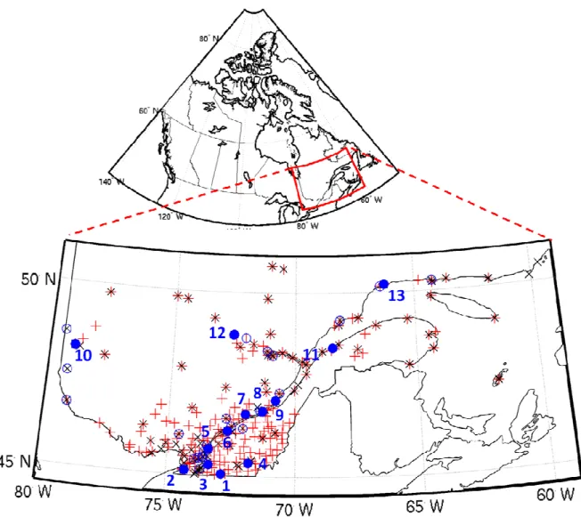
T
AC
CE
PT
ED
neighboring stations in order to yield a piecewise-constant interpolation map.
91
The IDW interpolation algorithm adopts the assumption that the interpolation value at
92
a location of interest is inversely proportional to the distances of nearby stations. The
93
interpolation value of the model is a weighted average of the values of multiple stations and
94
the weight assigned to each nearby station diminishes as the distance from the interpolation
95
point to that station increases. The IDW model interpolates the daily GSR value R(x0) at an
96
ungauged location x0 from observations R(xi) at locations x ...,1, xn as follows:
97 98
∑
= = n i i iR x w x R 1 0) ( ) ( ˆ (1) 99∑
= = n j j i i d d w 1 / 1 / 1 , i=1,2,...,n (2) 100 101where Rˆ(x0) is an interpolated value of R(x0) and di represents distance between R(x0)
102
and R(xi).
103
Kriging is a geostatistical interpolation technique based on the linear least square
104
estimation algorithm. Ordinary kriging (OK) is the most common among many kriging
105
approaches. OK estimates the best linear unbiased estimator based on a linear model. The
106
interpolation value of the OK at a location x0 is given by the following equation:
107 108 = ) ( ) ( ) ( ˆ 1 T ' 1 0 n n R x x R w w x R M M (3) 109
M
AN
US
CR
IP
T
AC
CE
PT
ED
110where w ...,1, wn are the weights of the OK that fulfill the unbiased condition
∑
= = n i i w 1 1 . The 111
weights are obtained by the below OK equation system:
112 113 = − 1 ) , ( ) , ( 0 1 1 1 ) , ( ) , ( 1 ) , ( ) , ( 0 0 1 1 1 1 1 1 1 x x x x x x x x x x x x w w n n n n n n
γ
γ
γ
γ
γ
γ
µ
M L K M M O M L M (4) 114 115where µ =E[R(x)] is a Lagrange parameter employed to minimize the kriging error under
116
the unbias condition, which is assumed to be an unknown constant in the OK. γ(xi,xj) is a
117
variogram function to calculate the spatial dependency between R(xi) and R(xj). Several
118
variogram functions are available such as exponential, Gaussian, and spherical models. In this
119
study, the spherical variogram function is selected based on trial and error examination. The
120
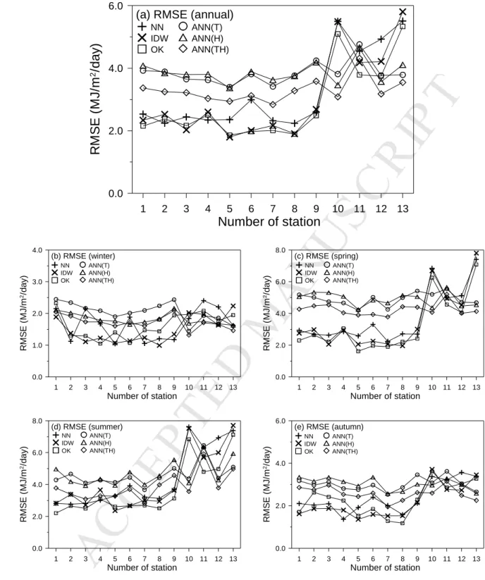
variogram is estimated for each day, based on observed daily GSR dataset of nearby stations.
121
The detail descriptions of variogram models and ordinary kriging can be found in [29,30].
122
To verify the interpolation performances of the three models, a leave-one-out
cross-123
validation approach is employed. Among the observations at n stations, GSR values of one of
124
those stations are interpolated using the observations at the remaining n-1 stations. This
125
process is repeated for all the observation stations. The interpolated Rˆ(xi) is then compared
126
to the associated observation R(xi) at each station in order to evaluate the performance of
127
the interpolation models.
128
2.2 Stochastic simulation models
M
AN
US
CR
IP
T
AC
CE
PT
ED
Three stochastic simulation models are developed to estimate daily GSR using the ANN
130
approach as a transfer function and daily maximum and minimum temperatures and/or daily
131
mean relative humidity as input variables. Feed forward ANNs have been frequently
132
employed to simulate GSR [16-18, 20, 21] from the meteorological input variables. This
133
study also employs a three-layer feed forward ANN model, which includes an input layer, a
134
single hidden layer, and an output layer of computation nodes. The ANN models are trained
135
by the Bayesian regularization backpropagation (BRBP) algorithm, which is a network
136
training function that updates the weight and bias values according to the
Levenberg-137
Marquardt optimization [31]. An important issue in ANN modelling is the determination of
138
the number of hidden nodes. Fletcher and Goss [32] suggested that the optimal number of
139
hidden nodes could be within (2p0.5+ o) ~ (2p+1), where p and o are the numbers of
140
independent and dependent variables, respectively. The hyperbolic tangent sigmoid function
141
is employed for the hidden layer and the linear function is used for the output layer. Detailed
142
descriptions of these various activation functions are provided in [31]. The three ANN models
143
used to simulate daily GSR series from daily meteorological variables are as follows:
144 145 ) , , ( ˆ min max T Ra T ANN R= (5) 146 ) , ( ˆ a R H ANN R= (6) 147 ) , , , ( ˆ min max T H Ra T ANN R= (7) 148 149
where Tmax and Tmin are daily maximum and minimum temperatures (°K) and H is daily
150
mean relative humidity in a given day. The ANN represents the three-layer feed forward
151
ANN trained by the BRBP algorithm. The Ra is the solar irradiation on a horizontal surface
M
AN
US
CR
IP
T
AC
CE
PT
ED
at the top of the atmosphere, which is a function of latitude and Julian day of a site. It is
153
calculated by using the standard geometric method provided by [33]. The details of the
154
method are also available in [20]. The three models are called ANN(T), ANN(H), and
155
ANN(TH) hereafter based on employed input variables. The numbers of hidden nodes
156
selected for the ANN(T), ANN(H), and ANN(TH) are 4, 3, and 5, respectively, based on a
157
trial-and-error procedure.
158
Daily GSR at ungauged stations that measure other predictor variables can be
159
simulated using a regional ANN-based model. This model is calibrated based on all available
160
GSR and meteorological observations for the region of interest, which allows for the
161
simulation of GSR at ungauged stations where covariables are available. For instance, Fortin
162
et al. [17] and Jeong et al. [20] tested a regional ANN-based model to simulate daily GSR for
163
regional areas located in eastern Canada. They calibrated this model using observations
164
obtained from a set of stations and validated the model using those obtained from a different
165
station set. Regional ANN(T), ANN(H), and ANN(TH) models are also considered in this
166
study using a leave-one-out training procedure. In this approach, the regional ANN models
167
are trained for a given station using observations of all the remaining stations for the
168
calibration period, which is repeated for all stations. In the regional ANN models, mean GSR
169
varies according to Ra, which is a function of the latitude of each station.
170
171
2.3 Model evaluation measures
172
Simulation performances are evaluated using the mean bias error (MBE), root mean square
173
error (RMSE), and R-square (coefficient of determination). The MBE and RMSE are given by
174
the following equations:
M
AN
US
CR
IP
T
AC
CE
PT
ED
176∑
= − = m i i i R R m 1 ) ˆ ( 1 MBE (8) 177∑
= − = m i i i R R m 1 5 . 0 2 ] ) ˆ ( 1 [ RMSE (9) 178 179where Ri and Rˆ are observed and simulated daily GSR values and m is the record length. i
180
R-square (coefficient of determination) is the squared value of the (Pearson’s
product-181
moment) linear correlation coefficient between observed and simulated values. It can provide
182
the proportion of explained variance of observations by an applied model and is defined by
183
the following equation:
184 185
∑
∑
= = − − − = m i i m i i i R R R R 1 2 1 2 2 ) ( ) ˆ ( 1 r (10) 186 187where R is the mean of the observed GSR values.
188
189
3. Study area and data
190
Daily GSR, maximum and minimum temperatures, as well as mean relative humidity are
191
obtained from 13 meteorological stations of Environment Canada (EC) located between
192
latitude 45.1°N to 50.3°N and longitude 64.2°W to 79.0°W (i.e. Southern Quebec, Canada).
193
The daily GSR and the two predictor variables are obtained for the analysis period from 2003
194
to 2010. Figure 1 shows the locations of the 13 stations across southern Quebec, which have
M
AN
US
CR
IP
T
AC
CE
PT
ED
less than 10 % of missing data of daily maximum and minimum temperatures, relative
196
humidity, and GSR for the analysis period. The figure also distinguishes the GSR stations
197
excluded from this analysis due to more than 10 % of missing values of any of the three
198
previously mentioned variables. Stations recording daily maximum and minimum
199
temperatures and relative humidity are presented when they have less than 50 % of missing
200
data for the analysis period. The south of Quebec is the most populated and productive area in
201
the province and has higher density of observation stations than the rest of the province. The
202
three stochastic simulation models are calibrated and validated on the 2003-2007 and
2008-203
2010 periods, respectively. The three geostatistical interpolation models interpolate the daily
204
GSR for each observation station by using the leave-one-out cross-validation method for the
205
2008-2010 period. Performances of the six models are finally compared for the 2008-2010
206
validation period at the 13 selected stations.
207
Table 1 presents the information (station identification numbers, latitudes, longitudes,
208
and altitudes) of the 13 stations in ascending order of their latitudes. Annual and seasonal (i.e.,
209
DJF for winter, MAM for spring, JJA for summer, and SON for autumn) averages of daily
210
GSR for the 2003-2010 period are also provided. In general, it is known that GSR decreases
211
as latitudes increase; however, the annual or seasonal GSR of the stations do not show a clear
212
decrease as their latitudes increase because the study area covers a small range of latitude (5.2
213
degree). Furthermore, some stations are located in complex climate conditions directly
214
affected by the St-Lawrence River and convections from the Atlantic Ocean (i.e., stations 8, 9,
215
11, and 13) or from the continent (i.e., station 10). As daily GSR and predictor variables are
216
not linearly correlated, linear correlation coefficients between the solar transmissivity (i.e., the
217
ratio of incoming GSR on the surface of the earth to solar irradiation at the top of the
218
atmosphere) and diurnal temperature range (DTR; Tmax - Tmin)
γ
(R/Ra,DTR) series as wellM
AN
US
CR
IP
T
AC
CE
PT
ED
as between solar transmissivity and daily mean relative humidity
γ
(R/Ra,H) series are220
presented. The solar transmissivity and DTR have positive correlations since a cloudy day has
221
smaller GSR, and also a smaller DTR due to a lower Tmax during the day by blocking sunlight
222
as well as a higher Tmin during the night by preventing radiative cooling, when compared to a
223
clear day. However, the solar transmissivity and mean daily relative humidity are negatively
224
correlated since a clear day has less humidity than a cloudy day. Correlations between daily
225
GSR and DTR and relative humidity of station 11 are weaker than those of the other stations.
226
This station is located on the south shore of the Lower St-Lawrence valley, which has
227
complex climate conditions affected by the river and convections from the continent and the
228 Atlantic Ocean. 229 230 4. Results 231
4.1 Comparison of model performances
232
Table 2 presents performance measures of the geostatistical interpolation models for each
233
station for the 2008-2010 validation period. The NN, which is the simplest approach, yields
234
the worst performance, whereas the OK, which is the most sophisticated approach, shows the
235
best performance, although there is a larger magnitude of MBE for OK than for IDW. The
236
three models generally produce larger MBE at stations 10, 12, and 13, which have larger
237
differences in annual mean GSR values compared to the other stations (see Table 1 for values
238
of annual mean GSR and Figure 1 for station locations). The three models yield small RMSEs
239
at stations located in the high density area (i.e., stations 1 to 9), whereas they yield large
240
RMSEs at stations located in the low density area (i.e., stations 10 to 13). In this low density
241
area, the nearest stations to the stations 10-13 are located within a distance of 482.0, 235.2,
242
236.1, and 363.8 km, respectively, whereas those to the stations 1-9 are located within 100 km.
M
AN
US
CR
IP
T
AC
CE
PT
ED
It is notable that the performance of the geostatistical interpolation models depends on the
244
density of the network of stations and on the statistical homogeneity of GSR values.
245
Table 3 presents performances of the stochastic simulation models for each station for
246
the calibration and validation periods. The differences of the performances between the
247
calibration and the validation periods are modest for each model and for each station,
248
implying that the three models are calibrated well without overfitting and that they have good
249
generalization ability for a new data set. Average differences between the two periods are 0.35
250
MJ/m2/day for MBE, 0.20 MJ/m2/day for RMSE, and 1.8 % for R-square. Among the three
251
stochastic simulation models, the ANN(TH) uses both temperature and relative humidity as
252
input variables and yields the best performance. The ANN(T) and the ANN(H), which employ
253
either temperature or relative humidity as an input variable, yield similar performances for all
254
stations, except for the station 11, which showed the weakest correlations between daily GSR
255
and predictors among the selected stations (Table 1).
256
Figure 2 compares RMSEs of the geostatistical interpolation and the stochastic
257
simulation models for each station at annual and seasonal scales for the validation period. The
258
geostatistical interpolation models generally show better performance than the stochastic
259
simulation models for the stations located in the high density area (i.e., stations 1 to 9).
260
However, these models perform differently for the stations located in the low density area (i.e.,
261
stations 10 to 13). The poor performances of the geostatistical interpolation models in the low
262
density area are expectable as the models use spatial correlations, which exponentially
263
decrease as distance increase. Especially in spring and summer, RMSEs of the geostatistical
264
models tend to be larger at stations 10, 12, and 13 than the stochastic simulation models,
265
indicating that spatial correlation structures of GSR are weaker in spring and summer than in
266
winter and autumn. However, the stochastic simulation models have similar performances for
M
AN
US
CR
IP
T
AC
CE
PT
ED
all stations, except for the station 11, as they only use at-site relationship between the daily
268
GSR and the input variables.
269
Figure 3 presents scatter plots between observed and simulated daily GSRs for the
270
validation period and for stations 7 and 13, which are located in the high density and the low
271
density (i.e., north-eastern boundary) areas, respectively. In Figures 3a to 3f, the geostatistical
272
interpolation models show better agreement with the 1:1 line than the stochastic simulation
273
models at the station 7. As shown in Tables 2 and 3, the OK model yields the best
274
performance among the six models at this station. However, the geostatistical interpolation
275
models tend to overestimate the observed values at the station because, on average, daily
276
GSRs at the station are smaller than its neighboring stations (see Table 1). In Figures 3g to 3l,
277
the geostatistical interpolation models show worse agreement with the 1:1 line than the
278
stochastic simulation models at the station 13. The ANN(TH) model yields the best
279
performance among the six models.
280
4.2 Guidelines for model selection
281
RMSEs and R-squares of daily GSR series between a target and a neighboring station versus
282
their distance for all possible pairs of stations are presented in Figure 4, at an annual and
283
seasonal scales for the 2003-2010 period. In other words, the RMSEs and R-squares of the
284
NN method are calculated, under the assumption that the pair of stations includes the target
285
station and its nearest neighbor. Trend lines of RMSEs and R-squares are estimated by the
286
logarithmic and exponential functions respectively using the non linear least square algorithm.
287
Equations and R-squares of the trend lines for annual and season scales are provided in the
288
figures. Therefore, the trend lines provide approximate RMSEs or R-squares of the NN
289
method for a target station with its nearest neighbor on the study area. For instance, according
290
to the equation presented in Figure 4a, if an observed daily GSR value is available at the
M
AN
US
CR
IP
T
AC
CE
PT
ED
nearest neighboring station located at a distance of 200km from a target station, the NN
292
method can approximately simulate the daily GSR at the target station with an expected
293
RMSE of 4.3 MJ/m2/day at an annual scale. Spatial correlation strengths vary between
294
seasons. For instance, in winter and autumn, the spatial correlation structures are stronger than
295
those in spring and summer. The study area usually shows more homogenized weather and
296
solar radiation conditions in winter and autumn compared to spring and summer seasons
297
because of less convection from Atlantic and/or continental sources.
298
Using the equations presented in Figure 4, a threshold distance (TD) between a target
299
and its nearest neighboring station can be estimated according to a desired level of
300
performance (i.e., RMSE or R-square) based on the NN model. In Table 4, estimated TDs of
301
the NN model are presented based on the RMSEs of each ANN(T), ANN(H), and ANN(TH)
302
models presented in Table 3. Based on the table, worse performances of the NN models are
303
expected than the stochastic simulation models at stations 10, 12, and 13 as their nearest
304
neighboring stations are located further than their TDs. Similarly, the NN model can yield
305
slightly better performance than ANN(T) and ANN(H), but it can yield a worse performance
306
than ANN(TH) annually at station 11. This can be explained by the NN model requiring
307
nearest neighboring stations to be within 263 km for ANN(T), 245 km for ANN(H), and 212
308
km for ANN(TH) at an annual scale, but the nearest station (i.e., station 9) is actually at a
309
distance of 235.2 km from station 11.
310
The TDs presented in Table 4 can be used as a guideline to select an approach
311
between geostatistical interpolation and stochastic simulation models by comparing estimated
312
TDs to the distances of the nearest neighboring stations when filling in missing values and
313
extending record length of daily GSR is required at an observation station. There are three
314
possible cases; (1) TD > distance of nearest neighboring station; (2) TD ≈ distance of nearest
M
AN
US
CR
IP
T
AC
CE
PT
ED
neighboring station; (3) TD < distance of nearest neighboring station. For the first case,
316
applying the geostatistical interpolation models is recommended. For instance, on average,
317
better annual performances of the NN model can be expected than the ANN(T), ANN(H), and
318
ANN(TH) when a nearest neighboring station is within 162, 164, and 121 km, respectively.
319
However, the availability of predictor variables (i.e., temperature and/or humidity) of
320
statistical simulation models and the seasonal spatial correlation strengths of geostatisical
321
interpolation models should be considered to select an optimal approach. As ANN(TH) yields
322
better performance than ANN(T) or ANN(H), the former's TD is shorter than the latter's.
323
Shorter TDs are estimated in summer compared to the winter and autumn seasons due to a
324
weak spatial correlation structure in summer. In the second case, applying more sophisticated
325
geostatistical interpolation models (e.g., IDW and OK) than the NN model is recommended.
326
As an example, at station 7, the IDW and OK models yield better performances, whereas the
327
NN model yield a worse performance compared to the ANN(TH) annually (see Figure 3a).
328
Finally, in the third case, applying stochastic simulation models is recommended as they
329
generally can perform better than geostatistical interpolation models. Since the best
330
performance model cannot always be applied for a specific period at a selected station due to
331
a lack of available predictor variables and observed GSR values of neighboring stations, the
332
TD criterion of the proposed guideline can be used to suggest an optimal approach. The
333
guideline and TD can also be used for other GSR stations that were excluded in this analysis
334
due to short record-length (Figure 1).
335
Under the assumption that a target station has only predictor variables, regional
336
stochastic simulation models are developed using the GSR and predictor variables measured
337
at the other stations. Table 5 presents annual performances of regional models for the 13
338
stations and their TDs to the nearest neighboring stations to produce similar RMSEs to the
M
AN
US
CR
IP
T
AC
CE
PT
ED
regional models. Among the regional ANNs, ANN(TH) yields the best performance while
340
regional ANN(T) and ANN(H) yield similar performances to each other. Again, station 11
341
shows the worst performance among the 13 stations. The RMSEs of the regional models are
342
0.21~0.27 MJ/m2/day larger than those of the at-site models. The worse performances of
343
regional ANNs are reasonable compared to the at-site ANNs as the regional ANNs at each site
344
do not use the observed GSR data of that site for the model calibrations. Consequently, the
345
TDs of the regional models are also 14.9~29.1 km longer than those of the at-site models.
346
These TD values and the ones presented in Table 5 can thus be used to select an appropriate
347
approach between geostatistical interpolation and regional ANN simulation approaches in
348
order to estimate daily GSR at ungauged (or short-record) stations.
349
350
5. Concluding remarks
351
Geostatistical interpolation and stochastic simulation approaches are compared in this study to
352
fill in missing values and to extend short record length of the daily global solar radiation
353
(GSR). However, it is notable that the comparison is only based on the performances of two
354
approaches because they have different application constraints and algorithms to each other.
355
For instance, geostatistical interpolation approaches provide interpolated values at any point
356
in a region including a target station; however, they need observations of daily GSR on the
357
other stations located near the target station to estimate the spatial correlation structure.
358
Stochastic simulation approaches provide estimated values only at the target station using
359
observed daily GSR series as a dependant variable, and daily temperatures as well as
360
humidity series as independent variables.
361
The simplest nearest neighbor (NN) model yields the worst performance, whereas the
362
most sophisticated ordinary kriging (OK) model shows the best performance among the three
M
AN
US
CR
IP
T
AC
CE
PT
ED
geostatistical interpolation models. The three geostatistical interpolation models generally
364
yield smaller RMSEs at stations located in the high density area (i.e., stations 1-9) than those
365
located in the low density area (i.e., stations 10-13). The difference of the performances of
366
geostatistical interpolation models between the high and low density areas can be explained
367
by the exponential decrease of the spatial correlations between stations as the distance
368
increase. Among the three at-site stochastic simulation approach models, the ANN(TH) yields
369
better performance than the ANN(T) and ANN(H), while the ANN(T) and ANN(H) yield
370
similar performances to each other. The three stochastic simulation models produce similar
371
performances for all stations, except for the station 11, which is exposed to a complex climate
372
and showed weaker relationships between GSR and predictors. Regional stochastic simulation
373
models can simulate daily GSR series at stations, where only predictor variables are available;
374
however, the performances of the regionalized models are worse than the at-site models.
375
In the comparison between the geostatistical interpolation and the stochastic
376
simulation models, the geostatistical models perform better at stations located in the high
377
density area, but they perform worse at stations located in the low density area, compared to
378
the stochastic simulation models. Equations that can approximately estimate the RMSE and
379
R-square based on the NN model using the distance between a target and its nearest
380
neighboring station are presented. By using these equations, a guideline is suggested to select
381
an approach between the geostatistical interpolation and the stochastic simulation approaches.
382
A stochastic simulation approach is recommended when the distance between a target and its
383
nearest neighboring station is longer than the threshold distance (TD) estimated according to
384
the RMSE of a stochastic simulation model. In the opposite case, when the TD is longer than
385
the distance between a target and its nearest neighboring station, a geostatistical interpolation
386
approach is recommended. When the TD is similar to the distance between a target and its
M
AN
US
CR
IP
T
AC
CE
PT
ED
nearest neighboring station, more sophisticated geostatistical interpolation models (e.g., IDW
388
and OK) have generally proven to perform better than a stochastic simulation model in this
389
study.
390
Although, this study suggests a guideline to select an appropriate simulation approach
391
for daily GSR between geostatistical interpolation and stochastic simulation approaches, the
392
guideline is dependent on the spatial correlation strength of daily GSRs and the at-site
393
correlation strength between daily GSRs and the predictor variables. It is proved that spatial
394
correlation strengths for seasonal scales have stronger in winter and autumn compared to
395
those in spring and summer in the study area. Simulation of sub-daily GSR will be considered
396
in future work as it is generally more important than daily GSR to estimate solar energy
397
output due to the non-linear relationship between the radiance and the energy output.
398
399
Acknowledgements
400
This study was financed by a team grant from Ouranos to Yves Gratton, André St-Hilaire,
401
Isabelle Laurion, and J.-C Auclair and by NSERC Discovery grants to André St-Hilaire,
402
Isabelle Laurion, and Yves Gratton. We would like to thank David Huard from Ouranos for
403
his help.
404
M
AN
US
CR
IP
T
AC
CE
PT
ED
References 406[1] H.W. Cutforth, D. Judiesch, Long-term changes to incoming solar energy on the
407
Canadian Prairie, Agricultural and Forest Meteorology 145 (2007) 167-175.
408
[2] S. Rehman, S.G. Ghori, Spatial estimation of global solar radiation using geostatistics,
409
Renewable Energy 21 (2000) 583-605.
410
[3] G.G. Merino, D. Jones, D.E. Stooksbury, K.G. Hubbard, Determination of
411
semivariogram models to krige hourly and daily solar irradiance in western Nebrask,
412
Journal of applied meteorology 40 (2001) 1085-1094.
413
[4] J. Mubiru, K. Karume, M. Majaliwa, E.J.K.B. Banda, T. Otiti, Interpolating methods for
414
solar radiation in Uganda, Theoretical and Applied Climatology 88 (2007) 259-263.
415
[5] H. Apaydin, F.K. Sonmez, Y.E. Yildirim, Spatial interpolation techniques for climate
416
data in the GAP region in Turkey, Climate Research 28 (2004) 31-40.
417
[6] H. Alsamamra, J.A. Ruiz-Arias, D. Pozo-Vázquez, J. Tovar-Pescador, A comparative
418
study of ordinary and residual kriging techniques for mapping global solar radiation
419
over southern Spain, Agricultural and Forest Meteorology 149 (2009) 1343-1357.
420
[7] J.A. Ruiz-Arias, D. Pozo-Vázquez, F.J. Santos-Alamillos, V. Lara-Fanego, J.
Tovar-421
Pescador, A topographic geostatistical approach for mapping monthly mean values of
422
daily global solar radiation: A case study in southern Spain, Agricultural and Forest
423
Meteorology 151 (2011) 1812– 1822.
424
[8] Zelenka, G. Czeplak, V. D’Agostino, J. Weine, E. Maxwell, R. Perez, Techniques for
425
supplementing solar radiation network data, In Report IEA Task 9, Vol. 2, Report No.
426
IEA-SHCP-9D-1, 1992.
427
[9] C.L. Goodale, J.D. Aber, S.V. Ollinger, Mapping monthly precipitation, temperature,
428
and solar radiation for Ireland with polynomial regression and a digital elevation model,
M
AN
US
CR
IP
T
AC
CE
PT
ED
Climate Research 10 (1998) 35-49. 430[10] D. Leckner, The spectral distribution of solar radiation at the earth’s surface-elements of
431
a model, Solar Energy 20 (1978) 143-150.
432
[11] De La Casiniere, A.I. Bokoye, T. Cabot, Direct solar spectral irradiance measurements
433
and updated simple transmittance models, Journal of Applied Meteorology 36 (1997)
434
509-520.
435
[12] Gueymard, A two-band model for the calculation of clear sky solar irradiance,
436
illuminance and photosynthetically active radiation at the earth’s surface, Solar Energy
437
43 (1989) 253-265.
438
[13] R. Mahmood, K.G. Hubbard, Effect of time of temperature observation and estimation
439
of daily solar radiation for the northern Great Plains, USA, Agronomy Journal 94 (2002)
440
723-733.
441
[14] Weiss, C. Hays, Simulation of daily solar irradiance, Agricultural and Forest
442
Meteorology 123 (2004) 187-199.
443
[15] M. Trnka, Z. Žalud, J. Eitzinger, M. Dubrovský, Global solar radiation in Central
444
European lowlands estimated by various emprical formulare, Agricultural and Forest
445
Meteorology 131 (2005) 54-76.
446
[16] F.S. Tymvios, C.P. Jacovides, S.C. Michaelides, C. Scouteli, Comparative study of
447
Angstrom's and artificial neural networks' methodologies in estimating global solar
448
radiation, Solar Energy 78 (2005) 752-762.
449
[17] J.G. Fortin, F. Anctil, L.E. Parent, M.A. Bolinder, Comparison of empirical daily surface
450
incoming solar radiation models, Agricultural and Forest Meteorology 148 (2008)
1332-451
1340.
452
[18] M. Benghanem, A. Mellit, S.N. Alamri, ANN-based modelling and estimation of daily
M
AN
US
CR
IP
T
AC
CE
PT
ED
global solar radiation data: A case study, Energy Conversion and Management 50
454
(2009) 1644-1655.
455
[19] X. Liu, X. Mei, Y. Li, Q. Wang, J.R. Jensen, Y. Zhang, J.R. Porter, Evaluation of
456
temperature-based global solar radiation models in China, Agricultural and Forest
457
Meteorology 149 (2009) 1433-1446.
458
[20] D.I. Jeong, A. St-Hilaire, Y. Gratton, C. Bélanger, C. Saad, Simulation and
459
Regionalization of Daily Global Solar Radiation: A Case Study in Quebec, Canada,
460
Atmosphere-Ocean 54 (2016) 117-130.
461
[21] J. Mubiru, E.J.K.B. Banda, Estimation of monthly average daily global solar irradiation
462
using artificial neural networks, Solar Energy 82 (2008) 181-187.
463
[22] Y. Jiang, Prediction of monthly mean daily diffuse solar radiation using artificial neural
464
networks and comparison with other empirical models, Energy Policy 36 (2008)
3833-465
3837.
466
[23] M.A. Behrang, E. Assareh, A.R. Noghrehabadi, A. Ghanbarzadeh, New sunshine-based
467
models for predicting global solar radiation using PSO (particle swarm optimization)
468
technique, Energy 36 (2011) 3036-3049.
469
[24] K.L. Bristow, G.S. Campbell, On the relationship between incoming solar radiation and
470
daily maximum and minimum temperature, Agric. For. Meteolo. 31 (1984) 159-166.
471
[25] R. De Jong, D.W. Stewart, Estimating Global Solar-Radiation from Common
472
Meteorological Observations in Western Canada, Canadian Journal of Plant Science 73
473
(1993) 509-518.
474
[26] G.P. Podestá, L. Núñez, C.A. Villanueva, M.A. Skansi, Estimating daily solar radiation
475
in the Argentine Pampas, Agricultural and Forest Meteorology 123 (2004) 41-53.
476
[27] M. Rivington, G. Bellocchi, K.B. Matthews, K. Buchan, Evaluation of three model
M
AN
US
CR
IP
T
AC
CE
PT
ED
estimations of solar radiation at 24 UK stations, Agricultural and Forest Meteorology
478
132 (2005) 228-243.
479
[28] M.G. Abraha, M.G. Savage, Comparison of estimates of daily solar radiation from air
480
tempreature range for application in crop simulations, Agriculatual and Forest
481
Meteorology 148 (2008) 401-416.
482
[29] E.H. Isaaks, R.M. Srivastava, An introduction to applied geostatistics, Oxford
483
University Press, New York, USA, 1989.
484
[30] P. Goovaerts, Geostatistics for Natural Resources Evaluation, Oxford University Press,
485
New York, USA, 1997.
486
[31] S. Haykin, Neural networks. MacMillan College Publishing Company, Hamilton,
487
Ontario, Canada, 1994.
488
[32] D. Fletcher, E. Goss, Forecasting with neural networks: an application using bankruptcy
489
data, Information and Management 24 (1993) 159-167.
490
[33] W.K. Sellers, Physical climatology. University of Chicago Press, Chicago, USA, 1965.
491 492 493
M
AN
US
CR
IP
T
AC
CE
PT
ED
Table 1 494Station identification number, location information (latitude, longitude, and altitude) as well
495
as annual and seasonal averages of daily GSR of the selected stations for the 2003-2010
496
analysis period. Linear correlation coefficients between solar transmissivity and diurnal
497
temperature range (DTR) γ(R/Ra,DTR)as well as between solar transmissivity and relative
498
humidity γ(R/Ra,H) are also provided.
499 No. Station # Lat (oN) Lon (oW) Altitude (m) Average GSR (MJ/m2/day) ( ,DTR) a R R γ ( ,H) R R a γ
Annual Winter Spring Summer Autumn
1 7022579 45.05 -72.86 152.4 11.61 4.97 14.58 18.39 8.51 0.53 -0.63 2 702FQLF 45.12 -74.29 49.1 12.83 6.21 16.00 19.91 9.21 0.54 -0.66 3 702LED4 45.29 -73.35 43.8 13.07 6.44 16.49 20.27 9.09 0.50 -0.63 4 7024280 45.37 -71.82 181.0 11.63 5.46 14.53 18.04 8.49 0.58 -0.65 5 702327X 45.72 -73.38 17.9 12.79 6.45 16.10 19.49 9.11 0.52 -0.68 6 7025442 46.23 -72.66 8.0 12.72 6.28 16.07 19.65 8.89 0.52 -0.62 7 7011983 46.69 -71.97 61.0 11.67 5.72 14.99 17.83 8.13 0.63 -0.68 8 701Q004 46.78 -71.29 91.4 11.50 5.44 15.26 17.77 7.54 0.53 -0.72 9 7041JG6 47.08 -70.78 6.0 11.97 5.56 15.29 18.57 8.48 0.51 -0.65 10 7086716 48.25 -79.03 318.0 11.83 5.39 15.96 18.49 7.49 0.54 -0.73 11 7056068 48.51 -68.47 4.9 12.16 4.99 16.02 19.49 8.15 0.29 -0.47 12 7065639 48.84 -72.55 137.2 12.63 6.21 17.09 18.78 8.44 0.52 -0.68 13 7044328 50.27 -64.23 11.0 11.28 4.18 15.46 17.92 7.56 0.58 -0.59 Avg. 46.86 -72.05 83.2 12.13 5.64 15.68 18.82 8.39 0.52 -0.65 500 501
M
AN
US
CR
IP
T
AC
CE
PT
ED
Table 2 502Performance measures of the three geostatistical interpolation models for the 2008-2010
503
period.
504
station # MBE (MJ/m
2
/day) RMSE (MJ/m2/day) R-square (100-1%)
NN IDW OK NN IDW OK NN IDW OK
1 -0.67 -0.33 -0.45 2.53 2.34 2.15 0.91 0.92 0.94 2 0.08 0.51 0.16 2.24 2.53 2.38 0.92 0.90 0.91 3 0.63 0.40 0.15 2.44 2.03 2.17 0.92 0.94 0.93 4 -0.26 -0.50 -0.37 2.34 2.60 2.50 0.92 0.89 0.90 5 -0.24 0.18 -0.14 2.36 1.80 1.86 0.91 0.94 0.94 6 1.46 0.61 0.71 2.99 2.01 1.98 0.89 0.94 0.95 7 -1.03 -1.24 -1.14 2.32 2.17 2.01 0.93 0.94 0.95 8 -0.37 -0.13 0.09 2.24 1.91 1.89 0.92 0.95 0.94 9 0.26 0.22 0.26 2.60 2.68 2.49 0.90 0.90 0.91 10 -0.78 -0.42 -0.48 5.50 5.49 5.10 0.58 0.55 0.60 11 -0.48 -0.32 -0.20 4.55 4.18 3.79 0.73 0.76 0.80 12 0.34 0.55 0.67 4.93 4.22 3.75 0.67 0.73 0.79 13 -0.45 -0.82 -0.66 5.51 5.80 5.33 0.62 0.55 0.61 avg. -0.12 -0.10 -0.11 3.27 3.06 2.88 0.83 0.84 0.86 505 506
M
AN
US
CR
IP
T
AC
CE
PT
ED
Table 3 507Performance measures of the three stochastic simulation models during the 2003-2007
508
calibration and the 2008-2010 validation periods.
509
MBE (MJ/m2/day) RMSE (MJ/m2/day) R-square (100-1%)
ANN(T) ANN(H) ANN(TH) ANN(T) ANN(H) ANN(TH) ANN(T) ANN(H) ANN(TH)
Calibration period (2003~2007) 1 0.03 0.31 0.02 3.76 3.82 3.19 0.76 0.76 0.83 2 -0.04 0.05 0.00 3.94 3.88 3.18 0.78 0.78 0.86 3 -0.06 -0.04 -0.04 4.48 4.49 3.86 0.74 0.74 0.81 4 -0.03 0.05 0.01 3.77 3.77 3.06 0.75 0.75 0.84 5 0.03 0.05 -0.01 3.77 3.72 3.14 0.79 0.79 0.85 6 0.00 -0.07 0.07 3.88 4.12 3.26 0.77 0.74 0.84 7 0.09 0.02 -0.04 3.77 3.94 3.01 0.78 0.76 0.86 8 -0.04 0.00 0.00 4.02 3.62 3.16 0.75 0.80 0.85 9 0.00 -0.01 0.01 4.39 4.35 3.64 0.72 0.72 0.80 10 -0.01 0.03 -0.02 3.62 3.14 2.78 0.80 0.85 0.88 11 0.04 0.00 -0.04 4.87 4.53 4.35 0.68 0.72 0.75 12 -0.07 0.10 0.03 3.83 3.66 3.20 0.78 0.80 0.85 13 -0.10 0.03 0.00 3.75 3.76 3.37 0.80 0.80 0.84 avg. -0.01 0.04 0.00 3.99 3.91 3.32 0.76 0.77 0.83 validation period (2008~2010) 1 0.66 0.78 0.53 3.92 4.08 3.37 0.79 0.77 0.84 2 -0.36 -0.09 -0.28 3.89 3.84 3.25 0.77 0.77 0.84 3 -0.75 -0.56 -0.66 3.65 3.80 3.22 0.81 0.79 0.85 4 -0.01 -0.27 -0.21 3.62 3.81 3.03 0.79 0.76 0.85 5 -0.34 0.21 -0.08 3.40 3.36 2.94 0.80 0.81 0.85 6 -0.07 -0.32 -0.09 3.81 3.89 3.12 0.77 0.77 0.85 7 -0.86 -0.42 -0.67 3.42 3.63 2.84 0.81 0.77 0.87 8 0.40 -0.40 -0.06 3.76 3.75 3.28 0.79 0.78 0.83 9 0.26 0.29 0.28 4.24 4.19 3.58 0.74 0.74 0.81 10 0.33 0.50 0.49 3.81 3.46 3.08 0.76 0.81 0.85 11 -0.52 -0.53 -0.60 4.76 4.63 4.32 0.69 0.71 0.75 12 0.36 0.08 0.25 3.77 3.57 3.18 0.78 0.79 0.84 13 0.18 0.70 0.51 3.79 4.11 3.54 0.79 0.77 0.82 avg. -0.05 0.00 -0.05 3.83 3.85 3.29 0.78 0.77 0.83
M
AN
US
CR
IP
T
AC
CE
PT
ED
Table 4 510Threshold distances (TDs; in km) between the target and nearest neighboring station for the NN model to produce same RMSEs as the
511
ANN(T), ANN(H), and ANN(TH), respectively. The TDs are calculated by equations presented in Figure 4 with the RMSEs of the
512
three stochastic simulation models at each station and each time scale for the validation period presented in Table 3.
513
ANN(T) ANN(H) ANN(TH)
annual winter spring summer autumn annual winter spring summer autumn annual winter spring summer autumn 1 167.0 356.1 209.9 109.5 217.7 181.9 212.4 199.2 145.8 249.9 123.7 194.3 146.3 88.5 168.2 2 164.0 303.6 196.6 127.9 183.9 160.1 185.4 224.0 104.7 214.1 115.8 158.6 158.8 75.2 154.6 3 144.0 231.5 176.4 101.1 207.8 156.2 157.3 221.6 94.4 248.4 114.0 121.0 163.2 66.3 183.8 4 142.0 205.5 170.9 108.8 161.6 156.9 130.0 201.3 112.1 211.1 103.0 120.7 133.3 72.1 129.2 5 125.6 155.1 142.1 102.6 154.7 123.4 126.4 145.0 94.7 178.6 98.2 99.2 126.1 71.8 118.8 6 157.2 183.8 197.3 116.7 184.5 163.9 106.6 183.2 134.3 250.4 108.2 116.5 127.8 85.4 135.6 7 126.9 208.6 145.5 84.5 128.6 142.2 119.7 170.5 97.1 132.7 92.7 99.3 120.4 59.3 80.2 8 153.2 260.3 195.0 115.8 168.3 152.1 137.2 207.1 122.2 143.4 117.8 137.5 155.5 96.2 102.8 9 198.4 349.5 231.0 148.1 274.5 192.8 231.4 200.0 186.0 190.6 138.8 207.0 153.5 123.2 138.4 10 157.3 78.1 212.1 113.0 201.8 129.9 112.6 151.9 101.1 184.1 106.1 64.2 135.2 81.0 135.6 11 263.0 162.5 242.8 270.5 313.2 245.6 125.1 253.6 261.4 237.8 206.8 116.2 212.3 216.8 212.2 12 153.8 145.4 174.3 114.8 194.1 137.9 110.0 158.1 109.0 187.5 111.6 107.5 132.1 89.0 124.1 13 155.2 99.4 172.2 153.5 142.3 184.7 102.2 162.6 218.4 134.1 136.1 79.7 138.4 145.7 102.5 avg. 162.1 210.7 189.7 128.2 194.9 163.7 142.8 190.6 137.0 197.1 121.0 124.7 146.4 97.7 137.4 514
M
AN
US
CR
IP
T
AC
CE
PT
ED
Table 5 515Annual RMSEs of regional ANN(T), ANN(H), and ANN(TH) and their threshold distances
516
(TDs) of the nearest stations for the NN model to produce same RMSEs as the regional
517
models. The TDs are calculated by equations presented in Figure 4 with the RMSEs of the
518
three regional models at each station during the validation period.
519
regional ANN(T) regional ANN(H) regional ANN(TH)
RMSE (MJ/m2/day) TD (km) RMSE (MJ/m2/day) TD (km) RMSE (MJ/m2/day) TD (km) 1 3.89 164.0 4.14 187.7 3.48 131.4 2 3.97 171.1 3.91 165.8 3.30 119.4 3 3.65 144.3 3.77 153.9 3.19 112.4 4 3.98 172.2 3.93 168.1 3.38 124.6 5 3.46 130.3 3.37 124.0 2.97 99.6 6 3.89 164.4 3.84 160.1 3.16 110.5 7 4.47 225.1 3.64 143.7 3.39 124.8 8 3.75 152.1 4.10 183.4 3.23 114.8 9 4.28 202.7 4.19 193.0 3.63 142.3 10 3.81 157.4 3.72 149.9 3.20 112.7 11 5.66 428.8 5.43 377.4 5.63 421.5 12 3.97 171.2 3.82 158.3 3.44 128.7 13 3.78 154.6 4.92 286.3 4.34 209.2 avg. 4.04 187.6 4.06 188.6 3.56 150.1 520 521
M
AN
US
CR
IP
T
AC
CE
PT
ED
522Fig. 1. Map of southern Québec, Canada. Stations are presented by red ‘+’ and black ‘×’ when
523
they have observed daily temperature and relative humidity respectively, when they have less
524
than 50 % of missing data for the common analysis period (from 2003 to 2010). Blue filled
525
circles represent the selected meteorological stations, which have less than 10 % of missing
526
data of daily temperature, relative humidity, and GSR for the common analysis period. Blue
527
open circles represent the GSR stations excluded in this analysis due to more than 10 %
528
missing values of any of the three previously mentioned variables.
529 530 531
M
AN
US
CR
IP
T
AC
CE
PT
ED
1 2 3 4 5 6 7 8 9 10 11 12 13 Number of station 0.0 2.0 4.0 6.0 R M S E ( M J /m 2 /d a y )(a) RMSE (annual) ANN(T) ANN(H) ANN(TH) NN IDW OK 532 1 2 3 4 5 6 7 8 9 10 11 12 13 Number of station 0.0 1.0 2.0 3.0 4.0 R M S E ( M J /m 2/d a y ) (b) RMSE (winter) ANN(T) ANN(H) ANN(TH) NN IDW OK 1 2 3 4 5 6 7 8 9 10 11 12 13 Number of station 0.0 2.0 4.0 6.0 8.0 R M S E ( M J /m 2/d a y ) (c) RMSE (spring) ANN(T) ANN(H) ANN(TH) NN IDW OK 533 1 2 3 4 5 6 7 8 9 10 11 12 13 Number of station 0.0 2.0 4.0 6.0 8.0 R M S E ( M J /m 2/d a y ) (d) RMSE (summer) ANN(T) ANN(H) ANN(TH) NN IDW OK 1 2 3 4 5 6 7 8 9 10 11 12 13 Number of station 0.0 2.0 4.0 6.0 R M S E ( M J /m 2/d a y )
(e) RMSE (autumn) ANN(T) ANN(H) ANN(TH) NN IDW OK 534
Fig. 2. RMSEs of the three geostatistical interpolation (NN, IDW, and OK) and the three
535
stochastic simulation (ANN(T), ANN(H), and ANN(TH)) models for each stations at (a)
536
annual and (b-e) seasonal scales during the 2008-2010 validation period.
537 538
M
AN
US
CR
IP
T
AC
CE
PT
ED
0 10 20 30 40 Observed GSR (MJ/m2/day) 0 10 20 30 40 P re d ic te d G S R ( M J /m 2/d a y ) (a) NN (station 7) RMSE = 2.32 (MJ/m2/day) R-square = 93.4 (%) 0 Observed GSR (MJ/m10 20 2/day)30 40 0 10 20 30 40 P re d ic te d G S R ( M J /m 2/d a y ) (b) IDW (station 7) RMSE = 2.17 (MJ/m2/day) R-square = 94.4 (%) 0 Observed GSR (MJ/m10 20 2/day)30 40 0 10 20 30 40 P re d ic te d G S R ( M J /m 2/d a y ) (c) OK (station 7) RMSE = 2.01 (MJ/m2/day) R-square = 95.4 (%) 539 0 10 20 30 40 Observed GSR (MJ/m2/day) 0 10 20 30 40 P re d ic te d G S R ( M J /m 2/d a y ) (d) ANN(T) (station 7) RMSE = 3.42 (MJ/m2/day) R-square = 81.1 (%) 0 Observed GSR (MJ/m10 20 2/day)30 40 0 10 20 30 40 P re d ic te d G S R ( M J /m 2/d a y )(e) ANN(H) (station 7)
RMSE = 3.63 (MJ/m2/day) R-square = 81.0 (%) 0 Observed GSR (MJ/m10 20 2/day)30 40 0 10 20 30 40 P re d ic te d G S R ( M J /m 2/d a y ) (f) ANN(TH) (station 7) RMSE = 2.84 (MJ/m2/day) R-square = 87.3 (%) 540 0 10 20 30 40 Observed GSR (MJ/m2/day) 0 10 20 30 40 P re d ic te d G S R ( M J /m 2/d a y ) (g) NN (station 13) RMSE = 5.51 (MJ/m2/day) R-square = 61.8 (%) 0 Observed GSR (MJ/m10 20 2/day)30 40 0 10 20 30 40 P re d ic te d G S R ( M J /m 2/d a y ) (h) IDW (station 13) RMSE = 5.80 (MJ/m2/day) R-square = 54.8 (%) 0 Observed GSR (MJ/m10 20 2/day)30 40 0 10 20 30 40 P re d ic te d G S R ( M J /m 2/d a y ) (i) OK (station 13) RMSE = 5.33 (MJ/m2/day) R-square = 61.0 (%) 541 0 10 20 30 40 Observed GSR (MJ/m2/day) 0 10 20 30 40 P re d ic te d G S R ( M J /m 2/d a y ) (j) ANN(T) (station 13) RMSE = 3.79 (MJ/m2/day) R-square = 79.2 (%) 0 Observed GSR (MJ/m10 20 2/day)30 40 0 10 20 30 40 P re d ic te d G S R ( M J /m 2/d a y ) (k) ANN(H) (station 13) RMSE = 4.11 (MJ/m2/day) R-square = 76.5 (%) 0 Observed GSR (MJ/m10 20 2/day)30 40 0 10 20 30 40 P re d ic te d G S R ( M J /m 2/d a y ) (l) ANN(TH) (station 13) RMSE = 3.54 (MJ/m2/day) R-square = 82.4 (%) 542
Fig. 3. Scatter plots of daily GSRs between observation and predictions by the three
543
geostatistical interpolation and the three stochastic simulation models at the stations 7 (a-f)
544
and 13 (g-l).
545 546
M
AN
US
CR
IP
T
AC
CE
PT
ED
0 200 400 600 800 1000 1200 distance (km) 0.0 4.0 8.0 12.0 R M S E (M J /m 2/d a y ) 0 200 400 600 800 1000 1200 distance (km) 0.0 0.2 0.4 0.6 0.8 1.0 R -s q u a re ( 1 0 0 -1/% ) (a) Annual Trend line y = 1.84 ln(x) - 5.52 R-square = 0.93 Trend line y = exp(-0.0012x) R-square = 0.95 547 548 0 200 400 600 800 1000 1200 distance (km) 0.0 4.0 8.0 12.0 R M S E (M J /m 2/d a y ) 0 200 400 600 800 1000 1200 distance (km) 0.0 0.2 0.4 0.6 0.8 1.0 R -s q u a re ( 1 0 0 -1/% ) (b) Winter Trend line y = 0.66 ln(x) - 1.41 R-square = 0.76 Trend line y = exp(-0.0014x) R-square = 0.92 549 550 0 200 400 600 800 1000 1200 distance (km) 0.0 4.0 8.0 12.0 R M S E (M J /m 2/d a y ) 0 200 400 600 800 1000 1200 distance (km) 0.0 0.2 0.4 0.6 0.8 1.0 R -s q u a re ( 1 0 0 -1/% ) (c) Spring Trend line y = 2.51 ln(x) - 8.23 R-square = 0.94 Trend line y = exp(-0.0024x) R-square = 0.96 551M
AN
US
CR
IP
T
AC
CE
PT
ED
0 200 400 600 800 1000 1200 distance (km) 0.0 4.0 8.0 12.0 R M S E (M J /m 2/d a y ) 0 200 400 600 800 1000 1200 distance (km) 0.0 0.2 0.4 0.6 0.8 1.0 R -s q u a re ( 1 0 0 -1/% ) (d) Summer Trend line y = 2.39 ln(x) - 6.94 R-square = 0.92 Trend line y = exp(-0.0034x) R-square = 0.94 552 553 0 200 400 600 800 1000 1200 distance (km) 0.0 4.0 8.0 12.0 R M S E (M J /m 2/d a y ) 0 200 400 600 800 1000 1200 distance (km) 0.0 0.2 0.4 0.6 0.8 1.0 R -s q u a re ( 1 0 0 -1/% ) (e) Autumn Trend line y = 1.22 ln(x) - 3.40 R-square = 0.89 Trend line y = exp(-0.0013x) R-square = 0.93 554 555Fig. 4. RMSE and R-square of daily GSR series between a target and its neighboring stations
556
versus the distance between the two stations for all possible combinations during the analysis
557
period from 2003 to 2010. Trend lines of RMSEs and R-squares are estimated by logarithmic
558
and exponential functions, respectively. Equations and R-squares of the trend lines are
559
presented on the figures. The dotted lines represent the 95 % confidence interval of the trend
560
lines.
561 562
M
AN
US
CR
IP
T
AC
CE
PT
ED
• Models for estimating daily global solar radiation are investigated.
• Geostatistical interpolation and stochastic simulation approaches are compared.
• Geostatistical models yield better performance at a high density measurement area.
• Stochastic models show better performance at a low density measurement area.